Fine-grained Potato Disease Identification Based on Contrastive Convolutional Neural Networks

ABSTRACT

Early identification of potato diseases is of great significance for reducing yield losses. The identification of different types of diseases has achieved great success. However, for different periods of different disease, it is difficult to distinguish due to similar symptoms and fine-grained, so there are few related studies. In this study, we proposed a convolutional neural network based on contrastive learning to identify fine-grained potato diseases. Different from the previous unsupervised contrastive learning used in pre-training, the proposed model adds a projection head to the backbone network of Vgg16 to extract the contrastive representation features, and then integrates the contrastive loss with the classification loss to form a joint loss. Finally, an end-to-end supervised contrastive convolutional neural network is constructed, which is easier to train while reducing the transmission error. Experimental results show that the proposed model achieves an average recognition accuracy of 97.24%, which is higher than 90.28% of Resnet50, 90.62% of Resnet101, 93.06% of AlexNet, 94.44% of Inception V3, and 94.79% of Vgg16. It shows that the model has an obvious effect on classification task with similar features, and has practical significance for fine-grained potato disease identification.

Introduction

Potatoes are the fourth largest crop in the world, producing more than 359 million tons annually and feeding hundreds of millions of people (Dongyu 2022). However, potato diseases have a greater impact on yield, especially early blight and late blight. Potato early blight is caused by Alternaria Sonali Sorauer (Nasr-Esfahani 2022). If the conditions are met and the leaves are dried too early, the potato tuber yield will be seriously reduced, and even some plots of the whole field cannot be harvested. Potato late blight is caused by Phytophthora infestans (Yuen 2021). The disease mainly affects the stems, leaves and tubers of potatoes. It can also infect buds and berries. In cold and humid conditions, plants die prematurely, resulting in a 40–100% yield loss (Sharma and Lal 2022). Potato early blight and late blight have different hazards in different periods. Early disease can be prevented by cutting off the diseased leaves or spraying the medicine. But in the late stages, all infected plants can only be removed. Therefore, fine-grained identification of different stages of potato early blight and late blight is of great significance for reducing potato yield loss. But the same kind of potato disease in different periods of similar symptoms, difficult to distinguish. And there is no clear standard of disease in different periods, can only be judged by crop experts or farmers rich experience. If there is no timely observation or omission, the disease will rapidly develop into the late stage and spread to the whole field. Therefore, in order to early warn the disease, take corresponding control measures as soon as possible, and reduce the yield loss, an automatic, accurate and fast fine-grained potato disease identification method is needed.

Over the past decade, image processing technology has been widely used in the field of plant disease detection. First, use cameras, infrared spectrometers and other mobile devices to take images of normal or diseased plant leaves. Then, the color, texture or shape features of plant diseases and insect pests are extracted by the feature extractor manually designed by experts, and input into classifiers, such as Support Vector Machine (Hao, Chiang, and Chen 2022), K-Means clustering algorithm (Sinaga and Yang 2020), Bayesian classifier (Geng et al. 2019), etc., to classify and identify plant disease types. However, manual design of feature extractors also requires a lot of professional knowledge and rich experience in plant pathology, and human resources are expensive and cannot be widely promoted. The classifier based on mathematical statistics is not ideal for the classification of disease images with complex background, large amount of data and large noise. In recent years, with the development of computer science and technology, plant disease automatic identification technology based on deep learning has made great achievements, and has been widely studied and applied. Using UAV photography technology to collect a large number of potato leaf images in time, the trained deep neural network model is used to extract and identify the end-to-end features of the leaf images to determine whether there is a disease. In particular, convolutional neural networks have shown excellent ability in feature extraction and classification (Andreas and Prenafeta-Boldĺš 2018).

However, the existing plant disease identification research mainly focuses on the following three directions:

• Classification of different diseases in different plants.

• Classification of different diseases in the same plant.

• Classification of different degrees in the same plant with the same disease.

Among them, the research of classification of different degrees in the same plant with the same disease is few, and the number of categories is small. In practice, the same plant is often planted together, but different diseases and different degrees are coexisting. It is more difficult to accurately identify. Therefore, our research object of fine-grained potato disease identification is:

• Classification of different degrees in the same plant with different diseases.

The more important significance of plant disease identification lies in the early detection of diseases. Only by finding the disease as early as possible can we take corresponding control measures in time, and it is often too late in the middle and late stages. It is even more important than determining which disease. However, the same disease has similar characteristics in different periods, so it is more difficult to distinguish the period of disease than the type. It is necessary to find a deep learning method suitable for fine-grained potato disease identification to better distinguish the characteristics of different diseases in different periods. In the past two years, contrastive learning has set off a wave in the field of computer vision. MoCo (Kaiming et al. 2020), SimCLR (Chen et al. 2020), BYOL (Grill et al. 2020), SimSiam (Chen and Kaiming 2021) and other model methods based on contrastive learning ideas emerge in endlessly. They are superior to other models in some tasks in the field of computer vision. The idea of contrastive learning is to shorten the distance between similar samples in the potential space and push the distance between different types of samples by calculating the similarity of sample data features, so as to distinguish different types of samples more easily. Therefore, in theory, the model method based on contrastive learning can achieve better results in tasks such as classification and similarity calculation.

In summary, unlike conventional plant disease identification, fine-grained disease identification divides different diseases into different degrees. Because the characteristics of the same disease are similar in different degrees, and the classification number is greatly increased, it is more difficult to identify fine-grained diseases, and there are few related researches in this area. We divided the early blight and late blight of potato leaves into 4 degrees and 8 categories. We study the deep convolutional neural network model CLCNN based on contrastive learning. The fine-grained characteristics of potato diseases can be better extracted through the contrastive representation of different disease characteristics, and the accuracy of potato disease degree identification can be improved. The contributions of this paper are summarized as follows:

1. A convolutional neural network model based on contrastive learning was proposed, which improved the accuracy of identifying different degrees of potato diseases, and had practical significance for reducing the loss of potato yield.

2. The image data sets of early blight and late blight of potato leaves were collected, and four periods of early blight and late blight were defined, including 8 categories, which were used for the training of fine-grained potato disease identification model.

3. Proved that the end-to-end supervised contrast learning model has obvious effect on the classification tasks with similar features, which provided a reference for subsequent related research.

Related Work

Traditional potato disease identification relies on the experience of plant experts and farmers. Inexperienced farmers often cannot correctly identify the types and stages of potato diseases, resulting in serious yield losses. With the development of image processing technology, scientists and technicians can identify potato diseases by extracting image features of potato leaves or tubers. Hossai et al. designed a feature extraction system. Firstly, the leaf image was normalized and the color space was converted. Then, 11 features such as skewness and kurtosis of the image were extracted. Finally, these features were input into the support vector machine to identify the tea brown leaf spot, tea algae spot and health image. The recognition rates are 90%, 92% and 98% respectively (Hossain et al. 2018). Kiani et al. proposed two algorithms for identifying strawberry diseases. The first algorithm is a color-based detection algorithm, which is used to distinguish between healthy areas and disease-infected areas of plants. The second algorithm is strawberry health and disease classification algorithm based on fuzzy logic. The results showed that the identification accuracy of diseased strawberry was 97% (Kiani and Mamedov 2017). Yang et al. proposed a distance transform-Gaussian filtering-watershed algorithm to separate rice blast spores attached to microscopic images, and then selected four shape features (area, diameter, ovality, complexity) and three texture features (entropy, uniformity, contrast) for decision tree models classification. Finally, the confusion matrix algorithm was used to calculate the classification accuracy, and the detection accuracy of rice blast reached 94% (Ning et al. 2019).

Using various image processing techniques and traditional machine learning algorithms to identify plant diseases has been well studied and applied in the past. However, this method requires experts to design feature extractors manually, and it can’t be widely used in the absence of professionals and a large amount of data. In addition, due to the complexity and diversity of plant diseases, these methods are only effective in some cases, and can’t get good results on complex and diverse data.

Due to the rapid development of image processor in recent years, the speed of matrix calculation has been greatly improved, which greatly reduces the calculation time of deep neural networks. It creates conditions for related scientific research, and makes deep learning technology make great progress in recent years. Deep learning uses deep neural networks to automatically extract image features and adaptively train data sets. It doesn’t need technicians to design specific feature extraction methods, but only needs to adjust the network structure to get better results. Chen et al. applied the improved convolution neural network LeftNet to the identification of tea pests and diseases, and the identification accuracy reached 90.16%. It is significantly superior to 60.62% of SVM and 70.77% of MLP, which proves the powerful effect of deep convolution neural network in the field of plant disease identification (Chen, Liu, and Gao 2019). In order to enhance the imbalanced data of nine tomato diseases, Nazki et al. proposed a new deep generative adversarial network AR-GAN based on GAN (Goodfellow et al. 2014). It made the accuracy of tomato disease identification increased from 80.9% to 86.1% (Nazki et al. 2020). Chen et al. pre-trained the VGGNet (Simonyan and Zisserman 2014) model on the large scale image tagging dataset ImageNet. The proposed model has significant performance improvements. Under complex background conditions, the average accuracy of rice disease identification reached 92%, which proved the important role of transfer learning in plant disease identification (Junde et al. 2020). Lu et al. designed a deep convolution neural network model to identify 10 common diseases on 500 images of diseased leaves and healthy stems of rice taken in experimental fields. Under the strategy of 10 times cross validation, the accuracy rate is much higher than that of traditional machine learning methods (Yang et al. 2017). Li et al. classified ginkgo leaf diseases into three levels: healthy, middle and severe. They were trained in laboratory and field conditions by using VGG16 and Inception V3 models, and finally the recognition accuracy reached 93.2% in field conditions (Li et al. 2020).

With the increasing amount and complexity of plant disease image data, the plant disease identification methods based on image processing technology and traditional machine learning can no longer meet the task requirements. The plant disease identification method based on deep learning has the advantages of automation, rapidness, accuracy and strong adaptability. It has become the mainstream research object of modern plant disease identification. However, deep learning methods are mostly used to solve the classification problems of different diseases, and there are few studies on the identification of different disease with different degrees.

Contrastive learning originated in 1990s, but it has gained great success in the field of computer vision in recent two years. Therefore, it has been widely concerned and become a research hotspot in the field of artificial intelligence. Kaiming He et al. proposed an efficient contrastive learning model, Momentum Contrast, MoCo), by constructing a dynamic dictionary with queue and moving average encoder from the perspective of dictionary search. In seven downstream tasks, the representation learned by MoCo is even better than other supervised pre-training models (Kaiming et al. 2020). Ting Chen et al. proposed a simple and efficient contrastive learning framework for image feature extraction. First, the positive samples are expanded by data enhancement, and other data of the same training batch are used as the negative samples. By calculating the similarity between positive samples and negative samples, a reasonable loss function is constructed. The goal is to increase the similarity between positive samples and decrease the similarity between negative samples. The model improves the accuracy of top-1 by 7% on ImageNet data set. This simple and efficient contrastive learning framework has become the basis of many subsequent contrastive learning models (Chen et al. 2020). Prannay Khosla et al. put forward a supervised contrastive learning framework, which uses labeled data sets for pre-training. It takes the same kind of data as positive samples, and takes different kinds of data as negative samples to further distinguish the same training batch. Positive and negative samples can be effectively labeled, while improving the accuracy of identification (Khosla et al. 2020). Although contrastive learning appears in the field of computer vision, it has also achieved good results in the field of natural language processing. The ConSERT model was put forward by Yan et al. referring to SimCLR model, but Bert (Devlin et al. 2018) was used instead of ResNet and the projection head was removed. Compared with the previous model, using ConSERT model on STS data set is improved by 8% (Yan et al. 2021). It proves that the idea of contrastive learning is universally applicable and can achieve better results in various tasks in various fields.

Contrastive learning is a discriminative representation learning framework based on contrast idea, which is mainly used for feature extraction in pre-training process. The features extracted by contrastive learning can achieve better performance in downstream tasks, which has been proved in many studies. However, training feature extractors based on contrastive learning requires a lot of labeled or unlabeled data, and it is difficult to obtain a large amount of data for a new task. Through the literature survey of related work, we found that contrastive representation learning can be applied to the identification of potato fine-grained diseases. Therefore, our idea is to study an end-to-end contrastive convolutional neural network suitable for small sample data sets to improve the recognition accuracy.

Materials and Methods

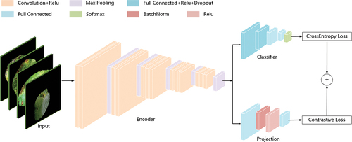
In this paper, we add projection head and contrastive loss function on the basis of Vgg16, and propose a supervised end-to-end contrastive learning-based deep convolutional neural network named CLCNN. CLCNN has three modules, encoder, classifier and projection head. The network structure of each module is shown in Figure 1. The data after data enhancement is input into the encoder, and the general image features of potato diseased leaves are extracted. The classifier is used to further abstract the high-level characteristics of potato diseases and classify the diseases of potato in different periods. Using the concept of contrastive learning, the projection head and contrastive loss functions are employed to further limit the representation learned by the encoder. As a result, fine-grained potato disease identification accuracy has improved.

Figure 1. CLCNN’s model architecture.

Data Source

Potato Research Institute of Yunnan Normal University is the first potato research institute in China. Combined with the excellent potato planting conditions and industrial support in Yunnan Province, great achievements have been made in potato research. The images of potato diseased leaves used in this paper are collected from Internet and the potato plantation of the Potato Research Institute of Yunnan Normal University, a total of 169. They are all taken by different people with mobile phones in the natural environment. The requirements for shooting technology and equipment are not high. The shooting distance, angle, lighting conditions, and camera equipment are not the same. They have different complex backgrounds and are very close to the actual application environment. The training set and the test set are divided in a ratio of 6 : 2. In this paper, two diseases of potato early blight and late blight were selected. The degree of potato early blight and late blight was subdivided into 8 categories, and each degree was clearly defined, see Table 1 and Figure 2. Early_1 to Early_4 represent the initial, early, middle and late stages of potato early blight. Late_1 to Late_4 represent the initial, early, middle and late stages of potato late blight.

Figure 2. Examples of potato early blight and late blight in each period.

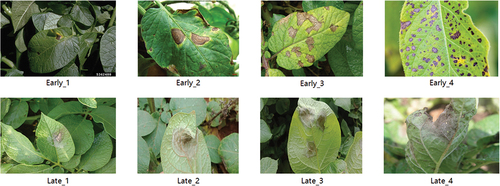
Table 1. Definition of disease period of potato early blight and late blight.

	Early_1	Early_2	Early_3	Early_4	Late_1	Late_2	Late_3	Late_4
number of lesions	0-3	4-10	10-20	>20	1	1-2	3-5	>5
total lesion area	<5%	5%-15%	15%-30%	>30%	<5%	5%-10%	10%-20%	>20%

Data Augmentation

Data augmentation is necessary to improve the results of small data sets. The data of potato disease images were augmented by left and right flip, up and down flip, contrast transformation, Gaussian noise (Camuto et al. 2020), brightness transformation, Gaussian noise plus brightness transformation. Compared with the original images, a total of 7 times of positive and negative samples were obtained, allowing contrastive learning to learn additional data consistency features. Data augmentation process is defined in Equation 1(1) $X=\{x_1,\dots ,x_i,\dots ,x_n\}$(1) , Equation 2(2) $\{a_{7i-6},\dots ,a_{7i}\}=\mathrm{\Gamma }(x_i)$(2) and Equation 3(3) $A=\mathrm{\Gamma }(X)=\{a_1,\dots ,a_i,\dots ,a_{7n}\}$(3) .

Assume that the input data has the following sample space:

(1) $X=\{x_1,\dots ,x_i,\dots ,x_n\}$(1)

$\mathrm{\Gamma }$ denotes data augmentation method, each of the samples is augmented into:

(2) $\{a_{7i-6},\dots ,a_{7i}\}=\mathrm{\Gamma }(x_i)$(2)

The enhanced sample space becomes:

(3) $A=\mathrm{\Gamma }(X)=\{a_1,\dots ,a_i,\dots ,a_{7n}\}$(3)

Network Structure

Encoder

Convolutional layers (Gu et al. 2018), ReLU activation functions (Agarap 2018), and max pooling layers (Brutzkus and Globerson 2021) are the primary components of the encoder. The receptive field and weight sharing methods employed by CNN reduce the amount of network training parameters, improve the optimization effectiveness of network parameters, and keep the picture well, which is why it was chosen as the encoder’s main backbone. CLCNN’s encoder is pre-trained with VGG16’s weights, and its purpose is to extract common features of potato disease leaves via transfer learning. Let $H_i$ represent the feature representation of the i-th encoder network layer, then $H_i$ can be generated as follows Equation 4(4) $H_i=(H_{i-1}{\kappa }_i)\upsilon {\nu }^{\ast }$(4) :

(4) $H_i=(H_{i-1}{\kappa }_i)\upsilon {\nu }^{\ast }$(4)

Where $H_{i-1}$ represents the feature of the previous network layer, ($H_0$ represents the original input), ${\kappa }_i$ represents the convolution kernel of the current convolutional layer, $\upsilon$ represents the ReLU function, $\nu$ represents the max pooling function, and ${ }^{\ast }$ represents quantity is not fixed, please refer to Figure 1 for the specific quantity. The feature $E$ encoded by the encoder is expressed as Equation 5(5) $E=Encoder(A)$(5) :

(5) $E=Encoder(A)$(5)

The network structure and input and output parameters of the encoder are shown in Table 2.

Table 2. Network structure of CLCNN’s encoder. $Vgg{16}^{\ast }$ represents the feature extractor and max pooling layer of Vgg16. Please refer to (Simonyan and Zisserman 2014) for the specific network structure of Vgg16.

Module	Network	Input size	Output size
Encoder	$Vgg{16}^{\ast }$	650*65	25088

Classifier

To lower the dimension of the characteristics learned by the encoder and gradually abstract the high level aspects of potato illness photos, the classifier employs four layers of fully connected neural networks (Ding et al. 2021), two ReLU functions, one Dropout function (Liang et al. 2021), and one Softmax function (Niklaus and Liu 2020). The relationship of present network layer feature $S_i$ and the preceding network layer feature relationship $S_{i-1}$ is written as Equation 6(6) $S_i=(S_{i-1}{W_i}^{\prime }+{B_i}^{\prime }){\upsilon }^{\ast }{\delta }^{\ast }{\xi }^{\ast }$(6) :

(6) $S_i=(S_{i-1}{W_i}^{\prime }+{B_i}^{\prime }){\upsilon }^{\ast }{\delta }^{\ast }{\xi }^{\ast }$(6)

Where $S_0$ denotes the input of Classifier. $W_i$ is the weight of the fully connected neural network in the i-th layer. $B_i$ is the offset vector of the fully connected neural network in the i-th layer. $\upsilon$ is the ReLU function. $\delta$ is the Dropout function. $\xi$ is the Softmax function, and ${ }^{\ast }$ represents quantity is not fixed, please refer to Figure 1 for the specific quantity.

The diseased image features extracted by the encoder code are passed through the classifier, and finally a 1-dimensional vector ($Y$) of size 8 is obtained as Equation 7(7) $Y=Classifier(E)$(7) :

(7) $Y=Classifier(E)$(7)

Where $Y$ represents the probability of each disease period identified by the model, and the largest probability is the degree of potato disease predicted by CLCNN.

The network structure and input and output parameters of the classifier are shown in Table 3.

Table 3. Network structure of CLCNN’s classifier. Vgg16** represents the classifier of Vgg16 that lacks the last fully connected layer. Please refer to (Simonyan and Zisserman 2014) for the specific network structure of Vgg16.

Module	Network	Input size	Output size
Classifier	$Vgg{16}^{\ast \ast }$	25088	1000
	Fully connected layer	1000	8
	Softmax	8	8

Projection Head

The function of the projection head is to further filter the features extracted by the encoder to extract more features related to the contrastive learning task. The reason for this is that the encoder using transfer learning extracts the general features of the diseased image, which contains many task independent features. The projection head consists of 2 layers of fully connected neural network, 1 BatchNorm function (Sari, Belbahri, and Partovi Nia 2019), and 1 ReLU function. The two layer fully connected neural network reduces the 1-dimensional vector feature of size 25,088 output by the encoder to a 1-dimensional vector feature of size 128. It will be used as input to the contrastive learning loss function, expressed as Equation 8(8) $\begin{array}{cc}Z& =Projection(E)\\ \hspace{0.17em}& =(E{W_1}^{\prime \prime }+{B_1}^{\prime \prime })\delta \upsilon (E{W_2}^{\prime \prime }+{B_2}^{\prime \prime })\end{array}$(8) :

(8) $\begin{array}{cc}Z& =Projection(E)\\ \hspace{0.17em}& =(E{W_1}^{\prime \prime }+{B_1}^{\prime \prime })\delta \upsilon (E{W_2}^{\prime \prime }+{B_2}^{\prime \prime })\end{array}$(8)

Where $W_1$ and $W_2$ represent the weights of the two layer fully connected neural network. $B_1$ and $B_2$ represent the offset vector. $\delta$ represents the BatchNorm function, and $\upsilon$ represents the ReLU function.

The network structure and input and output parameters of the projection head are shown in Table 4.

Table 4. Network structure of CLCNN’s projection head.

Module	Network	Input size	Output size
Projection head	Fully connected layer	25088	512
	BatchNorm	512	512
	ReLU	512	512
	Fully connected layer	512	128

Contrastive Representation Learning

Construction of Positive and Negative Examples

Because positive and negative examples are the objects of contrastive learning, the selection and construction of positive and negative examples is crucial. As previously stated, our goal is to identify fine-grained potato disease and research methodologies that are suitable for a small number of datasets and can improve classification accuracy over time. According to the dataset’s label, we utilize data with the same category label as a positive example and data with a different category label as a negative example. Specifically, in the same training batch, the category data with the largest number of labels is selected as the positive example, and the data of other categories is used as the negative example relative to the positive example. The positive sample set $P$ and the negative sample set $N$ are then expressed as Equation 9(9) $P=\{z_i|f(z_i)=g(Z)\}$(9) and Equation 10(10) $N=\{z_i|f(z_i)\ne g(Z)\}$(10) :

(9) $P=\{z_i|f(z_i)=g(Z)\}$(9)

(10) $N=\{z_i|f(z_i)\ne g(Z)\}$(10)

Where the function $f(z_i)$ represents the category of data obtained according to the existing label in the projection head’s output space $Z$, while the function $g(Z)$ represents the category with the largest number in the space $Z$.

Contrastive Loss Function

The loss function is separated into two parts: the classification loss function, which employs the cross entropy loss function, and the comparative learning loss function. The final joint loss function is obtained by adding the values of the two loss functions. The following section focuses on contrastive learning’s loss function.

Use the quantity product to calculate the similarity between two feature vectors. The overall similarity of positive examples is equal to the sum of the pairwise products of all elements in the positive example set $P$, denoted as $\alpha$. The overall similarity of negative examples is equal to the sum of the pairwise products of all elements in the negative example set $N$, denoted as $\beta$. $\alpha$ and $\beta$ are expressed as follows Equation 11(11) $\alpha =\sum _{i\ne j}^{p\in P}{p}_i\cdot p_j$(11) and Equation 12(12) $\beta =\sum _{i\ne j}^{n\in N}{n}_i\cdot n_j$(12) :

(11) $\alpha =\sum _{i\ne j}^{p\in P}{p}_i\cdot p_j$(11)

(12) $\beta =\sum _{i\ne j}^{n\in N}{n}_i\cdot n_j$(12)

Because the BatchNorm function is used for normalization in the projection head, the result of the quantity product is proportional to the cosine of the angle between the feature vectors. Therefore, the quantity product can be used to measure the similarity between two feature vectors.

The goal of contrastive learning is to make the similarity between positive example features larger and the similarity between negative example features smaller. Therefore, when studying the loss function of contrastive learning, we chose the negative logarithmic function. In order to eliminate the influence of the logarithmic function on the similarity, the natural base is used as the base of the similarity. In addition, a hyperparameter $\tau$ is added to adjust the difference in the similarity of positive and negative examples, thereby adjusting the distance range between positive and negative examples in the latent space. The smaller the $\tau$, the larger the distance between positive and negative examples, and the less training is required. The larger the $\tau$, the smaller the distance between positive and negative examples, and the more training is required. The choice of $\tau$ is not as small as possible, because the number of training times requires balancing the classifier and projection head to make the features they learn as good as possible. The loss function formula for contrastive learning is as follows Equation 13(13) ${\mathrm{\ell }}_c=-log\frac{\mathrm{e}\mathrm{x}\mathrm{p}(\alpha /\tau )}{\mathrm{e}\mathrm{x}\mathrm{p}(\alpha /\tau )+\mathrm{e}\mathrm{x}\mathrm{p}(\beta /\tau )}$(13) :

(13) ${\mathrm{\ell }}_c=-log\frac{\mathrm{e}\mathrm{x}\mathrm{p}(\alpha /\tau )}{\mathrm{e}\mathrm{x}\mathrm{p}(\alpha /\tau )+\mathrm{e}\mathrm{x}\mathrm{p}(\beta /\tau )}$(13)

Table

Algorithm 1:CLCNN’s main learning algorithm.
Input: Potato disease images $X$, batch size $n$, structure of $\mathbb{E}$,$\mathbb{C}$,$\mathbb{P}$, function of $\mathrm{\Gamma }$,$f$,$g$, constant $\tau$
1 for sampled minibatch $\{x_i{\}}_{i=1}^n$ do
2 for $i\in \{1,\dots ,n\}$ do
3 $\{a_{7i-6},\dots ,a_{7i}\}=\mathrm{\Gamma }(x_i)$	# Data augmentation
4 define $P=\{\}$	# Positive examples
5 define $N=\{\}$	# Negative examples
6 for $j\in \{1,\dots ,7n\}$ do
7 $e_j=\mathbb{E}(a_j)$	# Encoder
8 $y_j=\mathbb{C}(e_j)$	# Classifier
9 $z_j=\mathbb{P}(e_j)$	# Projection head
10 # get category function $f$
11 # get most category function $g$
12 if $f(z_i)=g(Z)$ then
13 push $z_i$ to $P$
14 else
15 push $z_i$ to $N$
16 define $\alpha =0$# Positive examples’ similarity
17 define $\beta =0$# Negative examples’ similarity
18 for $k\in \{1,\dots ,7n\}$ do
19 for $m\in \{1,\dots ,7n\}$ do
20 if $z_k\in P$ and $z_m\in P$ and $z_k\ne z_m$ then
21 $\alpha =\alpha +z_k\cdot z_m$	# Update $\alpha$
22 if $z_k\in N$ and $z_m\in N$ and $z_k\ne z_m$ then
23 $\beta =\beta +z_k\cdot z_m$	# Update $\beta$
24 # CrossEntropy loss
25 define ${\mathrm{\ell }}_{ce}={\sum }_{j\in 7n}lable(y_j)log(y_j)$
26 # Contrastive loss
27 define ${\mathrm{\ell }}_c=-log\frac{\mathrm{e}\mathrm{x}\mathrm{p}(\alpha /\tau )}{\mathrm{e}\mathrm{x}\mathrm{p}(\alpha /\tau )+\mathrm{e}\mathrm{x}\mathrm{p}(\beta /\tau )}$
28 # Joint loss
29 define $\mathcal{L}={\mathrm{\ell }}_{ce}+{\mathrm{\ell }}_c$
30 Update networks’ parameters to minimize $\mathcal{L}$
Output:Predicted potato diseases $Y$

The above formula is deformed to obtain: ${\mathrm{\ell }}_c=-log(1+exp(\beta /\tau )/exp(\alpha /\tau ))$. It is not difficult to find that ${\mathrm{\ell }}_c$ decreases as $\alpha$ increases and $\beta$ decreases. Therefore, the contrastive loss function implements the idea of contrastive learning, that is, increasing the similarity between positive examples and reducing the similarity between negative examples.

Finally, the loss function value ${\mathrm{\ell }}_c$ of the contrastive learning and the cross entropy loss function value ${\mathrm{\ell }}_{ce}$ of the classification are added to obtain the joint loss function value $\mathcal{L}$, as described in Equation 14(14) $\mathcal{L}={\mathrm{\ell }}_{ce}+{\mathrm{\ell }}_c$(14) . The joint loss function is used to update all weight parameters of the entire CLCNN model, thus forming a supervised end-to-end contrastive learning-based convolutional neural network model.

(14) $\mathcal{L}={\mathrm{\ell }}_{ce}+{\mathrm{\ell }}_c$(14)

Algorithm 1 summarizes the proposed method.

Experiments

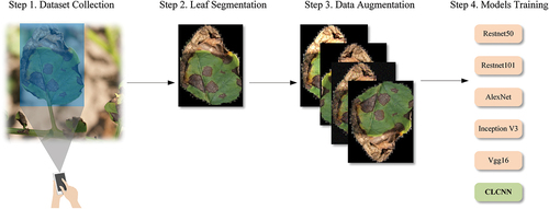
To verify the feasibility of the proposed CLCNN model, we designed and completed experiments for fine-grained potato disease identification. The experimental process is divided into the following steps. First, the leaf images of potato early blight and late blight in different disease periods are collected, and then the Mask-RCNN (Kaiming et al. 2017) model is used to segment the diseased leaf images. The rest of the background is set to black, and then 6 data enhancement methods is used to expand the dataset, and finally the expanded dataset is input into the CLCNN model for training and testing, as shown in Figure 3. To verify the performance improvement of the CLCNN model, we also compare it with Resnet50 (Kaiming et al. 2016), Resnet101 (Zhang 2022), AlexNet (Krizhevsky et al. 2012), Inception V3 (Szegedy et al. 2016), Vgg16 (Simonyan and Zisserman 2014). Finally, the experimental results of the CLCNN model are analyzed and summarized.

Figure 3. Process of CLCNN’s experiments.

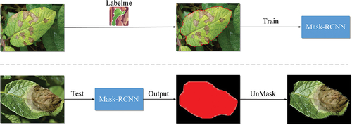
Leaf Segmentation

Because the potato disease pictures are taken in the natural environment, affected by the light and soil environment, the background is complex, which has a great influence on the identification accuracy of potato diseases. Therefore, it is necessary to remove the complex background of the image and segment the diseased leaves.

This paper uses Mask R-CNN to segment diseased potato leaves. Mask R-CNN is a general instance segmentation framework, which is a branch of Fast R-CNN (Meng et al. 2018). In order to use the Mask R-CNN model, we first need to label the diseased potato leaves using the Labelme (Lu, Yifan, and Xiao 2019) tool. These labeled data are then used to train a Mask RCNN model, and the trained model is used to segment images of potato leaves with complex backgrounds in natural environments. The experimental process of plant disease leaf segmentation is shown in Figure 4.

Figure 4. The experimental process of using Mask-RCNN to segment plant diseased leaves.

Data Augmentation

Due to time and human resource cost constraints, there are few data on potato disease in natural contexts, so it is crucial to use data-augmented methods to make it more effective. Data augmentation means making a limited amount of data yield value equivalent to more data without adding more data (Shorten and Khoshgoftaar 2019), while also increasing the number of positive and negative examples for contrastive learning, making the effect of contrastive learning better. This paper uses python’s skimage library to perform six image transformations on each segmented plant disease image, including left and right flip, up and down flip, contrast transformation, Gaussian noise, brightness transformation, Gaussian noise plus brightness transformation, as shown in Figure 5. The augmented dataset has a total of 1183 images, and the number of images in each period is shown in Table 5.

Figure 5. Six methods of data augmentation.

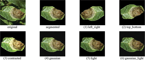
Table 5. Results of data augmentation.

	Early_1	Early_2	Early_3	Early_4	Late_1	Late_2	Late_3	Late_4	total
original	10	10	28	25	6	25	32	33	169
augmentated	70	70	196	175	42	175	224	231	1183

Model Training

The matrix calculation of deep learning needs enough GPU computing power to support. The GPU we use is NVIDIA Tesla T4 16GB, the server environment is Windows 10 64-bit operating system, and the CPU is Intel(R) Xeon(R) Gold 5117 CPU @ 2.00 GHz 2.00 GHz. The deep learning framework of choice is Pytorch, and based on this framework, we built the experimental data reading, model definition, training, and testing code from scratch. Under the above hardware and software conditions, the training time of our CLCNN model is about 12 hours. In addition to training the CLCNN model, we also trained Resnet50, Resnet101, AlexNet, Vgg16, Inception V3 models for comparison. The hyperparameter settings of the model are shown in Table 6. The source code of the paper is https://github.com/woldcn/CLCNNhttps://github.com/woldcn/CLCNN.

Table 6. Hyperparameters of CLCNN. $\tau$ refers to Equation 13(13) ${\mathrm{\ell }}_c=-log\frac{\mathrm{e}\mathrm{x}\mathrm{p}(\alpha /\tau )}{\mathrm{e}\mathrm{x}\mathrm{p}(\alpha /\tau )+\mathrm{e}\mathrm{x}\mathrm{p}(\beta /\tau )}$(13) .

model	hyperparameters	value
CLCNN	learn_rate	1e-05
	$\tau$	0.8
	batch_size	10
	epochs	200
	rand_seed	42

Results and Discussions

In the experiment of fine-grained potato disease recognition, we compared the proposed CLCNN model with five other models which have good effects in the field of image recognition. We recorded the change of accuracy during the training and testing of each model, as shown in Figure 7. It is not difficult to find that the accuracy curve of CLCNN model is more stable and the upward trend is more obvious. It shows that the model has better denoising ability and learning ability by filtering and further restricting the general features of diseases by contrastive learning pro-jection head. It is proved that the proposed CLCNN model is suitable for fine-grained potato disease identification.

After 200 training iterations, we recorded the highest accuracy of the 6 models on the test set, as shown in Table 7. The confusion matrix of classification results is presented in Figure 6. Among them, the accuracy of our proposed CLCNN model is 97.24%, higher than 90.28% of Resnet50, 90.62% of Resnet101, 93.06% of AlexNet, 94.44% of Inception V3, and 94.79% of Vgg16. It was 6.96% higher than Resnet50 and 2.45% higher than Vgg16. This shows that our proposed method is feasible and superior to the other five main image recognition models.

Figure 6. Confusion matrix of the classification results.

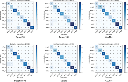
Figure 7. Accuracy curves for training and testing of each model.

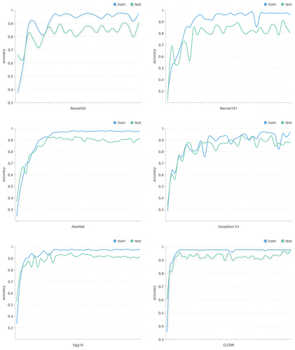
Table 7. The highest accuracy of the 6 models on test set.

Models	Resnet50	Resnet101	AlexNet	Inception V3	Vgg16	CLCNN
accuracy	90.27	90.62	93.05	94.44	94.79	97.24

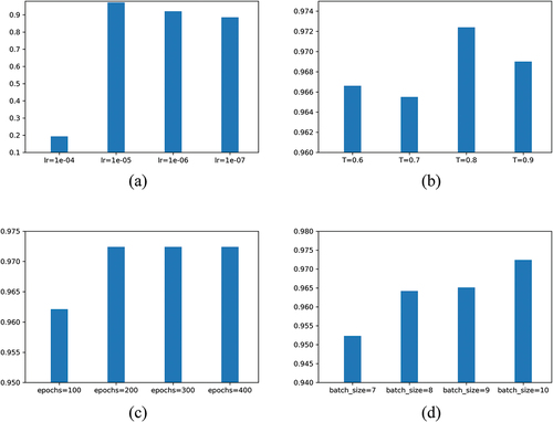
We tried multiple hyperparameters tuning using the fixed variable method, and the best results for each parameter on the test set are shown in Figure 8. It can be seen from Figure 8 (a) and (b) that there is an optimal value for the learning rate and temperature hyperparameters. Below or above this value, the accuracy will decrease. Moreover, the learning rate cannot be set too high, and the model cannot be fitted after being higher than 1e-05. After the number of iterations exceeds 200, the accuracy of the model no longer rises, indicating that the model and data do not require too many iterations and can converge quickly within a limited number of iterations, as shown in Figure 8 (c). Limited by GPU (Tesla T4) hardware conditions, we experimented with batch sizes up to 10 pictures. Figure 8 (d) shows that as the batch size increases, the accuracy of the model increases. We analyzed the reason that each batch needs to have enough samples to support positive and negative sampling. The larger the batch, the richer the sampling of positive and negative samples, and the more valuable the contrast loss calculated by Equation 13(13) ${\mathrm{\ell }}_c=-log\frac{\mathrm{e}\mathrm{x}\mathrm{p}(\alpha /\tau )}{\mathrm{e}\mathrm{x}\mathrm{p}(\alpha /\tau )+\mathrm{e}\mathrm{x}\mathrm{p}(\beta /\tau )}$(13) . At the same time, this is also a limitation of the model, which requires certain hardware conditions to support a sufficient size of batch data. If the memory is not enough, it will cause overflow errors. Whether the larger the batch, the better, which requires us to have better hardware conditions later experimental verification.

Figure 8. The highest accuracy of CLCNN on different hyperparameters. lr denotes learn_rate. $\tau$ refers to Equation 13(13) ${\mathrm{\ell }}_c=-log\frac{\mathrm{e}\mathrm{x}\mathrm{p}(\alpha /\tau )}{\mathrm{e}\mathrm{x}\mathrm{p}(\alpha /\tau )+\mathrm{e}\mathrm{x}\mathrm{p}(\beta /\tau )}$(13) .

In order to deeply analyze the reason why the proposed CLCNN model has higher accuracy, we remove the projection head and contrast loss function in the CLCNN model, and the remaining model network is basically consistent with the network module of Vgg16. The encoder still uses the pre-training weights of Vgg16. We evaluated the recognition accuracy, recall rate, specificity and F1 score of the two models in different degrees of potato early blight and late blight,, as shown in Table 8. The results show that the CLCNN model has improved significantly in five of them. It shows that the CLCNN model using the idea of contrastive learning not only obtains higher accuracy, but also more comprehensive identification and lower probability of error in fine-grained potato disease identification. It is proved that the supervised contrastive convolution neural network is effective.

Table 8. Precision, recall, specificity, and F1 score of Vgg16 and CLCNN in each period.

Vgg16	Early_1	Early_2	Early_3	Early_4	Late_1	Late_2	Late_3	Late_4
precision	1.0	1.0	0.961	1.0	0.933	0.93	0.902	0.942
recall	0.667	1.0	1.0	0.886	1.0	0.952	0.982	0.98
specificity	1.0	1.0	0.992	1.0	0.996	0.988	0.974	0.987
F1 score	0.8	1.0	0.98	0.9394	0.965	0.9412	0.9402	0.9608
CLCNN	Early_1	Early_2	Early_3	Early_4	Late_1	Late_2	Late_3	Late_4
precision	1.0	0.84	1.0	1.0	0.933	1.0	0.949	1.0
recall	0.667	1.0	1.0	1.0	1.0	0.976	1.0	1.0
specificity	1.0	0.985	1.0	1.0	0.996	1.0	0.987	1.0
F1 score	0.8	0.913	1.0	1.0	0.965	0.988	0.973	1.0

Conclusions

Deep learning is an effective method for plant disease identification. In order to make the characteristics of potato in different disease stages more dispersed in the latent space, so as to improve the classification accuracy, we studied the contrastive learning which has been developed in the past two years. In this study, we proposed a deep convolutional neural network (CLCNN) based on supervised end-to-end contrastive learning for the identification of fine-grained potato diseases. Through many comparative experiments, the main conclusions of the model are as follows : (1) The CLCNN model improves the similarity between similar sample features and reduces the similarity between different sample features, and makes the samples of different classes have better discrimination. (2) CLCNN model can effectively improve the accuracy of fine-grained potato disease identification. (3) The previous contrastive learning methods extract features in the pre-training stage, and the contrastive learning of CLCNN is directly used for classification tasks, indicating that the contrastive learning method can also achieve good results when directly applied to downstream tasks. In fact, the projection head module based on contrastive learning in the CLCNN model can be integrated into all supervised classification models, which is expected to improve the accuracy of all classification tasks. In the following work, we will try more research and experiments to prove this.

Acknowledgments

This work is supported by the National Natural Science Foundation of China (No. 61862067); Applied Basic Research Project in Yunnan Province (No.202101AT070132); Prevention and control of potato wilt disease, YNNU-YINMORE Cooperative Project (No.021110301).

Disclosure statement

No potential conflict of interest was reported by the author(s).

Additional information

Funding

This work was supported by the Engineering Research Center of Sustainable Development and Utilization of Biomass Energy, Ministry of Education; Key Lab of Yunnan Province for Biomass Energy and Environmental Biotechnology.

References

- Agarap, A. F. 2018. Deep learning using rectified linear units (relu). arXiv preprint arXiv:180308375. doi:10.48550/arXiv.1803.08375.
- Andreas, K., and F. X. Prenafeta-Boldĺš. 2018. Deep learning in agriculture: A survey. Computers and Electronics in Agriculture 147:70–314. doi:10.1016/j.compag.2018.02.016.
- Brutzkus, A., and A. Globerson. 2021. An optimization and generalization analysis for max-pooling networks. Uncertainty in Artificial Intelligence, Online, 1650–60. PMLR.
- Camuto, A., M. Willetts, U. Simsekli, S. J. Roberts, and C. C. Holmes. 2020. Explicit regularisation in gaussian noise injections. Advances in Neural Information Processing Systems 33:16603–14.
- Chen, X., and H. Kaiming 2021. Exploring simple siamese representation learning. In Proceedings of the IEEE/CVF Conference on Computer Vision and Pattern Recognition, 15750–58. doi:10.48550/arXiv.2011.10566.
- Chen, T., S. Kornblith, M. Norouzi, and G. Hinton. 2020. A simple framework for contrastive learning of visual representations. In International conference on machine learning, Virtual, 1597–607. PMLR.
- Chen, J., Q. Liu, and L. Gao. 2019. Visual tea leaf disease recognition using a convolutional neural network model. Symmetry 11 (3):343. doi:10.3390/sym11030343.
- Devlin, J., M.W. Chang, K. Lee, and K. Toutanova. 2018. Bert: Pre-training of deep bidirectional transformers for language understanding. arXiv preprint arXiv:181004805. doi:10.48550/arXiv.1810.04805.
- Ding, X., C. Xia, X. Zhang, X. Chu, J. Han, and G. Ding. 2021. Repmlp: Re-parameterizing convolutions into fully-connected layers for image recognition. arXiv preprint arXiv:210501883. doi:10.48550/arXiv.2105.01883.
- Dongyu, Q. 2022. Doubling global potato production in 10 years is possible. https://www.fao.org.
- Geng, Z., Q. Meng, J. Bai, J. Chen, Y. Han, Q. Wei, and Z. Ouyang. 2019. A model-free bayesian classifier. Information Sciences 482:171–88. doi:10.1016/j.ins.2019.01.026.
- Goodfellow, I., J. Pouget-Abadie, M. Mirza, X. Bing, D. Warde-Farley, S. Ozair, A. Courville, and Y. Bengio. 2014. Generative adversarial nets. Advances in Neural Information Processing Systems 27. doi:10.1145/3422622.
- Grill, J. B., F. Strub, F. Altché, C. Tallec, P. Richemond, E. Buchatskaya, C. Doersch, B. A. Pires, Z. Guo, M. G. Azar, et al. 2020. Bootstrap your own latent-a new approach to self-supervised learning. Advances in Neural Information Processing Systems 33:21271–84.
- Gu, J., Z. Wang, J. Kuen, L. Ma, A. Shahroudy, B. Shuai, T. Liu, X. Wang, G. Wang, J. Cai, et al. 2018. Recent advances in convolutional neural networks. Pattern recognition 77:354–77. doi:10.1016/j.patcog.2017.10.013.
- Hao, P.Y., J.H. Chiang, and Y.D. Chen. 2022. Possibilistic classification by support vector networks. Neural Networks 149:40–56. doi:10.1016/j.neunet.2022.02.007.
- Hossain, S., R. Mumtahana Mou, M. Mahedi Hasan, S. Chakraborty, and M. Abdur Razzak. 2018. Recognition and detection of tea leaf’s diseases using support vector machine. In 2018 IEEE 14th International Colloquium on Signal Processing & Its Applications (CSPA), 150–54. IEEE. doi:10.1109/CSPA.2018.8368703.
- Junde, C., J. Chen, D. Zhang, Y. Sun, and Y. A. Nanehkaran. 2020. Using deep transfer learning for image-based plant disease identification. Computers and Electronics in Agriculture 173:105393. doi:10.1016/j.compag.2020.105393.
- Kaiming, H., H. Fan, W. Yuxin, S. Xie, and R. Girshick. 2020. Momentum contrast for unsupervised visual representation learning. In Proceedings of the IEEE/CVF conference on computer vision and pattern recognition, 9729–38. doi:10.48550/arXiv.1911.05722.
- Kaiming, H., G. Gkioxari, P. Dollár, and R. Girshick. 2017. Mask r-cnn. In Proceedings of the IEEE international conference on computer vision, 2961–69. doi:10.48550/arXiv.1703.06870.
- Kaiming, H., X. Zhang, S. Ren, and J. Sun. 2016. Deep residual learning for image recognition. In Proceedings of the IEEE conference on computer vision and pattern recognition, Las Vegas, 770–78.
- Khosla, P., P. Teterwak, C. Wang, A. Sarna, Y. Tian, P. Isola, A. Maschinot, C. Liu, and D. Krishnan. 2020. Supervised contrastive learning. Advances in Neural Information Processing Systems 33:18661–73.
- Kiani, E., and T. Mamedov. 2017. Identification of plant disease infection using soft-computing: Application to modern botany. Procedia computer science 120:893–900. doi:10.1016/j.procs.2017.11.323.
- Krizhevsky, A., I. Sutskever, G. E. Hinton, and E. P. Simoncelli. 2012. Efficient and direct estimation of a neural subunit model for sensory coding. Advances in Neural Information Processing Systems 25:3113–21. doi:10.1145/3065386.
- Liang, X., L. Wu, J. Li, Y. Wang, Q. Meng, T. Qin, W. Chen, M. Zhang, T. Y. Liu. 2021. R-drop: Regularized dropout for neural networks. Advances in Neural Information Processing Systems 34:10890–905.
- Li, K., J. Lin, J. Liu, and Y. Zhao. 2020. Using deep learning for image-based different degrees of ginkgo leaf disease classification. Information 11 (2):95. doi:10.3390/info11020095.
- Lu, Y., H. Yifan, and J. Xiao. 2019. Help LabelMe: A fast auxiliary method for labeling image and using it in ChangE’s CCD data. In International Conference on Image and Graphics, 801–10. Springer. doi:10.1007/978-3-030-34120-665.
- Meng, R., S. G. Rice, J. Wang, and X. Sun. 2018. A fusion steganographic algorithm based on faster R-CNN. Computers, Materials & Continua 55 (1):1–16. doi:10.3970/cmc.2018.055.001.
- Nasr-Esfahani, M. 2022. An IPM plan for early blight disease of potato alternaria solani sorauer and A. alternata (fries.) Keissler. Archives of Phytopathology and Plant Protection 55 (7):785–96. doi:10.1080/03235408.2018.1489600.
- Nazki, H., S. Yoon, A. Fuentes, and D. Sun Park. 2020. Unsupervised image translation using adversarial networks for improved plant disease recognition. Computers and Electronics in Agriculture 168:105117. doi:10.1016/j.compag.2019.105117.
- Niklaus, S., and F. Liu. 2020. Softmax splatting for video frame interpolation. In Proceedings of the IEEE/CVF Conference on Computer Vision and Pattern Recognition, Virtual, 5437–46.
- Ning, Y., Y. Qian, H. S. EL-Mesery, R. Zhang, A. Wang, and J. Tang. 2019. Rapid detection of rice disease using microscopy image identification based on the synergistic judgment of texture and shape features and decision tree–confusion matrix method. Journal of the Science of Food and Agriculture 99 (14):6589–600. doi:10.1002/jsfa.9943.
- Sari, E., M. Belbahri, and V. Partovi Nia. 2019. How does batch normalization help binary training? arXiv preprint arXiv:190909139 arXiv preprint arXiv:190909139. doi:10.48550/arXiv.1909.09139.
- Sharma, S., and M. Lal. 2022. Advances in Management of Late Blight of Potato 163–84. Springer. 10.1007/978-981-16-7695-67
- Shorten, C., and T. M. Khoshgoftaar. 2019. A survey on image data augmentation for deep learning. Journal of Big Data 6 (1):1–48. doi:10.1186/s40537-019-0197-0.
- Simonyan, K., and A. Zisserman. 2014. Very deep convolutional networks for large-scale image recognition. arXiv preprint arXiv:14091556. doi:10.48550/arXiv.1409.1556.
- Sinaga, K. P., and M.S. Yang. 2020. Unsupervised K-means clustering algorithm. IEEE Access 8:80716–27. doi:10.1109/ACCESS.2020.2988796.
- Szegedy, C., V. Vanhoucke, S. Ioffe, J. Shlens, and Z. Wojna. 2016. Rethinking the inception architecture for computer vision. In Proceedings of the IEEE conference on computer vision and pattern recognition, Las Vegas, 2818–26.
- Yang, L., Y. Shujuan, N. Zeng, Y. Liu, and Y. Zhang. 2017. Identification of rice diseases using deep convolutional neural networks. Neurocomputing 267:378–84. doi:10.1016/j.neucom.2017.06.023.
- Yan, Y., L. Rumei, S. Wang, F. Zhang, W. Wei, and X. Weiran. 2021. Consert: A contrastive framework for self-supervised sentence representation transfer. arXiv preprint arXiv:210511741. doi:10.48550/arXiv.2105.11741.
- Yuen, J. 2021. Pathogens which threaten food security: Phytophthora infestans, the potato late blight pathogen. Food Security 13 (2):247–53. doi:10.1007/s12571-021-01141-3.
- Zhang, Q. 2022. A novel ResNet101 model based on dense dilated convolution for image classification. SN Applied Sciences 4 (1):1–13. doi:10.1007/s42452-021-04897-7.