Spatial Simulation and Prediction of Air Temperature Based on CNN-LSTM

ABSTRACT

Predicting the air temperature based on spatially accurate simulations is helpful to agricultural production, commercial activities, air transportation, water transportation, power supply, and national defense. Traditional prediction is not generally based on the time series obtained from multiple meteorological stations and from a spatial perspective. In this study, a deep convolution neural network with long short-term memory (CNN-LSTM) is constructed to extract the spatiotemporal features of temperature and the correlation between meteorological elements. The accuracies of the simulated and the predicted temperatures are spatially visualized by using the Kriging interpolation method. The accuracy of air temperature obtained from the CNN-LSTM was compared with those obtained from the CNN and the LSTM to verify its performance. The results show that there were prominent spatial variations in the temperature, with a latitudinal zonal structure in the southern Ningxia and a radial zonal structure in the northern Ningxia, China. The accuracies of the simulated and predicted temperature were high in areas with a small range of the annual temperature. The accuracies of the mean monthly temperature simulated by the CNN-LSTM in spring and autumn were higher than that in the summer. The predicted annual average temperature increased each year from 2020 to 2025. The CNN-LSTM had a higher accuracy of simulating and predicting the temperature as well as a better generalization ability than the CNN and LSTM.

Introduction

The change in temperature is a dynamic and nonlinear process that is influenced by many factors, such as the solar radiation, the latitude, the positions of sea and land, atmospheric circulation, relative humidity, terrain, vegetation, air pressure, wind speed, and the ocean current (Abdel-Aal 2004; Ramesh and Anitha 2014). These factors are interrelated and interact with one another (Ye et al. 2013). The trend of changes in temperature in the future is difficult to fit by using a simple function because such changes have the characteristics of a temporal sequence, aggregation, asymmetry, spatiotemporal correlation, and conditional heteroscedasticity (Krasnopolsky and Fox-Rabinovitz 2006; Prior and Perry 2014). Integrating multivariate meteorological and spatial data, including the time series of temperature, can improve the accuracy of the simulated and predicted temperature (Murthy et al. 2021; Sebastian et al. 2018).

The methods used to predict temperature include numerical, statistical, spatial, machine learning-based, and deep learning-based models. Methods based on numerical prediction are mainly used to predict the temperature over a short-time series (Byeongseong et al. 2021; Stelian et al. 2019), but it is difficult to accurately simulate complex nonlinear atmospheric systems (Abramson et al. 1996). Statistical models, such as multiple regression, stepwise regression, autoregression, and moving average models, are generally used for predicting the temperature over a long time series according to probability density and cumulative distribution functions with statistical variables, such as latitude, altitude, aspect, slope, long-wave effective radiation, and total solar radiation (Asha, Santhosh, and Rishidas 2021; Livera, Hyndman, and Snyder 2011; Murat et al. 2016, 2018). Spatial models, such as the Kriging model, the inverse distance-weighted average model, and spline function, interpolate the temperature measured by discrete meteorological stations into a continuous temperature surface (Carrión et al. 2021; Liu et al. 2019; Xiao et al. 2019; Şahin 2012). Machine learning methods, such as the support vector machine, random forest, and artificial neural network (ANN), can be used to accurately predict the temperature over a short-time series (Astsatryan et al. 2021; Chevalier et al. 2011; Cifuentes et al. 2020; Gautier, Peterson, and Jones 1998; Gos et al. 2020; Hanoon et al. 2021; Hernández-Travieso et al. 2020; Lin, Tsai, and Chen 2021; Maqsood, Khan, and Abraham 2004; Mba, Meukam, and Kemajou 2016; Nury, Hasan, and Alam 2017; Ortiz-Garcia et al. 2012; Radhika and Shashi 2009; Tasadduq, Rehman, and Bubshait 2002; Tran et al. 2021; Ustaoglu, Cigizoglu, and Karaca 2008). In particular, ANN via optimization algorithms, such as genetic algorithm, can optimize its network structure and parameters (Abdolrasol et al. 2021).

Deep learning is the integration of neural network with graphical modeling, optimization, pattern recognition, and signal processing. Features of each layer in a deep learning model are extracted from the output of the previous layer for classification and prediction (Hou et al. 2022). Deep learning technology is being used commercially in many fields, such as mechanical fault diagnosis, text retrieval, energy prediction, stock market forecasting, image recognition, speech recognition, military target identification, process modeling and control, health diagnosis, portfolio management, magnetic resonance imaging, X-ray analysis, personal credit rating, marketing campaigns, unmanned driving, and financial fraud detection (Zhang, Dong, and Yuan 2020).

Deep learning has a strong ability for the processing of a large amount of nonlinear temperature data in a long time series to improve the accuracy of temperature prediction (Zhang et al. 2018). A variety of deep learning methods, such as the long short-term memory (LSTM), time-series diagram network, stacking automatic encoder, and convolution recurrent neural network, have been used to predict the temperature (Jeong et al. 2021). Bidirectional LSTM has outstanding robustness in predicting asphalt pavement temperature with an R² of 0.9555 compared with CNN, LSTM, and gated recurrent unit (Milad et al. 2021). The methods have good generalization, high accuracy, and fast convergence (Sekertekin et al. 2021). However, the methods are generally used to predict the temperature based on the time series obtained from a single meteorological station, instead of multiple meteorological stations. In addition, these methods are rarely used to simulate and predict the temperature from a spatial perspective (Yu, Shi, and Xu 2021).

The LSTM can map nonlinear changes in the time series of air temperature owing to its dynamic storage and memory (Mtibaa et al. 2020). The CNN can extract and compress feature vector to obtain the local spatial features of temperature (Sun et al. 2021). A combination of the LSTM and the CNN, a CNN-LSTM model, might be able to improve the accuracy of temperature prediction (Wang 2022). In this study, a CNN-LSTM model is constructed to simulate and predict the temperature obtained from meteorological stations in Ningxia, China, to verify its performance. The proposed model can capture the asymmetric dynamic and spatiotemporal characteristics of temperature. The spatial distributions of the measured and predicted temperatures are obtained by using the Kriging interpolation method. The accuracy of the temperature predicted by the CNN-LSTM was also compared with separate predictions by the LSTM and CNN to verify its performance. The novelty of this study is to build a CNN – LSTM model with a Kriging interpolation to spatiotemporally simulate and predict the hourly temperature time-series data collected from multiple meteorological stations with high accuracy. The work here provides guidance for decision-making on flood control, drought resistance, ecological protection, commercial activities, air transportation, water transportation, power supply, and national defense, and agricultural development.

Materials and Methods

Study Area and Data Processing

Ningxia is located in the middle and upper reaches of the Yellow River in northwestern China, between 35°14′ N and 39° 23′ N latitude and 104°17′ E and 107°39′ E longitude, with a total area of 6.64 × 104 km². The terrain tilts from the southwest to the northeast with altitudes ranging from 1077 m to 3512 m. The geomorphic types in the area include the Loess Plateau, the proluvial alluvial plain, Ordos platform, and the Liupan and Helan Mountains. The south, middle, and north of Ningxia are middle-temperature subhumid, semi-arid, and arid areas, respectively, with a dry climate, less rainfall, high winds and large amounts of sand, and large annual and daily ranges of temperature.

Meteorological data, such as meteorological station, time of data collection, hourly temperature, daily average, minimum, and maximum temperatures, rainfall, sunshine hours, wind speed, and air pressure, were collected from the National Meteorological Science Data Center of China. Repeated, abnormal, and discrete values in the collected dataset were preprocessed by filtering, filling, elimination, format conversion, and standardization.

The multicollinearity test and Pearson correlation analysis were used to calculate the variance expansion factor and correlation coefficient and screen the key meteorological elements affecting temperature prediction to eliminate redundant information. Key meteorological elements, such as the daily average, minimum, and maximum temperatures, rainfall, sunshine hours, and wind speed, were finally determined. Key meteorological data from January 2000 to December 2015 (180 months) were used as the training set, and data from January 2016 to December 2020 (60 months) were used as the validation set.

Construction of CNN-LSTM Model

The Tensorflow platform was used to construct the CNN-LSTM model. Tensorflow is an open-source software library for numerical calculations using deep neural networks. It supports the extended kernel library built on the CPU and the GPU, and is flexible.

The structure of CNN-LSTM is shown in Figure 1. In the model, the CNN is composed of an input layer, a convolution layer, a pooling layer, a full connection layer, and an output layer. The convolution layer is used to extract features of the data. The pooling layer is used for information screening and selection. The full connection layer is used to connect the CNN and the LSTM according to the softmax function. The output layer is used for feature classification. High-order features are extracted by the CNN, result in the decrease in the dimensionality of the input data x_t at time t, and outputs data h_t-1 at time (t − 1). x_t and h_t-1 are input into the LSTM. The hidden layer of the LSTM is composed of multiple memory units, each of which contains a forgetting gate, an input gate, and an output gate.

Figure 1. Structure of CNN-LSTM.

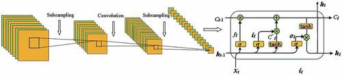
The forgetting gate is used to determine invalid information collected from the forgetting units. The inputs of the forgetting gate are the h_t-1 and x_t, and its output is the degree of forgetting f_t of the last cell in the cell state C_t-1 of the input at time (t − 1) after the calculation of the sigmoid function.

(1) $f_t=\left(W_f\left[h_{t-1},x_t\right]+b_f\right),$(1)

where f_t∈[0, 1] is the output of the forgetting gate, “0” means the information has been completely forgotten, “1” means that it has been completely retained, and W_f and b_f are the weight matrix and the bias term of the forgetting gate, respectively.

The input gate indicates the degree of update of the current information in a given cell state. The sigmoid function is used to update the value of i_t and tanh function is used to generate the state variable C_t.

(2) $i_t=\sigma \left(W_i\bullet \left[h_{t-1},x_t\right]+b_i\right),$(2)

(3) $C_t=tanh\left(W_C\bullet \left[h_t,x_t\right]+b_C\right),$(3)

where i_t is the output of the input gate, W_i and b_i are the weight matrix and bias term of the input gate, respectively, σ is the sigmoid activation function, C_t is the cell state of the current input, and W_c and b_c are the weight matrix and bias term of the cell state, respectively.

The output gate, which is the output layer after a cell state has been excited, is processed by the sigmoid and tanh functions to obtain the values [−1, 1] of the cell state.

(4) $o_t=\sigma \left(W_o\left[h_{t-1},x_t\right]+b_o\right),$(4)

(5) $h_t=o_t\bullet tanh\left(C_t\right),$(5)

where o_t is the output of the input gate, W_o and b_o are the weight matrix and bias term of the input gate, respectively, σ is the sigmoid activation function, and h_t is the output value.

The method of rolling prediction with one-step extrapolation is used to predict the temperature in the next five years. The meteorological data are divided into a subsample of estimation {x₁, x₂, ···, x_t-1 ,x_t} and a subsample of prediction {x_t+1 ,x_t+2, ···, x_t+i}. The dataset {x₁, x₂, ···, x_t-1 ,x_t} at time t is used to predict the temperature-related data {x₂, x₃, ···，x_t, x’_t+1 } at timet + 1, where x’_t+1 is the predicted value. The predicted value x’_t+1 is replaced by the measured value x_t+1 to predict x’_t+2 according to x_t+2.

Such observation data as daily average, minimum, and maximum temperatures, rainfall, sunshine hours, and wind speed, were obtained from 25 meteorological stations in Ningxia, China, were used to establish 25 predictive models of the CNN-LSTM. The annual average temperature recorded in each station was simulated from 2016 to 2020, and predicted from 2021 to 2025 to verify the generalization ability of the CNN-LSTM model.

The training and prediction processes of the CNN-LSTM model are as follows:

1. Initialize the network weight w and bias vector b, and set the window length and the maximum number of iterations.

2. Standardize the dataset to obtain x = {x₁, x₂, x₃, ···, x_n} with the interval [0, 1].

3. Divide x into a training set x_t = {x₁, x₂, x₃, ···, x_b} and a validation set x_v = {x_b + 1, x_b+2, x_b+3, ···, x_n}.

4. Obtain the predicted value x´_t from the training set x_t, and combined it with the last L − 1 elements after x_t to form a new training set. Input the new training set into the CNN-LSTM to obtain x´_t + 1, and so on, until the prediction set {x´_t, x´_t+1, ···, x´_n} has been constructed.

5. Inversely normalize the dataset {x´_t, x´_t+1, ···, x´_n} to obtain the predicted temperature {y_t, y_t+1, ···, y_n}.

6. Calculate the coefficient of determination R² to evaluate the performance of the CNN-LSTM model.

Spatial Interpolation

The air temperature can be spatially simulated and predicted according to the spatial relationship between adjacent meteorological stations. In this study, the Kriging method is used to interpolate the measured and the predicted temperatures as well as the predictive accuracy to obtain their spatial distributions. The potential relationship among meteorological stations in terms of air temperature is determined to reveal the spatial difference between the predicted and the measured temperatures.

Kriging interpolations, such as ordinary Kriging, simple Kriging, and collaborative Kriging, are methods of local spatial interpolation that form unbiased, optimal estimation of regionalized variables based on the assumption of stationary. Ordinary Kriging is used in this study as follows:

(6) $z_0=\sum _{i=1}^I{w}_i{z}_i.$(6)

where z₀ is the estimated value at point 0, w_i is the weight related to point i, z_i is the attribute value of point i, and i is the number of known points.

Results

Simulation of Air Temperature

A sensitivity analysis was conducted to investigate the relationships between the input and output variables of the CNN-LSTM model. There are many hyper-parameters of the CNN-LSTM model, such as input size, patch size, filter layer size, characteristic number, activation function, learning rate, and drop out.

Optuna is a software framework to automatically optimize super-parameters of a deep learning model based on historical data by trial and error. It could capture the interval of a parameter with high probability and discard that with low probability to improve search efficiency. Therefore, the optuna was selected in this study to analyze the sensitivity of the hyper-parameters to find the optimal combination of the hyper-parameters, in which the loss function value of the training data and the generalization error of the test set were both minimized. The optimal hyperparameters were obtained as follows: input size = 30, output size = 1, batch size = 128, number of epochs = 200, learning rate = 0.0001, and dropout = 0.5. The activation function was rectified linear unit (ReLU). The loss function is the mean absolute error (MAE). The Adam optimizer was applied.

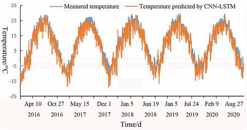
The prior knowledge is added to the CNN-LISTM model, including the original network structure, initial weight, layer-wise learning rate decay, constraints to the loss function, and freeze of the deep weight of the backbone. The prior distribution is the probability distribution of the current temperature. The posterior distribution of temperature is updated dynamically, which is the normalization of the product of prior distribution of the current temperature and likelihood function of the next measured temperature. Figure 2 shows the curves of the prior measured and posterior temperatures collected from the Yinchuan meteorological station, Ningxia, China, from 1 January 2016 to 31 December 2020 simulated by CNN – LSTM. The posterior temperatures simulated by the CNN – LSTM model coincided with the prior measured temperatures.

Figure 2. Prior measured and posterior temperatures from 2016 to 2020 simulated by CNN – LSTM.

The annual average temperature measured from 25 meteorological stations in Ningxia was interpolated by using the ordinary Kriging in ArcGIS 10.6 to compare the measured temperature with the simulated and predicted values. Figure 3a shows the characteristics of distribution of the annual average temperature measured in 2016. It was between 6.9°C and 11.5°C and was high in the north and low in the south. The annual average temperature in Yuanzhou District, Xiji County, Jingyuan County, and Longde County was lower than 9°C. However, the annual average temperature in Zhongning and Litong was higher than 11°C. The low temperature in southern Ningxia occurred owing to the high altitude of the Liupan Mountains. The high temperature in the northwestern Ningxia occurred because the Helan Mountains on the western border of Ningxia block the cold, westerly wind in winter from flowing into northwestern Ningxia.

Figure 3. The distribution of the annual average temperature in 2016, measured (a) and simulated by the CNN-LSTM (b).

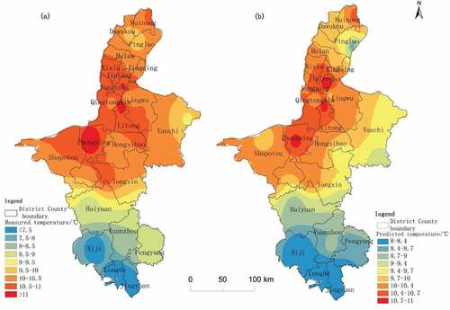
The eigenmatrix of the key meteorological elements in 2016 at each meteorological station was input to the CNN-LSTM model to obtain the simulated average temperature at the meteorological stations on the next day. The monthly and annual average temperatures of each meteorological station were calculated according to the simulated daily average temperature. The Kriging method was used to spatially interpolate the simulated values to obtain the distribution of the annual average temperature in 2016 (Figure 3b). The simulated temperature was less than 9°C in southern Ningxia, between 9°C and 10°C from the north of Yuanzhou to Yanchi and Tongxin, and between 10°C and 11°C in the other places. Compared to the simulated temperature, the observed temperature was lower than 9°C in southern Ningxia, between 9°C and 10.5°C from the north of Yuanzhou to Yanchi and Tongxin, and between 10°C and 11.5°C in the other places. The range of the simulated temperature [8°C, 11°C] was smaller than that of the measured temperature [6.9°C, 11.5°C], and their spatial distributions were basically consistent. The latitudinal zonality of the temperature distribution in the south of Ningxia was prominent due to the influence of the east-west Liupan Mountains and the distribution at the latitude. However, the longitudinal zonality of the temperature distribution in the central and northern Ningxia was prominent due to the influence of the northeast-southwest Helan Mountains and the distribution of the longitude.

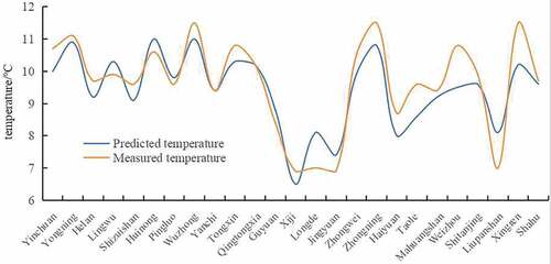
The curves of the observed and the simulated annual average temperatures in 2016 are shown in Figure 4 and were found to be in good agreement. In particular, the accuracies of the simulated annual average temperatures in Yanchi, Yongning, Pingluo, Qingtongxia, Mahuangshan, Shitanjing, and Shahu were the highest.

Figure 4. Curves of the observed and simulated annual average temperatures in 2016 at 25 stations in Ningxia.

Accuracy of the Simulated Temperature

The annual average temperature in each meteorological station in Ningxia in 2016 was simulated by separately using the CNN and the LSTM models. The values of R² of the simulated and measured annual average temperatures obtained by the CNN, LSTM, and CNN-LSTM were calculated. The spatial distribution of R² was obtained by using the Kriging interpolation method to validate the performance of the CNN-LSTM model (Figure 5).

Figure 5. Spatial distribution of R² between the measured and the simulated temperatures in 2016, as obtained by the CNN (a), LSTM (b), and CNN-LSTM (c).

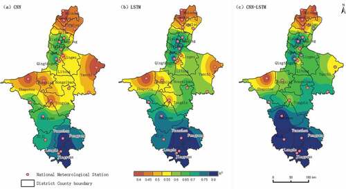
The accuracies of the simulated average temperature obtained by using the CNN, LSTM, and CNN-LSTM had similar spatial distribution. The values of R² in the south of Ningxia, such as Jingyuan, Longde, and Pengyang, were large because these areas are mountainous and hilly, with a low annual average temperature and annual difference in temperature. The values of R² in central Ningxia, such as in Xingqing, Xixia, and Jinfeng, were large. It is because the blocking of the cold westerly winds by the Helan Mountains on the western edge of this region in winter increased the air temperature and led to a smaller difference in temperature than in the other regions. In addition, the dense distribution of meteorological stations in this region can lead to a high accuracy of spatial interpolation. Small values of R² were mainly distributed in the northern, eastern, and western marginal areas of Ningxia, such as Pingluo, Huinong, Dawukou, Shapotou, and Yanchi. Small values of R² were also obtained in the west and east of Ningxia because these areas are located along the edge of the Tengger Desert and the Mu Us Desert, respectively, with large differences in the annual and daily temperatures. The reason for small values of R² in the north is unknown, and needs to be further studied.

Spatial differentiation is prominent among the accuracies of the simulated average temperature obtained from the CNN, LSTM, and CNN-LSTM. The CNN yielded the smallest area for which the temperature was simulated highly accurately (R² ≥ 0.75) and was mainly distributed in Jingyuan, Longde, Pengyang, and Yuanzhou. It also had the largest area for which the temperature was predicted with a poor accuracy (R² ≤ 0.45), and was mainly distributed in Huinong, Dawukou, Pingluo, Shapotou, Yanchi, Zhongning, and Tongxin. The area for which the temperature was predicted highly accurately (R² ≥ 0.75) by the LSTM was larger than that for the CNN, and was mainly distributed in Jingyuan, Longde, Pengyang, Yuanzhou, Xiji, and Haiyuan. The LSTM also had a smaller area than the CNN for which its accuracy was poor (R² ≤ 0.45), and this was mainly distributed in Huinong, Dawukou, Shapotou, and Yanchi. The CNN-LSTM recorded the largest area for which the predicted temperature was highly accurate (R² ≥ 0.75) and was mainly distributed in Jingyuan, Longde, Pengyang, Xiji, Yuanzhou, Haiyuan, Xixiat, Xingqing, Jinfeng, Tongxin, Yongning, and Yanchi. It also had the smallest area for which its accuracy was poor (R² ≤ 0.45), and this was mainly distributed in Huinong, Dawukou, and Shapotou. Therefore, simulations by the CNN-LSTM yielded the highest accuracy and the CNN delivered the worst.

The differences in the spatial distributions of the accuracy of the simulated average temperature obtained by using the CNN, LSTM, and CNN-LSTM may be related to their structures. The CNN-LSTM model can store information in a long-term memory unit, and this has a positive effect on the simulation of complex time series data for temperature. On the contrary, the CNN had the lowest accuracy owing to the lack of a structured memory. The input gate, forgetting gate, and output gate of the LSTM could adequately process long-time temperature data, because of which its simulated temperature was more accurate than that simulated by the CNN.

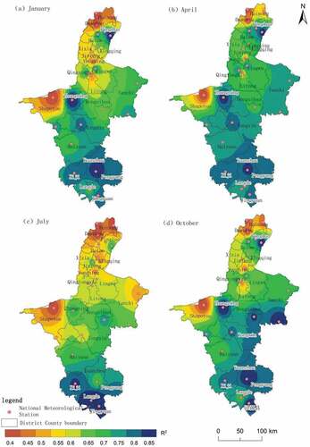
The monthly average temperatures in January, April, July, and October in 2016, representing winter, spring, summer, and autumn, respectively, were simulated by using the CNN-LSTM model to further assess its performance. The values of R² of the monthly average temperatures in January, April, July, and October were calculated. The spatial distributions of R² in the four months were obtained by using spatial Kriging interpolation (Figure 6). In winter (January), the temperature over a large area was highly accurately simulated by the CNN-LSTM (R² ≥ 0.8), and was mainly distributed in Yuanzhou, Pengyang, Xiji, Jingyuan, Zhongning, and Pingluo. The area that was highly accurately simulated by it in spring (April) (R² ≥0.8) was the largest, and was mainly distributed in Pingluo, Zhongning, Tongxin, Yanchi, Haiyuan, Yuanzhou, Xiji, Pengyang, and Jingyuan. The proposed method accurately simulated the temperature in the smallest area in summer (July) (R² ≥ 0.8), and this was mainly distributed in Jingyuan, Longde, Pengyang, and Xiji. The accuracy of simulation in autumn (October) was similar to that in spring. The areas for which the temperature was predicted highly accurately (R² ≥ 0.8) were mainly distributed in Pingluo, Zhongning, Yuanzhou, Pengyang, Jingyuan, Tongxin, Yanchi, and Xiji. Therefore, the CNN-LSTM obtained the highest accuracy of the simulated monthly average temperature in spring and autumn, followed by winter, and the lowest in summer. The accuracies of the simulated temperature in different months might have been related to the different factors influencing the changes in temperature in these months, and this needs to be further studied.

Figure 6. Distributions of R² of the monthly mean temperatures in January (a), April (b), July (c), and October (d) in 2016, as simulated by the CNN-LSTM.

Temperature Prediction

The year 2020 was selected as the base year, and the climate was assumed to be stable in the next five years. The values of key meteorological elements, such as the daily average, minimum, and maximum temperatures, rainfall, sunshine hours, and wind speed, were input to the CNN-LSTM model to predict the annual average temperatures at the 25 meteorological stations in Ningxia in the next five years. The Kriging method was used to spatially interpolate the predicted annual average temperature at each meteorological station in Ningxia from 2021 to 2025 (Figure 7).

Figure 7. Spatial distributions of the annual average temperatures from 2021 to 2025 in Ningxia, as predicted by the CNN-LSTM according to the annual average temperature in the base year of 2020.

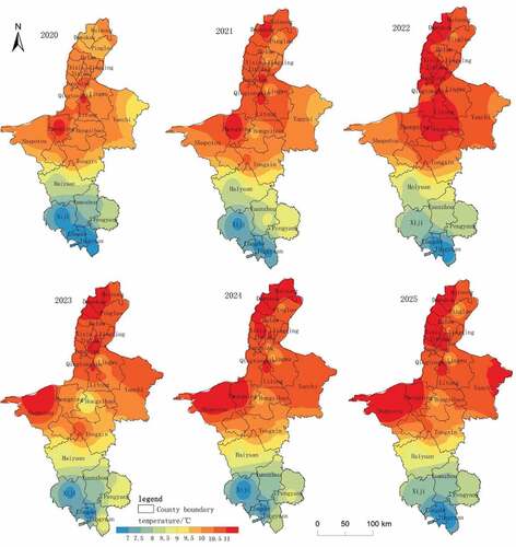
The distribution of the annual average temperature from 2020 to 2025 exhibited prominent latitudinal zonality in the south and longitudinal zonality in the north of Ningxia. The area with high annual average temperature (≥ 10.5°C) gradually increases from 2020 to 2025, compared with the distribution of the annual average temperature in the base year of 2020. The areas with a high temperature were mainly distributed in Zhongning and Litong in 2020, northwestern Ningxia in 2021, and in northern Ningxia from 2022 to 2025, as the annual average temperature increased year by year. Areas with low temperature from 2020 to 2025 (≤ 7.5°C) were mainly distributed in Liupan Mountains in southern Ningxia, and decreased year by year. Therefore, the annual average temperature in Ningxia will show an upward trend in the next five years.

Discussion

The proposed CNN-LSTM model for temperature prediction can automatically learn the relationships among the temperature, precipitation, wind field, and other meteorological elements. It can extract the characteristic information of a large number of meteorological elements at different time scales. Highly correlated meteorological elements were input to the CNN-LSTM to deal with the dispersion of data to make the model portable and efficient. Kriging interpolation method was used to obtain the spatial distribution of the simulated and predicted temperatures as well as their accuracies. These results can reflect the macro distribution of the trend of monthly and annual average temperatures according to the topographic characteristics of Ningxia. The temperature in southern Ningxia exhibited prominent latitudinal zonal differentiation while that in northern Ningxia had prominent radial zonal differentiation. The accuracy of prediction in regions with small annual variation in temperature was higher than that in areas with large variations in it. The accuracy of simulation of the temperature in spring and autumn was higher than that in summer. The predicted annual average temperature in Ningxia showed an upward trend year by year. The CNN-LSTM has a higher accuracy of simulation and prediction as well as better generalization performance than the CNN and LSTM.

The proposed deep learning model for temperature prediction is a data-driven model with nonlinear fitting. Considering more elements, such as the ocean current, terrain, and atmospheric circulation, and more meteorological stations in the province (study area) as well as its surrounding provinces, can improve the accuracy of temperature prediction and the capability of the model for generalization. In addition, too long a stride for temperature prediction can generate large cumulative errors during continuous prediction. Therefore, it is important to design a reasonable predictive stride to reduce the cumulative error in continuous prediction.

Disclosure Statement

No potential conflict of interest was reported by the authors.

Data Availability Statement

Dataset(s) derived from public resources and made available with the article. The datasets analyzed during the current study are available in the [the National Oceanic and Atmospheric Administration (NOAA) of the United States] repository. These datasets were derived from the following public domain resources: [https://psl.noaa.gov/data/gridded/tables/temperature.html; ftp://ftp.ncdc.noaa.gov/pub/data/noaa/isd-lite/]

Additional information

Funding

This work was supported by the National Natural Science Foundation of China [grant number 41661026] and the Natural Science Foundation of Ningxia Province in China [grant number 2022AAC03055].

References

- Abdel-Aal, R. E. 2004. Hourly temperature forecasting using abductive networks. Engineering Applications of Artificial Intelligence 17 (5):543–217. doi:10.1016/j.engappai.2004.04.002.
- Abdolrasol, M. G. M., S. M. S. Hussain, T. S. Ustun, M. R. Sarker, M. A. Hannan, R. Mohamed, J. A. Ali, S. Mekhilef, and A. Milad. 2021. Artificial neural networks based optimization techniques: A review. Electronics 10 (21):2689. doi:10.3390/electronics10212689.
- Abramson, B., J. Brown, W. Edwards, A. Murphy, and R. L. Winkler. 1996. Hailfinder: A Bayesian system for forecasting severe weather. International Journal of Forecasting 12 (1):57–71. doi:10.1016/0169-2070(95)00664-8.
- Asha, J., K. S. Santhosh, and S. Rishidas. 2021. Forecasting performance comparison of daily maximum temperature using ARMA based methods. Journal of Physics: Conference Series 1921 (1):012041. doi:10.1088/1742-6596/1921/1/012041.
- Astsatryan, H., H. Grigoryan, A. Poghosyan, R. Abrahamyan, S. Asmaryan, V. Muradyan, G. Tepanosyan, Y. Guigoz, and G. Giuliani. 2021. Air temperature forecasting using artificial neural network for Ararat valley. Earth Science Informatics 14 (2):711–22. doi:10.1007/s12145-021-00583-9.
- Byeongseong, C., B. Mario, B. Z. Elie, and P. Matteo. 2021. Short-term probabilistic forecasting of meso-scale near-surface urban temperature fields. Environmental Modelling & Software 145 (11):105189. doi:10.1016/j.envsoft.2021.105189.
- Carrión, D., K. B. Arfer, J. Rush, M. Dorman, S. T. Rowland, M. A. Kioumourtzoglou, I. Kloog, and A. C. Just. 2021. A 1-km hourly air-temperature model for 13 northeastern U.S. states using remotely sensed and ground-based measurements. Environmental Research 200:111477. doi:10.1016/j.envres.2021.111477.
- Chevalier, R. F., G. Hoogenboom, R. W. Mcclendon, and J. A. Paz. 2011. Support vector regression with reduced training sets for air temperature prediction: A comparison with artificial neural networks. Neural Computing & Applications 20 (1):151–59. doi:10.1007/s00521-010-0363-y.
- Cifuentes, J., G. Marulanda, A. Bello, and J. Reneses. 2020. Air temperature forecasting using machine learning techniques: A review. Energies, MDPI 13 (16):1–28. doi:10.3390/en13164215.
- Gautier, C., P. Peterson, and C. Jones. 1998. Ocean surface air temperature derived from multiple data sets and artificial neural networks. Geophysical Research Letters 25 (22):4217–20. doi:10.1029/1998GL900086.
- Gos, M., J. Krzyszczak, P. Baranowski, M. Murat, and I. Malinowska. 2020. Combined TBATS and SVM model of minimum and maximum air temperatures applied to wheat yield prediction at different locations in Europe. Agricultural and Forest Meteorology 281:107827. doi:10.1016/j.agrformet.2019.107827.
- Hanoon, M. S., A. N. Ahmed, N. Zaini, A. Razzaq, P. Kumar, M. Sherif, A. Sefelnasr, and A. ElShafie. 2021. Developing machine learning algorithms for meteorological temperature and humidity forecasting at Terengganu state in Malaysia. Scientific Reports 11 (1): 18935–18935. doi:10.1038/s41598-021-96872-w.
- Hernández-Travieso, J. G., A. G. Ravelo-García, J. B. Alonso-Hernández, and C. M. Travieso-González. 2020. Neural networks fusion for temperature forecasting. Neural Computing & Applications 32 (20):15699–710. doi:10.1007/s00521-018-3450-0.
- Hou, J. W., Y. J. Wang, J. Zhou, and Q. Tian. 2022. Prediction of hourly air temperature based on CNN–LSTM. Geomatics, Natural Hazards and Risk 13 (1):1962–86. doi:10.1080/19475705.2022.2102942.
- Jeong, S., I. Park, H. S. Kim, C. H. Song, and H. K. Kim. 2021. Temperature prediction based on bidirectional long short-term memory and convolutional neural network combining observed and numerical forecast data. Sensors 21 (3):941. doi:10.3390/s21030941.
- Krasnopolsky, V. M., and M. S. Fox-Rabinovitz. 2006. Complex hybrid models combining deterministic and machine learning components for numerical climate modeling and weather prediction. Neural Networks 19 (2):122–34. doi:10.1016/j.neunet.2006.01.002.
- Lin, M. L., C. W. Tsai, and C. K. Chen. 2021. Daily maximum temperature forecasting in changing climate using a hybrid of multi-dimensional complementary ensemble empirical mode decomposition and radial basis function neural network. Journal of Hydrology: Regional Studies 38 (12):100923. doi:10.1016/j.ejrh.2021.100923.
- Liu, Z., W. Zhan, J. Lai, F. Hong, J. Quan, B. Bechtel, F. Huang, and Z. Zou. 2019. Balancing prediction accuracy and generalization ability: A hybrid framework for modelling the annual dynamics of satellite-derived land surface temperatures. ISPRS Journal of Photogrammetry and Remote Sensing 151:189–206. doi:10.1016/j.isprsjprs.2019.03.013.
- Livera, A. M. D., R. J. Hyndman, and R. D. Snyder. 2011. Forecasting time series with complex seasonal patterns using exponential smoothing. Journal of the American Statistical Association 106 (496):1513–27. doi:10.1198/jasa.2011.tm09771.
- Maqsood, I., M. Khan, and A. Abraham. 2004. An ensemble of neural networks for weather forecasting. Neural Computing & Applications 13 (2):112–22. doi:10.1007/s00521-004-0413-4.
- Mba, L., P. Meukam, and A. Kemajou. 2016. Application of artificial neural network for predicting hourly indoor air temperature and relative humidity in modern building in humid region. Energy and Buildings 121:32–42. doi:10.1016/j.enbuild.2016.03.046.
- Milad, A., I. Adwan, S. A. Majeed, N. I. M. Yusoff, N. Al-Ansari, and Z. M. Yaseen. 2021. Emerging technologies of deep learning models development for pavement temperature prediction. IEEE Access 9:23840–49. doi:10.1109/ACCESS.2021.3056568.
- Mtibaa, F., K. K. Nguyen, M. Azam, A. Papachristou, J. S. Venne, and M. Cheriet. 2020. LSTM-based indoor air temperature prediction framework for HVAC systems in smart buildings. Neural Computing & Applications 32 (23):17569–85. doi:10.1007/s00521-020-04926-3.
- Murat, M., I. Malinowska, M. Gos, and J. Krzyszczak. 2018. Forecasting daily meteorological time series using ARIMA and regression models. International Agrophysics 32 (2):253–64. doi:10.1515/intag-2017-0007.
- Murat, M., I. Malinowska, H. Hoffmann, and P. Baranowski. 2016. Statistical modelling of agrometeorological time series by exponential smoothing. International Agrophysics 30 (1):57–65. doi:10.1515/intag-2015-0076.
- Murthy, K. V. N., R. Saravana, G. K. Kumar, and K. V. Kumar. 2021. Modelling and forecasting for monthly surface air temperature patterns in India, 1951–2016: Structural time series approach. Journal of Earth System Science 130 (1):21. doi:10.1007/s12040-020-01521-x.
- Nury, A. H., K. Hasan, and M. J. B. Alam. 2017. Comparative study of wavelet-ARIMA and wavelet-ANN models for temperature time series data in northeastern Bangladesh. Journal of King Saud University - Science 29 (1):47–61. doi:10.1016/j.jksus.2015.12.002.
- Ortiz-Garcia, E. G., S. Salcedo-Sanz, C. Casanova-Mateo, A. Paniagua-Tineo, and J. A. Portilla-Figueras. 2012. Accurate local very short-term temperature prediction based on synoptic situation support vector regression banks. Atmospheric Research 107:1–8. doi:10.1016/j.atmosres.2011.10.013.
- Prior, M. J., and M. C. Perry. 2014. Analyses of trends in air temperature in the United Kingdom using gridded data series from 1910 to 2011. International Journal of Climatology 34 (14):3766–79. doi:10.1002/joc.3944.
- Radhika, Y., and M. Shashi. 2009. Atmospheric temperature prediction using support vector machines. International Journal of Computer Theory and Engineering 1 (1):55–58. doi:10.7763/IJCTE.2009.V1.9.
- Ramesh, K., and R. Anitha. 2014. Marspline model for lead seven-day maximum and minimum air temperature prediction in Chennai, India. Journal of Earth System Science 123 (4):665–72. doi:10.1007/s12040-014-0434-z.
- Şahin, M. 2012. Modelling of air temperature using remote sensing and artificial neural network in Turkey. Advances in Space Research 50 (7):973–85. doi:10.1016/j.asr.2012.06.021.
- Sebastian, K., C. Bartosz, K. Leszek, and G. M. de Caracas. 2018. Air temperature forecasts’ accuracy of selected short-term and long-term numerical weather prediction models over Poland. Geofizika 35 (1):67–85. doi:10.15233/gfz.2018.35.5.
- Sekertekin, A., M. Bilgili, N. Arslan, A. Yildirim, K. Celebi, and A. Ozbek. 2021. Short-term air temperature prediction by adaptive neuro-fuzzy inference system (ANFIS) and long short-term memory (LSTM) network. Meteorology and Atmospheric Physics 133 (3):943–59. doi:10.1007/s00703-021-00791-4.
- Stelian, C., T. Camille, T. B. M. J. Ouarda, C. Fateh, and N. S. Dabo. 2019. Short-term air temperature forecasting using nonparametric functional data analysis and SARMA models. Environmental Modelling & Software 111 (1):394–408. doi:10.1016/j.envsoft.2018.09.017.
- Sun, Y., X. Yao, X. Bi, X. Huang, X. Zhao, and B. Qiao. 2021. Time-series graph network for sea surface temperature prediction. Big Data Research 25:100237. doi:10.1016/j.bdr.2021.100237.
- Tasadduq, I., S. Rehman, and K. Bubshait. 2002. Application of neural networks for the prediction of hourly mean surface temperatures in Saudi Arabia. Renewable Energy 25 (4):545–54. doi:10.1016/S0960-1481(01)00082-9.
- Tran, T. T. K., S. M. Bateni, S. J. Ki, and H. Vosoughifar. 2021. A review of neural networks for air temperature forecasting. Water 13 (9): 1294−1294. doi:10.3390/w13091294.
- Ustaoglu, B., H. K. Cigizoglu, and M. Karaca. 2008. Forecast of daily mean, maximum and minimum temperature time series by three artificial neural network methods. Meteorological Applications 15 (4):431–45. doi:10.1002/met.83.
- Xiao, C., N. Chen, C. Hu, K. Wang, and Z. Chen. 2019. Short and mid-term sea surface temperature prediction using time-series satellite data and LSTM-Adaboost combination approach. Remote Sensing of Environment 233:111358. doi:10.1016/j.rse.2019.111358.
- Ye, L., G. Yang, E. V. Ranst, and H. Tang. 2013. Time-series modeling and prediction of global monthly absolute temperature for environmental decision making. Advances in Atmospheric Sciences 30 (2):382–96. doi:10.1007/s00376-012-1252-3.
- Y. J., Wang. 2022. Spatiotemporal temperature prediction based on CNN-LSTM and meteorological element correlation (Ningxia University (In Chinese)). https://webvpn.nxu.edu.cn/https/77726476706e69737468656265737421fbf952d2243e635930068cb8/kcms/detail/detail.aspx?dbcode=CMFD&dbname=CMFDTEMP&filename=1022054517.nh&uniplatform=NZKPT&v=fv_ws6hsUFqxuC8SZt546Zsv8i7iE5v9zpiD8hIyMncrbxIxjBajN_u1S66ikBCV
- Yu, X., S. X. Shi, and L. Y. Xu. 2021. A spatial–temporal graph attention network approach for air temperature forecasting. Applied Soft Computing 113:107888. doi:10.1016/j.asoc.2021.107888.
- Zhang, Z., Y. Dong, and Y. Yuan. 2020. Temperature forecasting via convolutional recurrent neural networks based on time-series data. Complexity 2020:1–8. doi:10.1155/2020/3536572.
- Zhang, X., Q. Zhang, G. Zhang, Z. Nie, Z. Gui, and H. Que. 2018. A novel hybrid data-driven model for daily land surface temperature forecasting using long short-term memory neural network based on ensemble empirical mode decomposition. International Journal of Environmental Research and Public Health 15 (5):1032. doi:10.3390/ijerph15051032.