Fuzzy model-based sparse clustering with multivariate t-mixtures

ABSTRACT

Model-based clustering technique is an optimal choice for the distribution of data sets and to find the real structure using mixture of probability distributions. Many extensions of model-based clustering algorithms are available in the literature for getting most favorable results but still its challenging and important research objective for researchers. In the model-based clustering, many proposed methods are based on EM algorithm to overcome its sensitivity and initialization. However, these methods treat data points with feature (variable) components under equal importance, and so cannot distinguish the irrelevant feature components. In most of the cases, there exist some irrelevant features and outliers/noisy points in a data set, upsetting the performance of clustering algorithms. To overcome these issues, we propose a fuzzy model-based t-clustering algorithm using mixture of t-distribution with an $L_1$regularization for the identification and selection of better features. In order to demonstrate its novelty and usefulness, we apply our algorithm on artificial and real data sets. We further used our proposed method on soil data set, which was collected in collaboration with and the assistance of Environmental laboratory Karakoram International University (GB) from various point/places of Gilgit Baltistan, Pakistan. The comparison results validate the novelty and superiority of our newly proposed method for both the simulated and real data sets as well as effectiveness in addressing the weaknesses of existing methods.

Introduction

The most common obstacle in machine learning and pattern recognition is to divide intrinsic structure of given data set into similar group, which is famously known as clustering (Jain and R, 1988; Mcnicholas, 2016). Cluster analysis, also known as unsupervised learning, is one of the most significant and successfully employed techniques that has noteworthy application in various areas such as wireless networking and Remote Sensing (Abbasi and Younis, 2007; Gogebakan and Erol, 2018), computational biology (Gogebakan, 2021; Yang and Ali, 2019), imaging processing (Chuang et al., 2006), soft computing (Gogebakan, 2021), data segmentation (Gogebakan and Hamza 2019), agriculture (Kadim and Wirnhardt, 2012), ecology (Rasool et al., 2016), data mining (Agrawal et al.,2005) and economics (Garibaldi et al., 2006) etc. There are two major areas of clustering algorithms, namely, model-based clustering and nonparametric approach (McLachlan and Basford, 1988). For nonparametric approach, clustering methods are based on objective functions where K-Mean, Fuzzy C-mean and Possibilistic C mean are most common. In model-based clustering approach, we consider that the data points follow a mixture of probability distribution (Banfield and Raftery, 1993) where the EM (Expectation-Maximization) algorithm proposed by Dempster et al. (1977) is the most common and famous approach using maximum-likelihood estimation for inferring mixture models (Biernacki and Jacques, 2013; Lee and Scott,2012; Melnykov and Melnykov, 2012; Yang et al., 2012). A large number of algorithms have been proposed in model-based clustering, among them Yang and Ali (2019), Banfield and Raftery (1993), Yang, Chang-Chien, and Nataliani (2019), Yang et al. (2014), Fraley andRaftery (2002), Lo and Gottardo (2012) are most famous methods. Feature selection is not only the important technique in clustering but also challenging for researchers to get most relevant features. Due to the presence of irrelevant features in data sets, many complexities arise during clustering. Among those first is, clustering without relevant feature selection may fail to find the real structure of data and provide a minimum accuracy rate. Secondly, for high-dimensional data sets, clustering is computationally infeasible in the presence of irrelevant features. Thirdly, the presence of irrelevant features may also cause an appropriate model selection criterion problem. In addition, removing non-informative features may largely enhance interpretability (Pan and Shen, 2007; Xie et al., 2007). In this connection, Tibshirani (1996) introduced the idea of Lasso regularization to cope up with sparsity in the context of regression analysis. Zadeh (1965) presented the idea of fuzzy set which is useful in many areas.

In 2014, Yang et al. (2014) have presented the idea of robust fuzzy classification maximum likelihood using multivariate t-distribution (FCML-T). Although this method is simple and applicable for noisy points and/or outliers in data sets but not applicable for irrelevant features selection. In 2019, Yang and Ali (2019) have presented the idea of fuzzy Gaussian mixture model for feature selection using Lasso regularization but we are familiar that due to shorter tail of normal distribution in many cases, it is not an appropriate choice for clustering. Furthermore, it does not provide us robust results specially when the data sets have outliers or noisy points. To overcome these issues (due to outliers and/or noisy points), we extended the fuzzy classification maximum likelihood t-distribution using Lasso regularization and we called it F-MT-Lasso clustering algorithm. To show the novelty and usefulness of our proposed algorithm (F-MT-Lasso), we use simulated as well as real data sets and compare the performance of our proposed algorithm F-MT-Lasso with that of fuzzy model-based Gaussian clustering (F-MB-N) (Yang, Chang-Chien, and Nataliani 2019), FCML-T (Yang et al.,2014) and Fuzzy Gaussian Lasso algorithm (Yang and Ali, 2019) algorithms. Results show the significance and upper hand of our proposed F-MT-Lasso algorithm. The rest of paper is organized as follows. In section 2, we discuss our proposed model fuzzy t-clustering Lasso algorithm. Section 3 elaborates the comparative analysis of our proposed method with some of existing schemas using simulated and real data sets. In section 4, we apply our algorithm on a real data set from field of biosciences. Section 5 details the application of our algorithm on real data set regarding soil which was collected from various placed of Gilgit-Baltistan, Pakistan in collaboration with of Karakoram International University Gilgit-Baltistan, Pakistan. We summarized our conclusions in section 6.

Fuzzy T-Distribution Lasso Clustering

Let a p-dimensional random variable X follows multivariate t-distribution with probability density function$f_t(x_i;{\mu }_k,\sum _k,v_k)$. Where${\mu }_k$,$\sum _k$, and $v_k$ are mean, covariance and degree of freedom, respectively. The multivariate t-distribution is as follows:

$f_t(x_i;{\mu }_k,{\displaystyle \sum _k,}{v}_k)=\Gamma \frac{v+p}{2}{\left(\pi v\right)}^{\frac{p}{2}}\Gamma \frac{v}{2}\sum \frac{1}{2}{\left\{1+\frac{{(x-\mu )}^T{{\displaystyle \sum }}^{-1}(x-\mu )}{v}\right\}}^{\frac{v+p}{2}}$, where $(x-\mu {)}^T\sum ^{-1}(x-\mu )$ is mahalonobis square distance between data points $x$ and the mean$(\mu )$,is the covariance matrix, and $\mathrm{\Gamma }\left(\mathrm{v}\right)$ is the Gamma function with $\mathrm{\Gamma }=\underset{0}{\overset{\mathrm{\infty }}{\int }}{s}^{v-1}{e}^{-s}ds$. In 1965 Zadeh (1965) presented the idea of fuzzy set and Yang et al., (2014) proposed the idea of fuzzy classification maximum likelihood clustering (FCML-T) and the objective function is as follows: $J(z,\alpha ,\theta )=\sum _{i=1}^n\sum _{k=1}^c{z}_{ki}^{m}ln(f(x_i;\theta )+w\sum _{i=1}^n\sum _{k=1}^c{z}_{ki}^{m}ln{\alpha }_k$. Here we consider$\theta =\left\{{\mu }_k,\sum _k,v_k\right\}$. In the objective function$J(z,\alpha ,\theta )$,$m$ is fuzziness index, $m\in (1,\mathrm{\infty })$and $w\ge 0$ are fixed constants and ${\alpha }_k$ are mixing proportions and must satisfying $0\le {\alpha }_k\le 1$ while sum to one. We extend the fuzzy classification maximum likelihood proposed by Yang et al., (2014) with multivariate t-distribution using Lasso penalty term using common diagonal variances. As we know that mixture of multivariate t-distribution is considered as a scale mixture of normal distributions. Suppose Y is latent variable then $x|y\sim N(x;\mu ,{\sum }^{/}y)$with$Y\sim G\left(\frac{v_k}{2},\frac{v_k}{2}\right)$,where the gamma density function is defined as; $f(y;A,B)=\left\{B^A{y}^{A-1}/\mathrm{\Gamma }(A)\right\}exp(-By)I_{(0,\mathrm{\infty })}(y);$ and $(A,B>0).$So we can write the objective function as $J(z,\alpha ,\theta )=\sum _{i=1}^n\sum _{k=1}^c{z}_{ki}^{m}ln[N(x;\mu ,{\sum }^{/}{y}_{ki})G(y_{ki};v_k/2,v_k/2)]+w\sum _{i=1}^n\sum _{k=1}^c{z}_{ki}^{m}ln{\alpha }_k$.

We further extend fuzzy classification maximum likelihood clustering algorithm proposed by Yang et al., (2014) into a new method of multivariate t-distribution by adding the term$\lambda \sum _{k=1}^c\sum _{p=1}^p\left|{\mu }_{kp}\right|$. Thus, we propose a new F-MT-Lasso objective function as follows:

$J_{\mathrm{F}-\mathrm{M}\mathrm{T}-Lasso}(z,\alpha ,\theta )=\sum _{i=1}^n\sum _{k=1}^c{z}_{ki}^{m}ln[N(x;\mu ,{\sum }^{/}{y}_{ki})G(y_{ki};v_k/2,v_k/2)]+w\sum _{i=1}^n\sum _{k=1}^c{z}_{ki}^{m}ln{\alpha }_k-\lambda \sum _{k=1}^c\sum _{p=1}^p\left|{\mu }_{kp}\right|$

where $\lambda \ge 0$is tuning parameter that manage the amount of shrinkage and mean parameter. When the value of tuning parameter$\lambda$is sufficiently large, some of the cluster centers $({\mu }_{kp})$to be exactly zero and we discard the features when${\mu }_{kp}=0$.We use common diagonal covariance${\mathrm{\Sigma }}_k={\sum }^{=}{\sigma }_p^2$, and$w^{(t)}={0.999}^{(t)}$.To get the necessary conditions for minimizing the F-MT-Lasso objective function, we use the lagrangian as follows:

$J_{\mathrm{F}-\mathrm{M}\mathrm{T}-Lasso}(z,\alpha ,\theta )=\sum _{i=1}^n\sum _{k=1}^c{z}_{ki}^{m}lnf\left(x_i;\theta \right)+w\sum _{i=1}^n\sum _{k=1}^c{z}_{ki}^{m}ln{\alpha }_k-\lambda \sum _{k=1}^c\sum _{p=1}^p\left|{\mu }_{kp}\right|-\gamma \left(\sum _{k=1}^c{z}_{ki}-1\right)-\beta \left(\sum _{k=1}^c{\alpha }_k-1\right).$

The necessary conditions of$y_{ki}$to maximize $J_{\mathrm{F}-\mathrm{M}\mathrm{T}-\mathrm{L}\mathrm{a}\mathrm{s}\mathrm{s}\mathrm{o}}(z,\alpha ,\theta )$ are as follows:

(1) $y_{ki}=\frac{(v_k+d-2)}{\left\{{(x_i-{\mu }_k)}^T{\sum }_k^{-1}(x_i-{\mu }_k)+v_k\right\}}$(1)

Differentiate $J_{\mathrm{F}-\mathrm{M}\mathrm{T}-\mathrm{L}\mathrm{a}\mathrm{s}\mathrm{s}\mathrm{o}}(z,\alpha ,\theta )$ with respect to the fuzzy membership function, $z_{ki}$, we obtain the updating equation for the membership function as follows:

(2) ${\hat{z}}_{ki}=\frac{{(lnf(x_i;\theta )+wln({\alpha }_k))}^{-\frac{1}{m-1}}}{\sum _{s=1}^c{(lnf(x_i;\theta )+wln({\alpha }_k))}^{-\frac{1}{m-1}}}$(2)

Differentiate $J_{\mathrm{F}-\mathrm{M}\mathrm{T}-\mathrm{L}\mathrm{a}\mathrm{s}\mathrm{s}\mathrm{o}}(z,\alpha ,\theta )$ w.r.t ${\alpha }_k$ we obtain the value of mixing proportion ${\hat{\alpha }}_k$

(3) ${\hat{\alpha }}_k=\frac{\sum _{i=1}^n{z}_{ki}^m}{\sum _{k=1}^c\sum _{i=1}^n{z}_{ki}^m}$(3)

For the degree of freedom, we differentiate $J_{\mathrm{F}-\mathrm{M}\mathrm{T}-\mathrm{L}\mathrm{a}\mathrm{s}\mathrm{s}\mathrm{o}}(z,\alpha ,\theta )$ with respect to$v_k$.We obtain the following equation:

(4) $ln\left(\frac{v_k}{2}\right)-\psi \left(\frac{v_k}{2}\right)+1+\frac{\sum _{i=1}^n{z}_{ki}^m(ln{y}_{ki}-y_{ki})}{\sum _{i=1}^n{z}_{ki}^m}=0$(4)

where $\psi (u)$ is the digamma function $\psi (u)=\frac{d}{du}ln\mathrm{\Gamma }u$, We used decreasing learning parameter $w$ as: $w^{\left(t\right)}={0.999}^t$

(5) $w^{\left(t\right)}={0.999}^t$(5)

To get the updating equation of ${\mu }_{kp}$we differentiate $J_{\mathrm{F}-\mathrm{M}\mathrm{T}-\mathrm{L}\mathrm{a}\mathrm{s}\mathrm{s}\mathrm{o}}(z,\alpha ,\theta )$ with respect to ${\mu }_{kp}$ we obtain the estimated value of ${\hat{\mu }}_{kp}$

(6) $\begin{array}{rl}& {\hat{\mu }}_{kp}=\left\{\begin{array}{c}{\tilde{\mu }}_{kp}+\frac{\lambda {\hat{\sigma }}_p^2}{{\sum }_{i=1}^n{\hat{z}}_{ki}^m{y}_{ki}},if{\tilde{\mu }}_{kp}<-\frac{\lambda {\hat{\sigma }}_p^2}{{\sum }_{i=1}^n{\hat{z}}_{ki}^m{y}_{ki}}\\ 0,if\left|c\right|\le \frac{\lambda {\hat{\sigma }}_p^2}{{\sum }_{i=1}^n{\hat{z}}_{ki}^m{y}_{ki}}\\ {\tilde{\mu }}_{kp}-\frac{\lambda {\hat{\sigma }}_p^2}{{\sum }_{i=1}^n{\hat{z}}_{ki}^m{y}_{ki}},if{\tilde{\mu }}_{kp}>\frac{\lambda {\hat{\sigma }}_p^2}{{\sum }_{i=1}^n{\hat{z}}_{ki}^m{y}_{ki}}\end{array}\right.\\ & \end{array}$(6)

With having

(7) ${\tilde{\mu }}_{kp}=\frac{\sum _{i=1}^n{z}_{ki}^m{y}_{ki}{x}_{ip}}{\sum _{i=1}^n{z}_{ki}^m{y}_{ki}}$(7)

where ${\tilde{\mu }}_{kp}=\sum _{i=1}^n{z}_{ki}^m{y}_{ki}{x}_{ip}/\sum _{i=1}^n{z}_{ki}^m{y}_{ki}$ is the maximum likelihood estimator (MLE) of the FCML-T clustering and ${\mathrm{\Sigma }}_k=\sum ={\sigma }_p^2$ is common diagonal variance. When the value of $\lambda$ is sufficiently increase in Eq. (6), it should have some ${\hat{\mu }}_{kp}$ = 0, otherwise it has the quantity $\lambda {\hat{\sigma }}_p^2/\sum _{i=1}^n{z}_{ki}^m{y}_{ki}$ of shrinkage. Consequently, when we found, if$\tilde{\mu }kp\le \lambda {\widehat{\sigma }}_p^2/{\displaystyle \sum _{i=1}^n{z}_{ki}^m}{y}_{ki}$, then we consider ${\hat{\mu }}_{kp}$ = 0, and $pth$ features supposed to be uninformative and discarded it from further clustering results; otherwise, cluster center will be ${\hat{\mu }}_{kp}$=${\tilde{\mu }}_{kp}-\lambda {\hat{\sigma }}_p^2/\sum _{i=1}^n{z}_{ki}^m{y}_{ki}$. To drive the updating equation of ${\hat{\mu }}_{kp}$, we use the F-MT-Lasso objective function$J_{\mathrm{F}-\mathrm{M}\mathrm{T}-\mathrm{L}\mathrm{a}\mathrm{s}\mathrm{s}\mathrm{o}}(z,\alpha ,\theta )$.Differentiate $J_{\mathrm{F}-\mathrm{M}\mathrm{T}-\mathrm{L}\mathrm{a}\mathrm{s}\mathrm{s}\mathrm{o}}(z,\alpha ,\theta )$ with respect to ${\mu }_{kp}$,we obtain the following form:

$\frac{\mathrm{\partial }{J}_{\mathrm{F}-\mathrm{M}\mathrm{T}-\mathrm{L}\mathrm{a}\mathrm{s}\mathrm{s}\mathrm{o}}(z,\alpha ,\theta )}{\mathrm{\partial }{\mu }_{kp}}=\frac{\sum _{i=1}^n{z}_{ki}^m{y}_{ki}(x_i-{\mu }_{kp})}{{\sigma }_p^2}-\lambda sign({\mu }_{kp})$. Set $\frac{\mathrm{\partial }{J}_{\mathrm{F}-\mathrm{M}\mathrm{T}-\mathrm{L}\mathrm{a}\mathrm{s}\mathrm{s}\mathrm{o}}(z,\alpha ,\theta )}{\mathrm{\partial }{\mu }_{kp}}$ = 0, after simplification we obtain;

${\hat{\mu }}_{kp}={\tilde{\mu }}_{kp}-\frac{\lambda {\sigma }_p^{2}sign({\hat{\mu }}_{kp})}{\sum _{i=1}^n{\hat{z}}_{ki}^{(m)}{y}_{ki}}$. In mathematics, we know that some functions are not necessarily differentiable so, $\left|{\hat{\mu }}_{kp}\right|$ is not differentiable at ${\hat{\mu }}_{kp}$ = 0. Sub-derivative is defined as a set of all sub-gradients of a convex function $f$at$x$is called the sub-differential of $f$at$x$. In order to solve this problem, we use sub derivative as a substitute for the derivative. Suppose we have the absolute value function $f(x)=\left|x\right|$ at x, is the $\delta f(x)=sign(x),$ where sign function is defined as;

$sign(x)=\left\{\begin{array}{c}-1ifx<0\\ [-1,1]ifx=0\\ \left\{+1\right\}ifx>0\end{array}\right.$. The absolute function $f(x)=\left|x\right|$and its sub-differential $\delta f(x)=sign(x)$is shown in Figure 1

Figure 1. Sub-differential of $\delta f\left(x\right)=sign\left(x\right)$.

Using this concept of sub-derivative or sub-gradient, we obtained the updating Equation 7(7) ${\tilde{\mu }}_{kp}=\frac{\sum _{i=1}^n{z}_{ki}^m{y}_{ki}{x}_{ip}}{\sum _{i=1}^n{z}_{ki}^m{y}_{ki}}$(7) equation (6) for${\hat{\mu }}_{kp}$. We have considered common diagonal covariance matrix which is suitable for high dimensional data sets and good choice for feature selection in our algorithm which is explain as follows:

${\mathrm{\Sigma }}_k=\sum ={\sigma }_p^2=diag({\sigma }_p)=\left(\begin{array}{ccccc}{\sigma }_1^2& 0& 0& \cdots & 0\\ 0& {\sigma }_2^2& 0& \cdots & 0\\ 0& 0& \ddots & \hspace{0.17em}& ⋮\\ ⋮& ⋮& \hspace{0.17em}& \ddots & ⋮\\ 0& 0& \hspace{0.17em}& \cdots & {\sigma }_d^2\end{array}\right),p=1,\cdots ,d$

we differentiate objective function $J_{\mathrm{F}-\mathrm{M}\mathrm{T}-\mathrm{L}\mathrm{a}\mathrm{s}\mathrm{s}\mathrm{o}}(z,\alpha ,\theta )$ with respect to ${\sigma }_p^2,p=1,\cdots ,d$ we get the updating equation of common diagonal covariance matrix.

(8) ${\widehat{\sigma }}_p^2={\displaystyle \sum _{k=1}^c{\displaystyle \sum _{i=1}^n{z}_{ki}^m}}{y}_{ki}(x_{ip}-\mu kp)2{\displaystyle \sum _{k=1}^c{\displaystyle \sum _{i=1}^n{z}_{ki}^m}}{y}_{ki}$(8)

Thus, we have summarized our proposed F-MT-Lasso algorithm as follows:

Algorithm F-MT-Lasso clustering algorithm

Step 1: Fix$2\le c\le n$, $\epsilon >0$and$m\in (1,\mathrm{\infty })$. Give initials $w^{(0)}$=1,$v^{(0)}$ ${\alpha }_k^{(0)}$,${\mu }_{kp}^{(0)}$ , ${\sigma }_p^{2,(0)}$,$y_{ki}^{(0)}$. $\lambda =1$ and $t=1$

Step 2: Compute ${\hat{z}}_{ki}^{(0)}$ with $w^{(0)}$, ${\mu }_{kp}^{(0)}$,$y_{ki}^{(0)}$, ${\alpha }_k^{\left(0\right)}$ and ${\sigma }_p^{2,(0)}$ by Eq. (2)

Step 3: Compute ${\tilde{\mu }}_{kp}^{(t)}$with ${\hat{z}}_{ki}^{(t-1)}$and $y_{ki}^{(t-1)}$using Eq. (7).

Step 4: Compute $w^{(t)}$ using Eq. (5).

Step 5: Compute ${\hat{\alpha }}_k^{(t)}$with ${\hat{z}}_{ki}^{(t-1)}$ busing Eq. (3).

Step 6: Compute ${\hat{\sigma }}_p^{(t)2}$ with $\mu k(t)$,$y_{ki}^{(0)}$ and ${\hat{z}}_{ki}^{(t-1)}$ by (8).

Step 7: Update ${\hat{z}}_{ki}^{(t)}$ with ${\tilde{\mu }}_{kp}^{(t)}$,$y_{ki}^{(t)}$ , ${\hat{\alpha }}_k^{(t)}$ and ${\hat{\sigma }}_p^{(t)2}$ using Eq. (2).

Step 8: Compute $v_k^{(t)}$ with ${\hat{z}}_{ki}^{(t)}$and $y_{ki}^{(t-1)}$ using Eq. (4).

Step 9: Compute $y_{ki}^{(t)}$ with ${\tilde{\mu }}_{kp}^{(t)}$, $v_k^{(t)}$ and ${\hat{\sigma }}_p^{(t)2}$ using Eq. (1).

Step 10 : Update ${\tilde{\mu }}_{kp}^{(t+1)}$ with ${\hat{z}}_{ki}^{(t)}$ and $y_{ki}^{(t)}$ using Eq. (7).

If$max{\tilde{\mu }}_k^{(t+1)}-{\tilde{\mu }}_k^{(t)}<\epsilon$,stop .Else t=t+1 and return to step 3

Step 11: Update ${\hat{\sigma }}_p^{2,(t+1)}$ with${\tilde{\mu }}_{kp}^{(t+1)}$, $y_{ki}^{(t)}$ and ${\hat{z}}_{ki}^{(t)}$ using Eq. (8)

Step 12: Update ${\hat{\mu }}_{kp}^{(t)}$ with${\hat{z}}_{ki}^{(t)}$,$\mu kp(t+1)$ $y_{ki}^{(t)}$ and ${\hat{\sigma }}_{kp}^{2,(t+1)}$using Eq.(6), that is,

If $\left|{\tilde{\mu }}_{kp}^{(t+1)}\right|\le \frac{\lambda {\hat{\sigma }}_p^{2,(t+1)}}{\sum _{i=1}^n{\hat{z}}_{ki}^{m(t)}{y}_{ki}},$ then let ${\hat{\mu }}_{kp}^{(t)}$=0.

Else ${\hat{\mu }}_{kp}^{(t)}={\tilde{\mu }}_{kp}^{(t+1)}-\frac{\lambda {\hat{\sigma }}_p^{2,(t+1)}}{\sum _{i=1}^n{\hat{z}}_{ki}^{m(t)}{y}_{ki}}.$

Step 13: Increase$\lambda$ and return to Step 3, or output results.

Numerical Comparisons

Here, we demonstrate the novelty of our proposed algorithm FMT-Lasso using synthetic and real data sets by using accuracy rate define as $AR=\sum _{j=1}^k{r}_j/n$ where $r_j$ is the number of points in $C_j^{\prime }$ that are also in $C_j$ in which $C=\left\{C_1,C_2,\cdots ,C_c\right\}$ is the set of c clusters for the given data set and $C^{\prime }=\left\{C_1^{\prime },C_2^{\prime },\cdots ,C_c^{\prime }\right\}$ is the set of c clusters generated by the clustering algorithm. We compare our algorithm with F-MB-N (Yang et al. 2019b), FCML-T (Yang et al., 2014) and FG-Lasso (Yang and Ali 2019).The details of used datasets are presented in Table 1.

Table 1. Tabular repsentation of the synthetic and real data sets used.

Datasets	Samples	Variables	Clusters
Synthetic-I	1600	3	2
Synthetic-II	1050	4	3
Synthetic-III	400	3	5
Seeds	210	7	3
Pima Indian	786	8	2
Breast cancer	699	8	2
Prostate cancer	100	8	2
Soil	30	5	3

Example 1.

In this example, a two-cluster data set with 1250 data points generated from a Gaussian mixture model $\sum _{k=1}^2{\alpha }_{k}N(u_k,\sum _k)$ with the parameters ${\alpha }_k=1/2,\hspace{0.17em}\mathrm{\forall }k,$ $u_2={\left(\begin{array}{cc}20& 3\end{array}\right)}^T$and${\mathrm{\Sigma }}_1=\left(\begin{array}{cc}1& 0\\ 0& 1\end{array}\right)$,${\mathrm{\Sigma }}_2=\left(\begin{array}{cc}1& 0\\ 0& 1\end{array}\right)$. Two features, namely, $\left\{x_1,x_2\right\}$ have been added with 350 noisy points and shown in Figure 2a. Since our objective is to identify relevant features, we extend the data set from two features $\left\{x_1,x_2\right\}$up to three features$\left\{x_1,x_2,x_3\right\}$ by adding a 3^rd feature$x_3$,generated from uniform distribution over intervals [−2,2]. It implies that the third added feature$x_3$,is considered as irrelevant feature. We demonstrate F-MB-N, FCML-T, FG-Lasso and F-MT-Lasso by different initializations and record the average of 30 random initials. The clustering results of F-MB-N, FCML-T and FG-Lasso are shown in Figure 2(b-d). The final result of our proposed method F-MT-Lasso has shown in Figure 2e. Due to having irrelevant feature $x_3$ with d = 3, clustering results from different methods are highly affected and shown poor average accuracy rates, as shown in Table 2. On the other hand, our proposed method F-MT-Lasso discard non-informative feature $x_3$ and provide best average accuracy rate (AR = 0.921). The details of discarded feature through FG-Lasso and F-MT-Lasso with different values of $\lambda$ are shown in Table 3. When we increase the value of $\lambda$ from 50 to 135, we observed that FG-Lasso discard important feature$x_2$,${\hat{\mu }}_{12}={\hat{\mu }}_{22}=0$ and ${\hat{\mu }}_{13}=0$ becomes zero. Similarly, when the value of $\lambda$ is increasing up to 135, we observed that proposed method F-MT-Lasso discard ${\hat{\mu }}_{13}=0$ and ${\hat{\mu }}_{23}=0$ while FG-Lasso discards important component${\hat{\mu }}_{21}=0$. It is clearly seen that F-MT-Lasso works better and discarded third irrelevant feature$x_3$.After discarding irrelevant feature $x_3$ F-MT-Lasso shows best results, this shows the novelty of our method.

Figure 2. (a) the original 2-cluster Gaussian data set; (b) F-MB-N clustering results; (c) FCML-T clustering results; (d) FG-Lasso clustering results; (f) F-MT-Lasso clustering results.

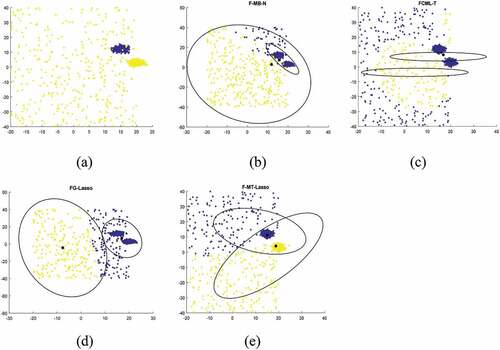
Table 2. Comparison of F-MB-N, FCML-T, FG-Lasso with F-MT-Lasso based on reduced feature and average AR.

Original features	Average AR		No of remaining features		Average AR
	F-MB-N	FCML-T	FG-Lasso	F-MT-Lasso	FG-Lasso	F-MT-Lasso
3	0.456	0.491	2	2	0.503	0.921

Table 3. Feature reduction pattern based on $\lambda$ values.

$\lambda$	Feature reduction pattern through FG-Lasso			Feature reduction pattern through F-MT-Lasso
	$x_1$	$x_2$	$x_3$	$x_1$	$x_2$	$x_3$
50	-	${\hat{\mu }}_{12}={\hat{\mu }}_{22}=0$	${\hat{\mu }}_{13}=0$	-	-	${\hat{\mu }}_{13}=0$
135	${\hat{\mu }}_{21}=0$	-	${\hat{\mu }}_{23}=0$	-	-	${\hat{\mu }}_{23}=0$

Example 2.

In this example, we consider a data set consists of 3 clusters with 950 data points generated from the Gaussian mixture (GM) distribution $\sum _{k=1}^3{\alpha }_{k}N(u_k,\sum _k)$ having parameters ${\alpha }_k=1/3,\hspace{0.17em}\mathrm{\forall }k,$ $u_1={\left(\begin{array}{cc}4& 6\end{array}\right)}^T,$ ${\mathrm{\Sigma }}_1=\left(\begin{array}{cc}3& 0\\ 0& 1\end{array}\right)$,${\mathrm{\Sigma }}_2=\left(\begin{array}{cc}1& 0\\ 0& 1\end{array}\right)$and${\mathrm{\Sigma }}_3=\left(\begin{array}{cc}1& 0\\ 0& 1\end{array}\right)$, with two feature$\left\{x_1,x_2\right\}$. We added 100 noisy points to features $\left\{x_1,x_2\right\}$using uniform distribution over the intervals [−5,5] and [0, 1], and the sample size will be 1050 points. Result is shown in Figure 3a. Since our objective is to identify relevant features, we extended the data set from 2 features $\left\{x_1,x_2\right\}$up to four features $\left\{x_1,x_2,x_3,x_4\right\}$ by adding two additional features $x_3$and$x_4$, both have been generated from uniform distribution over intervals [−1,1] and [−5, 5],it implies that the third and four added features $x_3$and $x_4$, are considered to be irrelevant features. The 3-D plots of $\left\{x_1,x_2,x_3\right\}$ and $\left\{x_1,x_2,x_4\right\}$ have shown in Figure 3(b,c). We demonstrate F-MB-N, FCML-T, FG-Lasso, and F-MT-Lasso under different initializations and record the average of 30 random initials.The clustering results of F-MB-N, FCML-T and FG-Lasso are shown in Figure 3(d-f). The final result of our proposed method F-MT-Lasso has shown in Figure 3g. Due to having irrelevant feature $x_3$and $x_4$ with d = 4, clustering results from different methods have been highly affected and shown poor average accuracy rates, as shown in Table 4. While our proposed method F-MT-Lasso discard non-informative features $x_3$ and $x_4$,as a result it provides us best average accuracy rate (AR = 0.989). The details of discarded features through FG-Lasso and F-MT-Lasso for different values of $\lambda$are shown in Table 5. When we increase the value of $\lambda$to 30, we observed that both Algorithms completely discarded irrelevant feature$x_3$. Similarly, when the value of $\lambda$is increased from 60 to 111 another irrelevant feature $x_4$ also discarded by both methods and their results have been shown in Table 5. It is clearly seen that after discarding irrelevant features $x_3$and $x_4$ our proposed algorithm shows best results.

Figure 3. (a) the original 3-cluster Gaussian data set; (b) 3-D plot representation $x_1,x_2\mathrm{a}\mathrm{n}\mathrm{d}{x}_3$ ; (c) 3-D plot representation $x_1,x_2\mathrm{a}\mathrm{n}\mathrm{d}{x}_4$ ; (d)f-MB-N clustering results; (e)fcml-T clustering results; (f)fg-Lasso clustering results; (g)f-MT-Lasso clustering results.

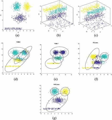
Table 4. Comparison of F-MB-N, FCML-T, FG-Lasso with F-MT-Lasso based on reduced feature and average AR.

Original feature	Average AR		No. of remaining features		Average AR
	F-MB-N	FCML-T	FG-Lasso	F-MT-Lasso	FG-Lasso	F-MT-Lasso
4	0.607	0.612	2	2	0.941	0.989

Table 5. Feature reduction pattern based on $\lambda$ values.

$\lambda$	Feature reduction pattern through FG-Lasso				Feature reduction pattern through F-MT-Lasso
	$x_1$	$x_2$	$x_3$	$x_4$	$x_1$	$x_2$	$x_3$	$x_4$
30	-	-	0	${\hat{\mu }}_{24}=0$	-	-	${\hat{\mu }}_{13}={\hat{\mu }}_{23}={\hat{\mu }}_{33}=0$	${\hat{\mu }}_{34}=0$
60	-	-	0	${\hat{\mu }}_{24}={\hat{\mu }}_{34}=0$	-	-	0	${\hat{\mu }}_{14}={\hat{\mu }}_{34}=0$
111	-	-	0	${\hat{\mu }}_{14}={\hat{\mu }}_{24}={\hat{\mu }}_{34}=0$	-	-	0	0

Example 3.

In this example, we consider a data set consists of five clusters with 400 data points generated from the Gaussian mixture (GM) distribution $\sum _{k=1}^5{\alpha }_{k}N(u_k,\sum _k)$ having parameters ${\alpha }_k=1/5,\hspace{0.17em}\mathrm{\forall }k,$ $u_1={\left(\begin{array}{cc}4& 6\end{array}\right)}^T,$ $u_5={\left(108\right)}^T,$

${\mathrm{\Sigma }}_1={\sum }_2={\sum }_3={\sum }_4={\sum }_5=\left(\begin{array}{cc}1& 0\\ 0& 1\end{array}\right)$.Two features are $\left\{x_1,x_2\right\}$ and added 400 noisy points to features $x_3$by using uniform distribution over the intervals [−10,10].Since our objective is to identify relevant features, we extended the data set from the 2 features $\left\{x_1,x_2\right\}$up to 3 features$\left\{x_1,x_2,x_3\right\}$ by adding one feature$x_3$, generated from uniform distribution over intervals [−10,10]. It implies that the third added feature$x_3$, is an irrelevant feature. The 3-D plots of $\left\{x_1,x_2,x_3\right\}$ have shown in Figure 4a. We demonstrated F-MB-N, FCML-T, FG-Lasso, and F-MT-Lasso under different initializations and record the average of 30 random initials.The clustering results of F-MB-N, FCML-T and FG-Lasso are shown in Figure 4(b-d). The final result of our proposed method F-MT-Lasso has been shown in Figure 4e. Due to the irrelevant feature $x_3$with d = 3, clustering results of different methods are highly affected and shown poor average accuracies, as shown

Figure 4. (a) 3-D plot representation $x_1,x_2\mathrm{a}\mathrm{n}\mathrm{d}{x}_3$ ; (b) F-MB-N clustering results; (c) FCML-T clustering results (d) FG-Lasso clustering results;(e) F-MT-Lasso clustering results.

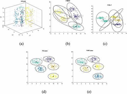
in Table 6. However proposed method F-MT-Lasso discard non-informative feature $x_3$ and as a results, it provided us with best average accuracy (AR = 1.00). The details of discarded feature through FG-Lasso and F-MT-Lasso against different values of $\lambda$are shown in Table 7. When we increase the value of $\lambda$to 50, we observed that both Algorithms completely discarded irrelevant feature $x_3$ and the obtained results have been shown in Table 7. It is clearly seen that after discarding irrelevant feature $x_3$ our proposed algorithm shows best results, that is the advantage and novelty of our method.

Table 6. Comparison of F-MB-N, FCML-T, FG-Lasso with F-MT-Lasso based on reduced feature and average AR.

Original features	Average AR		No. of remaining features		Average AR
	F-MB-N	FCML-T	FG-Lasso	F-MT-Lasso	FG-Lasso	F-MT-Lasso
3	0.627	0.8025	2	2	0.980	1.00

Table 7. Feature reduction pattern based on $\lambda$ values.

$\lambda$	Feature reduction pattern through FG-Lasso			Feature reduction pattern through F-MT-Lasso
	$x_1$	$x_2$	$x_3$	$x_1$	$x_2$	$x_3$
10	-	-	${\hat{\mu }}_{13}=0$	-	-	-
20	-	-	${\hat{\mu }}_{23}=0$	-	-	${\hat{\mu }}_{33}={\hat{\mu }}_{43}={\hat{\mu }}_{53}=0$
30	-	-	${\hat{\mu }}_{33}={\hat{\mu }}_{34}={\hat{\mu }}_{35}=0$	-	-	${\hat{\mu }}_{23}=0$
50	-	-		-	-	${\hat{\mu }}_{13}=0$

Application in the Field of Biosciences

Variable selection and dealing with outliers/noisy points in biological studies are challenging and important task. Due to having outliers and irrelevant features/genes in biological data sets, estimated parameters would be biased, insufficient and inconsistent. In order to demonstrate the effectiveness and real applicability of proposed method F-MT-Lasso we applied it in the following five sets of biological real data; seeds, Pima Indian, prostate cancer, breast cancer and soil data set. Soil data set have been collected from Gilgit-Baltistan, Pakistan in collaboration with Karakoram International University GB, Pakistan. Comparisons of the proposed F-MT-Lasso algorithm with F-MB-N, FCML-T and FG-Lasso have also been made in the following.

Example 4.

In this example, we consider the real data set of seeds from (Das, 2014). This data set consists of 7 real-valued continuous attributes, namely; area, perimeter, compactness, length of kernel, width of kernel, asymmetry coefficient and length of kernel groove. This data set comprised of three different varieties of wheat and Samples were labeled by numbers: 1–70 first variety of wheat “Kama wheat variety,” 71–140 for the “Rosa wheat variety,” and 141–210 for the “Canadian wheat variety.” 70 elements each, randomly selected for the experiment. To collect this data set, high quality visualization of the internal kernel structure was detected using a soft x-ray technique. This sort of technology is very familiar and famous because it is nondestructive and considerably cheaper. When the proposed F-MT-Lasso algorithm is applied to the data set, F-MT-Lasso and FG-Lasso both methods identified that 6^th feature is irrelevant one among a total of seven features. When the $\lambda$ value is increased up to 162, according to FG-Lasso we get ${\hat{\mu }}_{16}={\hat{\mu }}_{26}={\hat{\mu }}_{36}=0$ and consider features six as irrelevant and removed it from further clustering. After discarding this irrelevant feature, the average accuracy rate with 30 different initializations, we obtain (AR = 0.859) from FG-Lasso, (AR = 0.593) from F-MB-N, and (AR = 0.628) using FCML-T. When we increase the value of $\lambda$ = 200 we observed that${\hat{\mu }}_{16}={\hat{\mu }}_{26}={\hat{\mu }}_{36}=0$. 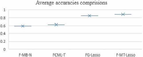Our proposed F-MT-Lasso algorithm discards feature six “asymmetry coefficient.” After discarding this feature from data, we execute our proposed F-MT-Lasso algorithm and get better average accuracy (AR = 0.891) with 30 different initializations. The comprision of each average accuracy rate has been shown is Table 8 and graphical comprision have been shown in Figure 5. This reveals that, the proposed F-MT-Lasso algorithm is significant and effective for relevant feature selection on the seeds data set.

Table 8. Comparison of F-MB-N, FCML-T, FG-Lasso with F-MT-Lasso based on reduced feature and average AR.

Original feature	Average AR		No. of remaining features		Average AR
	F-MB-N	FCML-T	FG-Lasso	F-MT-Lasso	FG-Lasso	F-MT-Lasso
7	0.593	0.628	6	6	0.859	0.891

Figure 5. Box and whisker plot of average accuracies from different methods.

Example 5.

In this example, we consider the real data set of Pima Indian (undefined). This data set consists of 8 predict variables and one response variable. The variables are named as pregnant, plasma, blood pressure (mm Hg), triceps skin fold thickness (mm), insulin (mu U/ml), body mass index (weight in kg/(height in m)^2), diabetes pedigree function, and age (years). While response variable is (1: diabetes, 0: not). The data set has two classes. Diabetes mellitus is very common and severe disease in many populations of the world including American Indian tribe and Indian. There are many risk factors of this disease and some well-known of those are parental diabetes, genetic markers, obesity, diet (Das, 2014). When the proposed FG-Lasso algorithm is applied to the Pima Indian diabetics data set, it identified that when we are increasing the value of $\lambda$ up to 50 using FG-Lasso, we get${\hat{\mu }}_{15}={\hat{\mu }}_{25}=0$, feature five “insulin” as irrelevant feature and after removing it, from further clustering we obtain (AR = 0.653) from FG-Lasso, (AR = 0.544) from F-MB-N, (AR = 0.5083) using FCML-T with the average of 30 different initializations. Our proposed method F-MT-Lasso also discards feature five “insulin” against the value of $\lambda$ = 150 and we get better average accuracy rate (AR = 0.720) with 30 different initializations. The comprision of each average accuracy rate has been shown is Table 9, while graphical comprision have been reflected in Figure 6. This confirms that, the proposed F-MT-Lasso algorithm is also significant for relevant feature selection on the Pima Indian data set.

Table 9. Comparison of F-MB-N, FCML-T, FG-Lasso with F-MT-Lasso based on reduced feature and average AR.

Original feature	Average AR		No. of remaining features		Average AR
	F-MB-N	FCML-T	FG-Lasso	F-MT-Lasso	FG-Lasso	F-MT-Lasso
8	0.544	0.628	7	7	0.653	0.720

Figure 6. Box and whisker plot of average accuracies from different methods.

Example 6

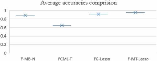
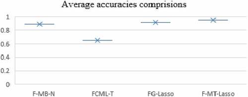
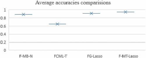
(Breast Cancer (UCI, 2019)) Breast cancer is one of the severe and commonest cause of death in women worldwide. It is frequently found in Australia/New-Zealand, United Kingdom, Sweden Finland, Denmark, Belgium (Highest rate), the Netherlands and France. According to the findings of World health organization, common causes of breast cancer are tobacco use, use of alcohol, dietary factors including lack of fruit and vegetable consumption, overweight,obesity, physical inactivity, chronic infections from helicobacter pylori, hepatitis B virus, hepatitis C virus and some type of human papilloma virus, environmental and occupational risks including ionizing and non-ionizing radiation (Bray et al., 2018; Siegel et al., 2019). In this example, we consider real data set regarding breast cancer that consist of eight features namely; clump thickness, uniformity of cell size, uniformity of cell shape, marginal adhesion, bare nuclei, bland chromatin, normal nucleoli, mitoses and one output variable class having 699 samples. When the proposed FG-Lasso algorithm is applied on this breast cancer data set, it has been observed that when we increase the value of $\lambda$ to 400, four features namely; clump thickness, marginal adhesion, normal nucleoli and mitoses are identified to be irrelevant features. So, after removing these four features from further clustering, we obtained (AR = 0.911) from FG-Lasso, (AR = 0.892) from F-MB-N, and (AR = 0.850) using FCML-T on the average, for 30 different initializations. On the other hand, our proposed method F-MT-Lasso discards only feature seven “normal nucleoli” against the same value of$\lambda$ = 400 and we get even more better average accuracy (AR = 0.962) with 30 different initializations. The comprision of each average accuracies are shown is Table 10 and graphical representation is shown in Figure 7. This reveals that, the proposed F-MT-Lasso algorithm is more significant and effective for relevant feature selection regarding breast cancer data set.

Table 10. Comparison of F-MT-Lasso with F-MB-N, FCML-T and FG-Lasso.

Original feature	Average AR		No. of remaining features		Average AR
	F-MB-N	FCML-T	FG-Lasso	F-MT-Lasso	FG-Lasso	F-MT-Lasso
8	0.892	0.842	4	7	0.911	0.962

Figure 7. Box and whisker plot of average accuracies from different methods.

Example 7

(Prostate cancer Saifi, 2018)) Prostate cancer is second major common type of cancer and fifth leading cause of death among men worldwide and occurs over the age of 70 years (Bray et al., 2018).This kind of cancer starts, when cells in the prostate gland start to grow out of control. The most leading countries in this domain are Australia, America, New Zealand, Norway, Sweden and Ireland (Bray et al., 2018). Here we consider a real prostate cancer data set consists of 100 patients of prostate cancer having eight features namely; radius, texture, perimeter, area, smoothness, compactness, symmetry, fractal dimension and one categorical parameter diagnosis results (benign tumors = 38 and malignant tumors = 68). When FG- Lasso algorithm is applied on the prostate cancer data set, this identified that when we are increasing the value of $\lambda$ up to 60, we observed the features like radius, texture, perimeter, and area as irrelevant features. After removing these irrelevant features, we obtain (AR = 0.617) from FG-Lasso, (AR = 0.517) from F-MB-N, and (AR = 0.635) using FCML-T after taking the average of 30 different initializations. When the proposed F-MT-Lasso algorithm is applied to the prostate cancer data set, it has been noticed that 4^th feature “area” became irrelevant feature against $\lambda$ = 78, and consequently has been discarded. Hence we found that after discardng it, we get better average accuracy rate (AR = 0.807) with 30 different initializations. The comprision of each average accuracy rate, are shown is Table 11 and graphical comparisons are shown in Figure 8. This shows that, the proposed F-MT-Lasso algorithm is more significant and effective for relevant feature selection of the prostate cancer data set.

Table 11. Comparison of F-MB-N, FCML-T, FG-Lasso with F-MT-Lasso based on reduced feature and average AR.

Original feature	Average AR		No. of remaining features		Average AR
	F-MB-N	FCML-T	FG-Lasso	F-MT-Lasso	FG-Lasso	F-MT-Lasso
8	0.517	0.762	4	7	0.617	0.807

Figure 8. Box and whisker plot of average accuracies from different methods.

A Real Application of Soil Data from the Region of Gilgit-Baltistan, Pakistan

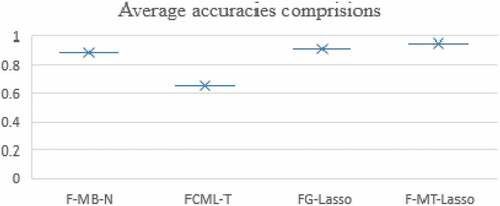
Finally, we apply our proposed F-MT-Lasso algorithm on real data set regarding soil which consists of thirty samples, ten samples in each cluster. The soil samples have randomly been taken from 0 to 15 cm depth with the help of small spade and hand trowel from three region (clusters) of Gilgit-Baltistan namely; Damote Sai (located in Hindukush range), Bunji (located in Himalya) and Jalalabad (located in Karakorum Range) with the collaboration of Karakoram international university Giglit-Baltistan. The purpose of taking samples from three different locations is to compare soil fertility status of regions. The samples have been dried and Sieved through a 2 mm sieve for further laboratory investigation. PH was measured through a pH probe by 1:1 (soil: water) suspension with OAKTON PC 700 meter (Mclean, 1983). EC was measured by 1:5 (Soil: water) with Milwaukec EC meter (SM 302) (Rayment and Higginson, 1992). Fertility status of soil NO3-N, P, K was determined by (AB- DTPA) extractable method (Jones, 2001). In all the samples of three regions, Nitrogen was detected as defecient or low range and our both methods FG-Gauss and F-MT-Lasso have suggested to discard the Nitrogen from soil data to improve the accuracy as shown in Table 12. Hussain et al., (2021) conducted research on soil fertility of two villages from lower Karakorum Range and the quantity of nitrogen was in range within marginal or medium range from both orchard and agricultural land. Whereas Babar et al. (2004) stated/reported the deficiency of nitrogen (0.08% only) in the soil of Gilgit region.

Table 12. Comparison of F-MB-N, FCML-T, FG-Lasso with F-MT-Lasso based on reduced feature and average AR.

Original feature	Average AR		No. of remaining features		Average AR
	F-MB-N	FCML-T	FG-Lasso	F-MT-Lasso	FG-Lasso	F-MT-Lasso
5	0.889	0.652	4	4	0.913	0.949

In the following we show scatter plots for all possible combinations of soil parameters in Figure 9 while graphical comprision have shown in Figure 10.

Figure 9. Scatter plots for all possible combinations of PH, EC, N, P and K.

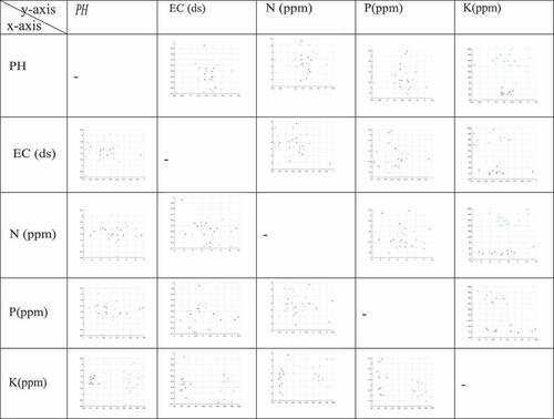
Figure 10. Box and whisker plot of average accuracies from different methods.

Conclusion

In model-based clustering many proposed methods are based on EM algorithm to overcome its sensitivity and initialization issues. However, these methods treat data points with feature (variable) components with equal importance, and so it cannot distinguish the irrelevant feature components. In most of the cases, there exist some irrelevant features and outliers/noisy points in a data set that adversely affect the performance of clustering algorithms. To identify and discard those irrelevant features or to handle the problems due to those outliers/noisy points, multivariate t-distribution is more efficient and effective than multivariate normal distribution due to its heavily. It is therefore we proposed a fuzzy model-based t-clustering schema using mixture of t-distribution with an $L_1$regularization for the better identification and selection of significant features and to improve the performance of algorithm against the sparsity exists in the data.

We have applied our proposed F-MT-Lasso algorithm on simulatd data sets as well as real data sets including seeds, pima, prostrate cancer, breast cancer and soil data data to show its effectivenss and usefulness.It has been seen from comparative analysis that the proposed F-MT-Lasso algorithm is a robust choice and provides better results with higher accuracy rates as compared to the existing methods for variouse larger values of threshold$\lambda$. However, our question is, which value of the threshold $\lambda$ would be the optimal value for better feature selection in the F-MT-Lasso algorithm? That is, to find a good estimate for the threshold parameter $\lambda$ is very important and would be our further topic in our future research.

Disclosure statement

We have no conflicts of interest to disclose.

References

- Abbasi, A., and M. Younis. 2007. A survey on clustering algorithms for wireless sensor networks. Computer Communications 30 (14–15):2826–492. doi:10.1016/j.comcom.2007.05.024.
- Agrawal, R., J. Gehrke, D. Gunopulos, and P. Raghavan. 2005. Automatic subspace clustering of high dimensional data for data mining applications. Data Mining and Knowledge Discovery 11 (1):5–33. doi:10.1007/s10618-005-1396-1.
- Babar, K., R. A. Khattak, and A. Hakeem. 2004. Physico-chemical characteristics and fertility status of Gilgit soils. Journal of Agricultural Research 42 (3–4):305–12.
- Banfield, J. D., and A. E. Raftery. 1993. Model-based Gaussian and non-Gaussian clustering. Biometrics 49 (3):803–21. doi:10.2307/2532201.
- Biernacki, C., and J. Jacques. 2013. A generative model for rank data based on insertion sort algorithm. Computational Statistics & Data Analysis 58:162–76. doi:10.1016/j.csda.2012.08.008.
- Bray, F., J. Ferlay, I. Soerjomataram, R. L. Siegel, L. A. Torre, and A. Jemal. 2018. Global cancer statistics 2018: GLOBOCAN estimates of incidence and mortality worldwide for 36 cancers in 185 countries. CA: A Cancer Journal for Clinicians 68 (6):394–424. doi:10.3322/caac.21492.
- Chuang, K. S., H. L. Tzeng, S. Chen, et al. 2006. Fuzzy c-means clustering with spatial information for image segmentation. Computerized Medical Imaging and Graphics. 30(1):9–15. doi:10.1016/j.compmedimag.2005.10.001.
- Das, R. N. 2014. Determinants of diabetes mellitus in the pima indian mothers and Indian medical students. The Open Diabetes Journal 7 (1):5–13. doi:10.2174/1876524601407010005.
- Dempster, A. P., N. M. Laird, and D. B. Rubin. 1977. Maximum likelihood from incomplete data via the EM algorithm. Journal of the Royal Statistical Society, Series B (Methodological) 39 (1):1–22. doi:https://doi.org/10.1111/j.2517-6161.1977.tb01600.x.
- Fraley, C., and A. E. Raftery. 2002. Model-based clustering, discriminant analysis, and density estimation. doi:10.1198/016214502760047131.
- Garibaldi, U., D. Costantini, S. Donadio, et al. 2006. Herding and clustering in economics: The Yule-Zipf-Simon model. Computational Economics. 27(1):115–34. doi:10.1007/s10614-005-9018-y.
- Gogebakan, M. 2021. A novel approach for Gaussian mixture model clustering based on soft computing method. IEEE Access 9:159987–60003. doi:10.1109/ACCESS.2021.3130066.
- Gogebakan, M., and H. Erol. 2018. A new semi-supervised classification method based on mixture model clustering for classification of multispectral data. Journal of the Indian Society of Remote Sensing 46 (8):1323–31. doi:10.1007/s12524-018-0808-9.
- Gogebakan, M., and E. Hamza. 2019. Mixture model clustering using variable data segmentation and model selection: A case study of genetic algorithm.Mathematics letters. Mathematics Letters 5 (2):23–32. doi:10.11648/j.ml.20190502.12.
- Hussain, A., H. Ali, F. Begum, A. Hussain, M. Khan, Y. Guan, J. Zhou, S. Din, and K. Hussain. 2021. Mapping of soil properties under different land uses in lesser karakoram range, Pakistan. Polish Journal of Environmental Studies 30 (2):1181–89. doi:10.15244/pjoes/122443.
- Jain, A. K., and C. R. 1988. Dubes: Algorithms for clustering data. New Jersey: Prentice Hall.
- Jones, J. B. 2001. Laboratory guide for conducting soil tests and plant analysis (No. BOOK). CRC press.
- Kadim, T., and C. Wirnhardt. 2012. Neural network-based clustering for agriculture management. EURASIP Journal on Advances in Signal Processing 2012 (1):1–13. doi:10.1186/1687-6180-2012-200.
- Lee, G., and C. Scott. 2012. EM algorithms for multivariate Gaussian mixture models with truncated and censored data. Computational Statistics & Data Analysis 56 (9):2816–29. doi:https://doi.org/10.1016/j.csda.2012.03.003.
- Lo, K., and R. Gottardo. 2012. Flexible mixture modeling via the multivariate t distribution with the box-cox transformation: An alternative to the skew-t distribution. Statistics and Omputing 22 (1):33–52. doi:10.1007/s11222-010-9204-1.
- McLachlan, G. J., and K. E. Basford. 1988. Mixture models: Inference and applications to clustering. vol. 38 New York: M. Dekker.
- McLean, E. O. 1983. Soil pH and lime requirement. Methods of soil analysis: Part 2 chemical and microbiological properties. 9:199–224.
- Mcnicholas, P. D. 2016. Model-based clustering. Journal of Classification 33 (3):331–73. doi:10.1007/s00357-016-9211-9.
- Melnykov, V., and I. Melnykov. 2012. Initializing the em algorithm in Gaussian mixture models with an unknown number of components. Computational Statistics & Data Analysis 56 (6):1381–95. doi:https://doi.org/10.1016/j.csda.2011.11.002.
- Pan, W., and X. Shen. 2007. Penalized model-based clustering with application to variable selection. Journal of Machine Learning Research 8 (5).
- Rasool, A., X. Tangfu, F. Farooqi, et al. 2016. Arsenic and heavy metal contaminations in the tube well water of Punjab, Pakistan and risk assessment: A case study. Ecological engineering 95:90–100. doi:10.1016/j.ecoleng.2016.06.034.
- Rayment, G. E., and F. R. Higginson. 1992. Australian laboratory handbook of soil and water chemical methods. Inkata Press Pty Ltd.
- Saifi, S. Prostate cancer dataset. https://www.kaggle.com/sajidsaifi/prostate-cancer
- Siegel, R. L., K. D. Miller, and A. Jemal. 2019. Cancer statistics, 2019. CA: A Cancer Journal for Clinicians 69 (1):7–34. doi:https://doi.org/10.3322/caac.21551.
- Tibshirani, R. 1996. Regression shrinkage and selection via the lasso. Journal of the Royal Statistical Society, Series B (Methodological) 58 (1):267–88. doi:10.1111/j.2517-6161.1996.tb02080.x.
- UCI Machine Learning Repository. 2019. World health statistics. Geneva. https://archive.ics.uci.edu/ml/index.php
- Xie, B., W. Pan, and X. Shen. 2007. Variable selection in penalized model-based clustering via regularization on grouped parameters. Biometrics 64 (3):921–30. doi:10.1111/j.1541-0420.2007.00955.x.
- Yang, M. S., and W. Ali. 2019. Fuzzy Gaussian Lasso clustering with application to cancer data. Mathematical Biosciences and Engineering 17 (1):250–65. doi:10.3934/mbe.2020014.
- Yang, M. S., Y. C. T. And, and Y. C. Lin. 2014. Robust fuzzy classification maximum likelihood clustering with multivariate t-distributions. International Journal of Fuzzy Systems 16:566–76.
- Yang, M. S., S. J. Chang-Chien, and Y. Nataliani. 2019. Unsupervised fuzzy model-based Gaussian clustering. Information Sciences 481:1–23. doi:10.1016/j.ins.2018.12.059.
- Yang, M. S., C. Y. Lai, and C. Y. Lin. 2012. A robust em clustering algorithm for Gaussian mixture models. Pattern recognition 45 (11):3950–61. doi:10.1016/j.patcog.2012.04.031.
- Zadeh, L. A. 1965. Fuzzy sets. Information and Control 8 (3):338–53. doi:https://doi.org/10.1016/S0019-9958(65)90241-X.