Paddy Yield Prediction in Tamilnadu Delta Region Using MLR-LSTM Model

ABSTRACT

Crop yield forecasting has been well studied in recent decades and is significant in protecting food security. Crop growth is a complex phenomenon that depends on various factors. Machine learning and deep learning trends have emerged as important innovations in this field. We propose to utilize crop, weather, and soil data from agricultural datasets to evaluate yield prediction behavior. Paddy being a staple food crop in India is chosen for this research. In this paper, we propose hybrid architecture for paddy yield prediction, namely, MLR-LSTM, which combines Multiple Linear Regression and Long Short-Term Memory to utilize their complementary nature. The results are compared with traditional machine learning methods such as Support vector machine, Long short-term memory and Random forest method. Evaluation metrics such as Coefficient of Determination (R²), Root Mean Square Error (RMSE), Mean Absolute Error (MAE), Mean Square Error (MSE), F1 score, Recall, and Precision are used to evaluate the hybrid method and traditional models. The results obtained from the proposed hybrid method indicates that the hybrid model delivers better R², RMSE, MAE, MSE values of 0.93, 0.1549, 0.199, and 0.024 respectively.

Introduction

Agriculture and allied sectors are the major contributors to Indian economy. For 2020–2021, agriculture and allied sectors contributed 20.2% of Gross Value Addition in our economy (Ministry of Agriculture & Farmers Welfare report., 2022). Rice is an important crop in India and iscultivated in places where there is abundant water supply. India is the second largest rice producer after China. Indian states majorly producing rice include West Bengal, Andhra Pradesh, Punjab, Tamil Nadu and Uttar Pradesh. India produced around 130.29 million tonnes in 2021–2022 as per reports by Department of Agriculture, India (Directorate of Economics and Statistics report., 2021–2022). Precision agriculture helps farmers to making decision for entire crop cultivation activities like irrigation, fertilizer application, seed selection, and harvesting. Nowadays, crop yield prediction has become a difficult task due to erratic weather changes and introduction of varieties of hybrid seeds. Current farming methods are completely different from our traditional farming. Rice farming in the region is thus monitored on a yearly basis as a result of official initiatives to assess rice-growing area and forecast rice production (Chen et al. 2011; Chou, Lei, and Chen 2006). The crop yield estimation or prediction depends on multiple factors like soil properties, weather, varieties of crop, genotype, and fertilizer usage. There were different types of crop simulating model used to develop the predictive model and estimated crop yields were reasonably accurate (van Klompenburg, Kassahun, and Catal 2020; Xu et al. 2019). Machine learning techniques and deep learning methods are crescively used to investigate non-linear relationships between a group of predictor variables and a target variable. They are frequently used for yield prediction.

In this study, the proposed MLR-LSTM algorithm is utilized to develop a prediction model for crop yield estimation and the integrated predictive model’s result is compared with Support vector machine, Long short-term memory and Random forest algorithms. This paper discusses the following objectives: first to build a predictive model to estimate the accurate yield prediction using MLR-LSTM hybrid technique on agricultural dataset collected from Joint Director of Agriculture Office in Thanjavur District; secondly to the yield prediction from the proposed hybrid model when compared with MLR, RF, SVM, and LSTM algorithms which shows that the hybrid MLR-LSTM model predicts efficiently and lastly, to compare the performance of these algorithms with proposed hybrid model using the Standard evaluation metrics.

The contents of this research article are sectionized as mentioned: Section 2 discusses the existing academic research works; Section 3 elaborates how the exact research work was executed; Section 4 contains the experimental results; and finally, Section 6 delivers the conclusion and future scopes.

Literature Review

Scholars are employing algorithms to provide accurate yield predictions based on the information available (Hund et al. 2018; Xing et al. 2018). The accuracy of the ML algorithms’ predictions and reservations is determined by the quality of input data, model prototyping, and relationship between the input and target variables in the collected datasets (Kotsiantis, Zaharakis, and Pintelas 2006; Kuo, Li, and Kifer 2018). Crop yield prediction is based on the input features like crop cycle, meteorological data, historical yield data as well as crop yield prediction algorithms (Ji et al. 2007; Jones et al. 2016). An improved yield forecast is being investigated by agricultural researchers, depends on meteorological data, agricultural data and improved yield prediction algorithms to increase the agricultural yield productivity (Basso, Cammarano, and Carfagna 2013). However standard dataset for agricultural research is limited. Dataset fluctuates according to the region, type of crop, season, and farming methods used (Drummond et al. 2003; Ji et al. 2007). Crop monitoring is currently one of the most difficult tasks in agricultural research, and it is critical for the success of the economy of any country (Prasad et al. 2006). Crop yield estimates have traditionally been based on field survey data provided by farmers during the crop growing season. However, they have challenges in terms of time consumption and labor costs over big areas (Anothai et al. 2013; Araya et al. 2015; Burke and Lobell 2017; Kuwata and Shibasaki 2016; Leroux et al. 2019). For a different method of yield estimation, Crop models are used to simulate the crop growth stages using various types of factors like genotype, meteorological data, soil properties, and field management practices. To establish the interaction between crop yield and observable variables, previous research concentrated on regression analysis or process-based models (Edreira and Otegui 2012; Fang et al. 2008). Existing machine learning techniques such as Random forest, Gaussian process regressor, and support vector machine regressor have already been used effectively to develop a relationship between crop productivity and input parameters because they can deal with the inbuilt non-linearity in the input data (Fieuzal, Sicre, and Baup 2017; Lobell et al. 2014). Deep learning algorithms also widely used for crop yield estimation and prediction. DNN algorithm trained with meteorological data (rainfall, temperature, perception, humidity, etc.) and soil properties were used to forecast crop yield (Ashapure et al. 2020). In existing work, they showed only yield forecast information for first stage of the crop cycle. In recent years, neural network study has been used for agriculture. Convolutional neural network also enhances the performance of the yield prediction (Cunha, Silva, and Netto 2018; Kamilaris and Prenafeta-Boldu 2018; Kamilaris, Kartakoullis, and Prenafeta-Boldú 2017; Lokers et al. 2016). Crop models use remote sensing as well as spatial information. The crop model employs remote sensing to give geographical inputs, and the research suggests that using a crop model and remote sensing together may identify management zones and sources of yield variability (Basso et al. 2001). For tomato crop yield estimation in existing work, images are used to predict the yield in early stages using tree ensemble method (Lillo-Saavedra 2022). Remote sensing data collected from MODIS is used to estimating yield for soybean crop using CNN-LSTM integrated model. Weather data, crop growth data, historical yield of soybean data, MODIS Land Surface Temperature and Surface reflectance factors are used to estimate yield in the integrated deep learning model (Sun 2019). Another one integrated model CNN-DNN developed to predict yield using publicly available dataset such as weather and soil data features for this study and compared with other deep learning algorithms (Oikonomidis, Catal, and Kassahun 2022). Based on the above-mentioned references, to improve precision with evaluation metrics for agricultural yield prediction, a more accurate and adequate method is required. Lack of prediction accuracy is one of the biggest problems with statistical methods, especially in environments with complicated data sets from several data sources. The study solves the problem of accurately predicting the future yield prediction with incomplete data.

Based on above existing works, the proposed research focuses on the below objectives:

• Study the paddy crop yield data from a high potential and a real-time location.

• Estimate the crop yield prediction by utilizing machine learning and deep learning technique.

• Propose a hybrid model for crop yield prediction.

• To study the model using evaluation metrics such as coefficient of determination (R²), Root mean square error (RMSE), mean square error (MSE) and mean absolute error (MAE), F1Score, Precision, Recall.

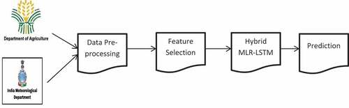
• Evaluate the performance of proposed model and other techniques based on evaluation metrics. Figure 1 shows the research overview of this paper.

  Figure 1. Overview of the Research.

  

Materials and Methods

Study Site

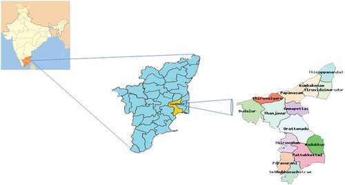
Thanjavur is one of the districts in Tamil Nadu. It is encompassed between 09’ 50’ and 11’ 25’ of the northern latitude and 78’ 45’ and 70 25’ of the Eastern longitude and covers 3396.57 square kilometers. Thanjavur district plays a major role in food grain production, thereby acquiring the name of “Rice bowl of Tamil Nadu.” In this district, rice is the principal crop. Traditionally, rice cultivation is done once or twice in a year. In this work, the entire district of Thanjavur is split into 14 blocks and their corresponding data affecting paddy yield is collected. The main reason for selecting this region is highest percentage of paddy yield is here. The soil type plays a crucial role in Thanjavur. The soil nature of Thanjavur district is made up of Cretaceous, Tertiary and Alluvial deposits. Figure 2 shows the study region in Tamil Nadu from where data is collected for the research.

Figure 2. Location area of study site Thanjavur District, Tamilnadu.

Dataset

The datasets used for this research are collected from Indian Meteorological Department, Chennai, and Joint Director of Agriculture Office, Kattuthottam, Thanjavur. Joint Director of Agriculture Office provided seven years of soil, weather and other crops growth factors data for the 14 blocks. The dataset here is limited as it is pertaining to paddy yield research in detail. Seven years of agricultural data along with climate data are used in this paper. The two different datasets (agriculture and climate) are combined to form a single dataset. The agricultural data contains harvesting area, pH range, water irrigation area, fertilizer details. The climate dataset contains rainfall, maximum and minimum temperature, and wind speed. There are in total 3461 instances of data features including rainfall (mm), maximum temperature (℃), minimum temperature (℃), Windspeed (km/h), soil reaction (pH range), and field (planting area) are documented from 2014 to 2021. Soil reaction is an indication of the acidity or alkalinity of soil. These data are used to do the yield prediction in the specified planting area known as fields. Table 1 shows description of inputs features in this study.

Table 1. Description of input features in dataset.

Parameters	Description
pH range	Soil Reaction
rainfall	Rainfall
maxtemp	Maximum Temperature
mintemp	Minimum Temperature
block	Field
Windspeed	Wind Speed

In the initial steps the dataset is pre-processed for the identification and understanding of features, removing missing values and robusting outliers. This is followed by the feature selection process. The quality of input data decides the quality of the output data. StandardScaler and RobustScaler function from Python library is used for data cleansing. In this dataset, each and every attribute has its own measurements. Dataset for the entire region of Thanjavur district was used for this study.

Data Processing

For better prediction, the dataset has been resized using the StandardScaler equation, followed by feature selection using SelectFromModel and finally removing the outliers using RobustScaler function. Most of the dataset contains missing values, redundant values, outliers, and error values. First, we removed missing values and outliers in the dataset.

StandardScaler: In this study, we used StandardScaler model in Python from sklearn.preprocessing package. The irrelevant and redundant input features deceive the model performance in a wrong way. The missing values are replaced with zero value in the dataset. In the dataset, all features do not contribute for yield prediction. Upon studying the entire dataset, first we get to know which feature is contributing more for creating the most efficient predictive model. Then we normalized the dataset using StandardScaler method. The process of normalization is scaling individuals to have unit norm. This technique is used to measure the similarity of the two samples using a quadratic form, such as the dot-product. Since all the datasets do not have same range of units or values, thus, we had to determine independent and dependent variables in the dataset. The removal of the mean and scaling to unit variance was necessary for standardization.

SelectFromModel: In Python Sklearn SelectFromModel was used to select the most relevant feature based on which consist of input parameter having feature importance value greater than or equal to specified threshold value. It helps to remove the irrelevant features from the dataset. In the selection process features are selected based on the weight, max_features() is used to set the number of maximum features select from the dataset. If we set none in the max_features() function, all features are kept in the dataset. The feature selection is only based on max_features() and threshold value.

RobustScaler: RobustScaler() function is used to remove the outliers in the dataset. This function is used to remove the median and scale the data in the range between 1^st and 3^rd quartile (default range is 25%−75%). The range is called interquartile range. RobustScaler uses the interquartile range so it is robust the outliers. Later, transform method median and interquartile range are applied into the new data. If outliers are present in the dataset, the median and interquartile range outperform the sample mean and variance. The formula used to calculate the interquartile range is as follows:

(1) $\frac{x_i-Q_1\left(x\right)}{Q_3\left(x\right)-Q_1\left(x\right)}$(1)

After data normalization, feature selection technique is utilized to select most contributing feature in the available dataset. Most relevant input features for the target variable is selected for developing an efficient predictive model. In the current dataset, there are 25 input features, out of which only a few features contribute to the proposed prediction model. Feature selection is done on the basis of its relevance for the current simulation scenario. For feature selection process, SelectFromModel from the scikit-learn library in Python is used. After all these processes are completed, the input features are fed into the proposed model using machine learning and deep learning technique.

Methodology

Multiple Linear Regression:

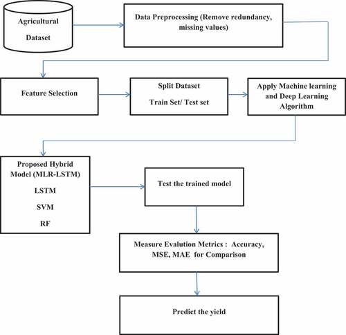
Figure 3 above shows the proposed framework for this research. Multiple linear regression (MLR) is the usual statistical method used for yield prediction. This method is chosen as there are multiple input features available in our dataset. Several academicians have used MLR to predict different crop yields. In MLR, Y, the dependent variable, depicts paddy yield and is in linear relation with multiple independent variables such as area of production, rainfall, temperature, and season indicated by x₁, x₂, x₃ … .x_n. The MLR equation can be written as,

(2) $\mathrm{Y}={\mathrm{a}}_0+{\mathrm{a}}_1{\mathrm{x}}_1+{\mathrm{a}}_2{\mathrm{x}}_2+{\mathrm{a}}_3{\mathrm{x}}_3+\dots \dots ..+{\mathrm{a}}_{\mathrm{n}}{\mathrm{x}}_{\mathrm{n}}$(2)

Figure 3. Proposed Framework of MLR-LSTM.

Here, a₀, a₁, a₂, a₃ … a_n are unknown parameters. a₀ is the bias and a₁, a₂, a₃ … a_n are coefficient of independent variables. Training the samples allows for the estimation of these parameters. In this work, previous yield temperature, rainfall, and area are taken as an independent feature used in MLR and yield is depicted as a dependent feature. This method is suitable for predicting linear relationship between dependent and independent variables. It is suitable for short-term dataset with not much feature variations. It is not suitable for a wide range of factors affecting yield prediction.

Multiple Linear Regression Framework.

Long Short-Term Memory:

Long Short-Term Memory network is usually denoted by LSTM, and it is a special type of Recurrent Neural Network. It was developed specifically for addressing the overall RNN’s issue of long-term dependence. It has been extensively applied in a variety of fields such as yield prediction, stock prediction, machine translation, and speech recognition. This method is useful to accommodate long-term data with varying data patterns. It is suited for executing non-linear data models. This method is also faster when compared to the traditional linear regression solution. Each RNN has a repeated neural network module in chain form. Input gate, Forget gate, and Output gate are primarily included. Figure 4 shows the LSTM framework.

Figure 4. The structure of LSTM network.

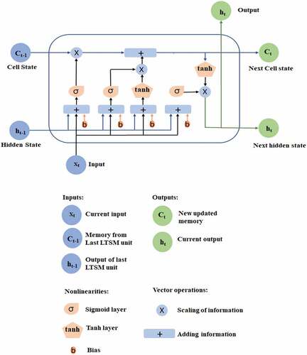
Forget Gate:

(3) $Z_{\mathrm{t}}=\delta (E_{\mathrm{f}}.[h_{t-1},x_{\mathrm{t}}]+b_{\mathrm{f}})$(3)

Throughout, the current input is the output of previous process. The outcome of the sigmoid function is multiplied by the cell state through the sigmoid function. The sigmoid function result outcome is between 0 and 1. If the result is near 0 it represents that the information is forgotten, while if the result is near 1 it represents that it keeps the information. Z_t is current output value, E_f is the weight of current output, b_f is a biased of current output, and h_t−1 is the output value of the previous layer.

Input Gate:

(4) $J_{\mathrm{t}}=\delta (E_{\mathrm{i}}.[h_{t-1},x_{\mathrm{t}}]+b_{\mathrm{i}})$(4)

(5) ${\tilde{C}}_{\mathrm{t}}=tanh(E_{\mathrm{B}}.[h_{t-1},x_{\mathrm{t}}]+b_{\mathrm{B}})$(5)

Input gate is to update the status of the old unit. Prior forget layer identifies what information is old or forgot and is being used by the input gate. This gate consists of two functions, namely sigmoid and tanh. These determine the information to be added to the state. Sigmoid layer is the first layer and identifies the values to be updated. Tanh layer identifies the additional information to be added to the existing state.

The above Forget gate and Input gate are the two-step process of removing unnecessary information and adding new required information which is shown in the following equation:

(6) $C_t=Z_t\ast C_{t-1}+J_t\ast \widetilde{C_t}$(6)

Output Gate:

(7) $P_{\mathrm{t}}=\delta (W_{\mathrm{p}}.[h_{t-1},x_{\mathrm{t}}]+b_{\mathrm{p}})$(7)

(8) $h_{\mathrm{t}}=P_t\ast tanh(C_{\mathrm{t}})$(8)

Output gate provides the value of next hidden state. It contains information of previous inputs. The value of current state and the preceding hidden state are received by the third sigmoid function. Following that, the tanh function is applied to the new cell state that results from the cell state. These two results are multiplied one by one. The network determines which information the hidden state should contain based on the final value. This hidden state is used for prediction. The forget gate contains the information that we get from the previous step. What significant information from the current step can be added is decided by the input gate and output gate that conclude the next hidden state. Table 2shows the definition of variables used in LSTM method.

Table 2. Definition of Variables for LSTM Components.

Variables	Definition
xt	Input Variable (Intercept and Coefficient values from MLR)
ht	Hidden Variable at the current time step t
ht-1	Hidden variable from the previous time step t-1
Ct	Cell state variable at the current time step t
Ct-1	Cell state variable from the previous time step t-1
Ot	Output Variable

Hybrid MLR-LSTM:

Multiple Linear Regression (MLR) is a statistical approach in machine learning. It is used to analyze the linear relationship between independent variables and dependent variable. It is suitable for short-term dataset. For short-term dataset, MLR provides faster execution and accurate results. This method can be easily implemented for datasets with similar patterns and simple in nature. The major drawback in MLR for yield prediction is that for large dataset this algorithm does not perform efficiently. This method is not scalable for a large dataset. It is challenging when it is established in a large dataset. Computation time is increased for larger data. When we integrate data from various sources, datasets become complex and exhibit different data patterns. Considering the above, MLR prediction accuracy is not efficient for paddy yield forecasting model. The following factors are used to predict the yield:

Forecasting yield = Linear relationship factors + Non-linear factors + fluctuated yield differences

Multiple linear regression model is used for analyzing the correlation between independent variable and dependent variable. In this method a number of independent variables are processed with the dependent variables. Six parameters are used in this evaluation; dataset contains time series data such as rainfall, minimum temperature, maximum temperature, and wind speed. MLR method helps to analyze the correlation between these input features, and it is used to choose which data feature is fit for the linear model. The bias, residual, and coefficient for the input features are calculated using this model. It is essential to develop a hybrid model framework for yield prediction combining machine learning and deep learning techniques due to the nonlinearity and complexity of the features. LSTM method is used commonly for long-term and multi-pattern and non-linear datasets. The proposed hybrid method efficiently utilizes both the benefits of MLR-LSTM in this way, producing significantly improved outcomes. For yield prediction, MLR helps to find the correlation of one feature with another feature. In existing works, the researchers who implemented MLR for yield prediction report low prediction value. The highly correlated input features are causing the low-level prediction. For a large set of time-series data, it took more time for prediction and collinearity problem will occur when highly correlated data features in the dataset. The calculated residual from MLR is input for next stage of LSTM network.

(9) $Residual\hspace{0.17em}\left(e\right)\hspace{0.17em}=\hspace{0.17em}Actual\hspace{0.17em}\left(t\right)\hspace{0.17em}-\hspace{0.17em}Predicted\hspace{0.17em}\left(t_{\mathit{1}}\right)$(9)

Long short-term memory is a time-series algorithm in deep learning. This method is used to process sequence of time-series data and long-term deficiency is rectified. The structure of the LSTM, which specializes in processing sequential data, both retains significant information and predicts the sequential data. In extended sequence training, LSTM is primarily used to address gradient disappearance and explosion. The residual calculated from MLR model forms the input for LSTM network through the input gate. The current time step output forms the hidden layer in the next time step process. This method trains the model for time series data. Forget gate removes unwanted and repeated data sets. MLR’s output data, when fed into LSTM, provides more accurate results with fewer iterations and run time. As LSTM is a closed loop algorithm, the process repeats itself till the current output result extracted matches the previous time step. This trained model gives efficient prediction results compared with other techniques. The proposed hybrid MLR-LSTM method is efficient than the traditional machine learning algorithms. This is discussed in detail in the result section.

To overcome this problem, MLR-LSTM algorithms are used to integrated in this proposed work. This integrated framework helps to reduce the error rate of the prediction model. Also, for large data the processing time will be reduced. The proposed hybrid model when compared with existing models, error rate, and processing time decreases when used with a large dataset.

Following Steps Performed for Hybrid MLR-LSTM

 Step 1: Collect data from agricultural and meteorological department

Step 2: Do Data pre-processing for collected data

Step 3: After normalization, split the dataset into training and testing set

Step 4: Apply Multiple linear regression algorithm to the training dataset

 4.1: Calculate the intercept and coefficient of each variables and residual using equation (2)(2) $\mathrm{Y}={\mathrm{a}}_0+{\mathrm{a}}_1{\mathrm{x}}_1+{\mathrm{a}}_2{\mathrm{x}}_2+{\mathrm{a}}_3{\mathrm{x}}_3+\dots \dots ..+{\mathrm{a}}_{\mathrm{n}}{\mathrm{x}}_{\mathrm{n}}$(2) , equation (9)(9) $Residual\hspace{0.17em}\left(e\right)\hspace{0.17em}=\hspace{0.17em}Actual\hspace{0.17em}\left(t\right)\hspace{0.17em}-\hspace{0.17em}Predicted\hspace{0.17em}\left(t_{\mathit{1}}\right)$(9)

Step 5: Use Long short-term memory model

 5.1: Initialise hidden layer as 1

 5.2: Initialise number of epochs as 500

 5.3: Initialise learning rate 0.1

Step 6: Initialize the lstm input layer bias, residual and weights with step 4.1 value

 Calculate Z_t , $\tilde{B}$_t, and J_t using equation (3)(3) $Z_{\mathrm{t}}=\delta (E_{\mathrm{f}}.[h_{t-1},x_{\mathrm{t}}]+b_{\mathrm{f}})$(3) ,equation (4)(4) $J_{\mathrm{t}}=\delta (E_{\mathrm{i}}.[h_{t-1},x_{\mathrm{t}}]+b_{\mathrm{i}})$(4) , and equation (5)(5) ${\tilde{C}}_{\mathrm{t}}=tanh(E_{\mathrm{B}}.[h_{t-1},x_{\mathrm{t}}]+b_{\mathrm{B}})$(5)

 Update cell state C_t using equation (6)(6) $C_t=Z_t\ast C_{t-1}+J_t\ast \widetilde{C_t}$(6)

 Calculate P_t and h_t using equation (7)(7) $P_{\mathrm{t}}=\delta (W_{\mathrm{p}}.[h_{t-1},x_{\mathrm{t}}]+b_{\mathrm{p}})$(7) equation (8)(8) $h_{\mathrm{t}}=P_t\ast tanh(C_{\mathrm{t}})$(8)

Step 7: Calculate error rate using evaluation metrics

Step 8: Feed forward process proceed until the error is minimized

Step 9: Display the result

End Model

Evaluation Metrics

In this study, different evaluation metrics are applied to evaluate the predictive model. We used the following evaluation metrics: coefficient of determination (R²), mean square error (MSE), and mean absolute error (MAE). F1 score, precision, and recall values are calculated in this work. The following equations in Table 3 provides the formulae for evaluation metrics used in this study.

Table 3. Evaluation metrics used in this study.

$R^2=1-\frac{\sum {\left(y_i-\hat{y}\right)}^2}{\sum {\left(y_i-\bar{y}\right)}^2}$	$MSE=\frac{1}{N}\sum _{i=1}^N(y_i-\hat{y}{)}^2$
$MAE=\frac{1}{n}\sum _{i=1}^n\left|{\hat{y}}_i-y_i\right|$	$RMSE=\sqrt{MSE}=\sqrt{\frac{1}{N}\sum _{i=1}^N{\left(y_i-\hat{y}\right)}^2}$
$Precision=\frac{TP}{TP+FP}$	$Accuracy=\frac{TN+TP}{TN+FP+TP+FN}$
$Recall=\frac{TP}{TP+FN}$	$F1Score=2\ast \frac{Recall\ast Precision}{Recall+Precision}$

Mean square error determines the average of the squares of error. Mean square error value calculates average squared between predicted and actual values. Mean absolute error denotes the absolute difference between the predicted value and the actual value. Coefficient of determination denotes proportion of the variation in the dependent variable that is predictable from the independent variables. It ranges between 0 and 1. All the equations are performed using Python language in Google colab.

Result and Discussion

In this section, statistical and proposed hybrid model are demonstrated in a virtual platform. The statistical analysis acquires various input features: rainfall, temperature, wind speed, soil type, previous yield, and pH range. The model with the higher correlation and smaller error scale will be regarded as the most accurate method for predicting crop yield. First phase represents the result of the statistical model, namely Multiple Linear Regression. For the second phase, the input layer bias and weights of the LSTM were initialized using the MLR intercept and coefficients.

Various research showed that machine learning techniques could forecast paddy yield. However, improving prediction accuracy is necessary for a reliable agricultural yield. Performance evaluation metrics such as R², MSE, RMSE, and MAE are applied to evaluate the performance of the proposed hybrid model and other machine learning and deep learning algorithm such as RF, SVM, and LSTM for crop yield prediction. The aforementioned formulae are used to evaluate each metric. The accuracy of the algorithms under evaluation is then examined using the metrics between the predicted and actual crop yield.

The comparative analysis between different algorithms using evaluation metrics, namely R², MSE, RMSE, and MAE. Accuracy of the system is characterized by higher R² (closer to unity) and lower RMSE, MAE, MSE. This study shows that the proposed hybrid model performed well against the machine learning and deep learning algorithms. The coefficient of determination metric of hybrid model achieved a better value of about 0.934. When compared with other algorithms the proposed method gives better outcomes.

Additionally, the RMSE metric of hybrid model shows a lower value of about 0.1549. The accuracy result of the crop yield is compared with other methods. Likewise, the metrics of MSE, MAE show the lower value for hybrid model about 0.024, 0.199, respectively, which are compared with other algorithms such as RF, SVM, and LSTM. Table 4 and Figure 5 shows the evaluation metrics comparison results in a tabular and graphical format respectively. Also Table 5 and Figure 6 shows superior performance of the proposed hybrid-model agains standard machine learning algorithms. All these results demonstrate the precision of the paddy yield prediction for Thanjavur zone in Tamil Nadu. Datasets used are collected from the official meteorological and agricultural department. Comparing these inferences, the proposed hybrid model gives superior results with other algorithms such as RF, SVM, and LSTM using evaluation metrics. The prediction accuracy of the proposed model is compared with other methods from literature. The evaluation metrics values are compared with existing methodologies. The absolute yield of the study site location is compared with the other previous works. Thanjavur has achieved the highest yield in Tamilnadu due to ideal parameters of the district such as mean temperature, higher rainfall, and pH range. Also, a variety of alluvial soil that is suited for paddy farming can be found in Thanjavur paddy cultivation areas. The hybrid model predicted values almost match Thanjavur’s absolute yield, but with varying precision depending on how well each algorithm performs. It is already stated that the hybrid model performance shows better outcome than other machine learning and deep learning models.

Figure 5. Comparative analysis (i) R², (ii) MSE, (iii) MAE, (iv) RMSE between proposed and other models.

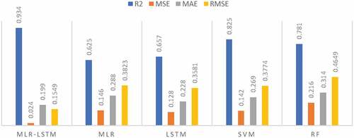
Figure 6. Comparative analysis (i) Accuracy, (ii) Precision, (iii) Recall, (iv) F1_Score between proposed and other models.

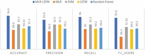
Table 4. Comparative analysis (i) R², (ii) MSE, (iii) MAE, (iv) RMSE between proposed and other models.

Methods	R^2	MSE	MAE	RMSE
MLR-LSTM	0.934	0.024	0.199	0.1549
MLR	0.625	0.146	0.288	0.3823
LSTM	0.657	0.128	0.228	0.3581
SVM	0.825	0.142	0.269	0.3774
RF	0.781	0.216	0.314	0.4649

Table 5. Comparative analysis (i) F1Score, (ii) Recall, (iii) Precision, (iv) Accuracy between proposed and other models.

	MLR-LSTM	MLR	SVM	LSTM	Random Forest
Accuracy	96.6	89.6	92.4	90.34	91.4
Precision	94.6	88.9	92.3	92.3	90.2
Recall	96	90	92.3	90.2	90.6
F1_Score	95.6	86.2	91.02	89.9	90.3

Conclusion

Statistical and machine learning algorithms are used to predict agricultural yield. To achieve agricultural yield prediction with improved efficiency, the deep learning techniques and machine learning algorithms like RF, SVM, and LSTM and our proposed hybrid model are taken into consideration for evaluation. Performance metrics of the various models are examined to determine the accuracy of the various algorithms. With the observed outcomes, the following conclusions are made:

1. Based on the outcomes of evaluation measures, the proposed hybrid model achieved higher yield forecast accuracy than other algorithms.

2. The proposed hybrid model predicted the crop yield more precisely compared with RF, SVM, and LSTM algorithms.

3. Coefficient of determination (R²), mean square error (MSE), root mean square error (RMSE), and mean absolute error (MAE) performance metrics of the proposed hybrid model showed a result 0.934, 0.024, 0.1549, and 0.199 respectively.

4. The R² metrics of the proposed improved to compare with the other existing from the literature reports.

5. When Thanjavur’s absolute yield is compared to other districts of Tamilnadu, it is discovered that Thanjavur has the highest yield, and that this yield can be achieved using the proposed hybrid prediction model with more accuracy.

6. The analysis also reached the conclusion that the study site (Thanjavur) has the rainfall, temperature, and pH level that paddy farmers need to grow their crops to their highest potential output.

7. The proposed hybrid model reduces the risk factor for crop yield due to its higher performance metrics.

In future, the proposed method is applied to other delta region and also calculate the method processing time and will be add more metrics and input parameters for next work. Future studies should concentrate on establishing the effects of various factors on agricultural yield prediction and achieving multimodal data fusion.

Disclosure statement

No potential conflict of interest was reported by the authors.

References

- Anothai, J., C. M. T. Soler, A. Green, T. J. Trout, and G. Hoogenboom. 2013. Evaluation of two evapotranspiration approaches simulated with the CSM-CERES-Maize model under different irrigation strategies and the impact on maize growth, development and soil moisture content for semi-arid conditions. Agricultural and Forest Meteorology 176:64–583. doi:10.1016/j.agrformet.2013.03.001.
- Araya, A., G. Hoogenboom, E. Luedeling, K. M. Hadgu, I. Kisekka, and L. G. Martorano. 2015. Assessment of maize growth and yield using crop models under present and future climate in southwestern Ethiopia. Agricultural and Forest Meteorology 214-215:252–65. doi:10.1016/j.agrformet.2015.08.259.
- Ashapure, A., J. Jung, A. Chang, S. Oh, J. Yeom, M. Maeda, A. Maeda, N. Dube, J. Landivar, S. Hague, et al. 2020. Developing a machine learning based cotton yield estimation framework using multi-temporal UAS data. Isprs Journal of Photogrammetry and Remote Sensing 169:180–94. doi:10.1016/j.isprsjprs.2020.09.015.
- Basso, B., D. Cammarano, and E. Carfagna, 2013. Review of crop yield forecasting methods and early warning systems. In Proceedings of the First Meeting of the Scientific Advisory Committee of the Global Strategy to Improve Agricultural and Rural Statistics (pp. 15–31). 10.1017/CBO9781107415324.004.
- Basso, B., J. T. Ritchie, F. J. Pierce, R. P. Braga, and J. W. Jones. 2001. Spatial validation of crop models for precision agriculture. Agricultural systems 68 (2):97–112. doi:https://doi.org/10.1016/S0308-521X(00)00063-9.
- Burke, M., and D. B. Lobell. 2017. Satellite-based assessment of yield variation and its determinants in smallholder African systems. PNAS Agricultural Sciences 114 (9):2189–94. doi:10.1073/pnas.1616919114.
- Chen, C. -F., S. -W. Huang, N. -T. Son, and L. -Y. Chang. 2011. Mapping double-cropped irrigated rice fields in Taiwan using time-series satellite pour I ‘observation De La terre data. Journal of Applied Remote Sensing 5 (1):053528. doi:10.1117/1.3595276.
- Chou, T. Y., T. C. Lei, and H. H. Chen. 2006. “Application of boosting to improve image image classification accuracy in rice parcel with decision tree”. Paper presented at the ACRS.
- Cunha, R. L. F., B. Silva, and M. A. S. Netto, 2018. A scalable machine learning system for preseason agriculture yield forecast. In proceeding of IEEE 14th International Conference on e-Science (e-Science) . 423–30. 10.1109/eScience.2018.00131.
- Drummond, S. T., K. A. Sudduth, A. Joshi, S. J. Birrell, and N. R. Kitchen. 2003. Statistical and neural methods for site-specific yield prediction. Trans American Society of Agricultural and Biological Engineers 46 (1):5–14. doi:10.13031/2013.12541.
- Edreira, J. I. R., and M. E. Otegui. 2012. Heat stress in temperate and tropical maize hybrids: Differences in crop growth, biomass partitioning and reserves use. Field Crops Research 130:87–98. doi:10.1016/j.fcr.2012.02.009.
- Fang, H., S. Liang, G. Hoogenboom, J. Teasdale, and M. Cavigelli. 2008. Corn yield estimation through assimilation of remotely sensed data into the CSM-CERES-Maize model. International Journal of Remote Sensing 29 (10):3011–32. doi:10.1080/01431160701408386.
- Fieuzal, R., C. M. Sicre, and F. Baup. 2017. Estimation of corn yield using multi-temporal optical and radar satellite data and artificial neural networks. International Journal of Applied Earth Observation and Geoinformation 57:14–23. doi:10.1016/j.jag.2016.12.011.
- Government of India, Department of Agriculture & Farmers Welfare Ministry of Agriculture & Farmers Welfare. 2022. Annual Report 2021-2022. Government of India, Krishi Bhawan, New Delhi. Accessed February 08, 2023. https://agricoop.nic.in/Documents/annual-report-2021-22.pdf
- Hund, L., B. Schroeder, K. Rumsey, and G. Huerta. 2018. Distinguishing between model- and data-driven inferences for high reliability statistical predictions. Reliability Engineering & System Safety 180:201–10. doi:10.1016/j.ress.2018.07.017.
- Ji, B., Y. Sun, S. Yang, and J. Wan. 2007. Artificial neural networks for rice yield prediction in mountainous regions. The Journal of Agricultural Science 145 (3):249–61. doi:10.1017/S0021859606006691.
- Jones, J. W., J. M. Antle, B. Basso, K. J. Boote, R. T. Conant, I. Foster, H. Charles, J. Godfray, M. Herrero, R. E. Howitt, et al. 2016. Brief history of agricultural systems modeling. Agricultural systems 155:240–54. doi:10.1016/j.agsy.2016.05.014.
- Kamilaris, A., A. Kartakoullis, and F. X. Prenafeta-Boldú. 2017. A review on the practice of big data analysis in agriculture. Computers and Electronics in Agriculture 143:23–37. doi:10.1016/j.compag.2017.09.037.
- Kamilaris, A., and F. X. Prenafeta-Boldu. 2018. Deep learning in agriculture: A survey. Computers and Electronics in Agriculture 147:70–90. doi:10.1016/j.compag.2018.02.016.
- Kotsiantis, S. B., I. D. Zaharakis, and P. E. Pintelas. 2006. Machine learning: A review of classification and combining techniques. Artificial Intelligence Review 26:159–90. doi:10.1007/s10462-007-9052-3.
- Kuo, Y., H. Z. Li, and D. Kifer, 2018. Detecting outliers in data with correlated measures. In proceeding of 2018 ACM Conference on Information and Knowledge Management (CIKM’18), pp. 22–26. 10.1145/3269206.3271798.
- Kuwata, K., and R. Shibasaki. 2016. Estimating corn yield in the United States with MODIS EVI and machine learning methods. ISPRS Annals of the Photogrammetry, Remote Sensing and Spatial Information Sciences 8 (3):131–36. doi:10.5194/isprs-annals-III-8-131-2016.
- Leroux, L., M. Castets, C. Baron, M. J. Escorihuela, A. B´egu´e, and S. Lo. 2019. Maize yield estimation in West Africa from crop process-induced combinations of multi-domain remote sensing indices. European Journal of Agronomy 108:11–26. doi:10.1016/j.eja.2019.04.007.
- Lillo-Saavedra, M. 2022. Early estimation of tomato yield by decision tree ensembles. Agriculture (MDPI) 12 (10):1655. doi:10.3390/agriculture12101655.
- Lobell, D. B., M. J. Roberts, W. Schlenker, N. Braun, B. B. Little, R. M. Rejesus, and G. L. Hammer. 2014. Greater sensitivity to drought accompanies maize yield increase in the U.S. Midwest Science 344 (6183):516–19. doi:10.1126/science.1251423.
- Lokers, R., R. Knapen, S. Janssen, Y. V. Randen, and J. Jansen. 2016. Analysis of big data technologies for use in agro-environmental science. Environmental Modelling & Software 84:494–504. doi:10.1016/j.envsoft.2016.07.017.
- Oikonomidis, A., C. Catal, and A. Kassahun. 2022. Hybrid deep learning-based models for crop yield prediction. Applied Artificial Intelligence 36 (1):2031822. doi:10.1080/08839514.2022.2031823.
- Prasad, A. K., L. Chai, R. P. Singh, and M. Kafatos. 2006. Crop yield estimation model for Iowa using remote sensing and surface parameters. International Journal of Applied Earth Observation and Geoinformation 8 (1):26–33. doi:10.1016/j.jag.2005.06.002.
- Sun, J. 2019. County-level soybean yield prediction using deep CNN-LSTM model. Sensors (MDPI) 19 (20):4363. doi:10.3390/s19204363.
- van Klompenburg, T., A. Kassahun, and C. Catal. 2020. Crop yield prediction using machine learning: A systematic literature review. Computers and Electronics in Agriculture 177:105709. doi:10.1016/j.compag.2020.105709.
- Xing, L., L. Li, J. Gong, C. Ren, J. Liu, and H. Chen. 2018. Daily soil temperatures predictions for various climates in United-States using data-driven model. Energy 160:430–40. doi:10.1016/j.energy.2018.07.004.
- Xu, X., P. Gao, X. Zhu, W. Guo, J. Ding, C. Li, M. Zhu, and X. Wu. 2019. Design of an integrated climatic assessment indicator (ICAI) for wheat production: A case study in Jiangsu Province, China. Ecological indicators 101:943–53. doi:10.1016/j.ecolind.2019.01.059ecolind.2019.01.059,https://pib.gov.in/PressReleasePage.aspx?PRID=1741942