Neural Networks And Ensemble Based Architectures To Automatic Musical Harmonization: A Performance Comparison

ABSTRACT

Harmony can be defined in a musical way as art that combines several musical notes reproduced simultaneously to create sounds that are coherent to human ears and serve as accompaniment and filling. However, working out harmony is not a simple task. It requires knowledge, experience, and an intense study of music theory, which takes time to reach good skills. Thus, systems capable of automatically harmonizing melodies are beneficial for experienced and novice musicians. In this paper, a comparative study between distinct architectures and ensembles of Artificial Neural Networks was proposed to solve the problem of musical harmonization, seeking consistent results with rules of music theory: Multilayer Perceptron (MLP), Radial Basis Function network (RBF), Echo State Network (ESN), Extreme Learning Machines (ELM), and Long Short-Term Memory (LSTM). For this, a processed and defined melody with symbolic musical data serves as input to the system, having been trained from a musical database that contains melody and harmony. The output is the chord sequence to be applied to the melody. The results were analyzed with quantitative measures and the ability to melody adaptation. The performances were favorable to the MLP, which could generate harmonies according to the objectives.

Introduction

When a set of musical notes is played simultaneously, a sound called chord is formed. When several chords are put in order, there is harmony. Naturally, such harmonies are designed to accompany musical melodies, which bring meaning, proportion, and symmetry to a song (Roig-Francolí 2010). Therefore, harmony, among other definitions, can be a way to choose chords that correctly complement a musical line.

The harmonic choices for a given melody are limited, although several options can fit the exact musical moment. However, like any form of art, the harmonization of a given melody requires time, experience, and musical study, especially concerning harmony theory (Koops, Pedro, and de Haas 2013).

Understanding the harmonization task as an analytical process, researching its constitution, and finding a way to automate it represents a valuable contribution to the study of music, artificial intelligence, and Musical Information Retrieval (MIR) (Koops, Pedro, and de Haas 2013).

Several attempts to solve the problem of automatic music harmonization exist in the literature, often using evolutionary methods, such as with Genetic Algorithms (GAs) (Nakashima et al. 2010; Wiggins, Papadopoulos, and Phon-Amnuaisuk 1998), statistics (Chuan 2011) or with rule-based systems (Ebcioğlu 1988; Koops, Pedro, and de Haas 2013).

Neural Networks have also been used. In Lim and Lee (2017), the authors applied Bidirectional Long Short-Term Memory (BLSTM) networks, trained in symbolic data of actual song harmonies, reaching 50% accuracy. In Rhyu et al. (2022), an architecture based on transformers was applied, with three proposed models; some of which showed the ability to learn about a song in its entirety with better-structured results than those obtained by applying LSTMs. Similarly, Yeh et al. (2020) conducted a comparative study of five harmonizing models, two of which involve recurrent ANNs, with results evaluated from objective and subjective metrics. Other works, such as Dong et al. (2017); Huang and Wu (2016); Liu and Yang (2018), seek to use similar methodologies, however, with a different objective, which is the whole music generation, including melody and even the arrangement.

In this paper, different architectures and ensembles of Artificial Neural Networks (ANNs) were applied to solve the problem of harmonizing music, motivated by understanding the behavior of this specific Artificial Intelligence method. Their performance were compared for the following algorithms: Multilayer Perceptron (MLP), Radial Basis Function network (RBF), Echo State Network (ESN), Extreme Learning Machines (ELM), and Long Short-Term Memory (LSTM). Using a database of symbolically represented songs containing melodies and chords, the ANNs were trained and later became able to generate new harmonies. Statistical and performance measures were calculated on the results of each model to describe the production quality, making it possible to compare them quantitatively and choose the best one. The results met the objectives, reaching consistent and reasonable performance levels, presenting as novelty a comparison focused only in using ANNs.

This paper is divided into sections of which: Sections 2 and 3 briefly describe musical harmony theory and establish the applied methodology, respectively. Results are exposed and discussed in Section 4, of which conclusions are drawn in Section 5.

Musical Harmony Theory

According to Schoenberg (1978), harmony is the study of sounds played simultaneously and their relationship between architectural, melodic, and rhythmic values, as well as their meaning and relative strength to each other (Schoenberg 1978). The study of harmony establishes essential rules and concepts, some of which are presented below, according to Western Tonal Music.

The construction of chords can be commonly done using triads, which are three musical notes played simultaneously, usually consisting of notes overlapping in intervals of thirds. Depending on the type of these intervals, the chords can be named as major, minor, augmented, or diminished (Terefenko 2014).

The term diatonic chords is used to refer to the group of chords that can be played on a given note scale. In it are inserted the chords that constitute a functional relationship with each other. For example, the chords used in the key of C major are C major (or maj), D minor (or min), E min, F maj, G maj, A min, and B min flatted fifth (or diminished) (Roig-Francolí 2010).

In harmony terms, function is understood as the characteristic of a chord, having its value concerning the others. The tone is defined by essential functions traditionally called tonic, dominant, and subdominant, respectively, each represented by a chord. For the other chords present in the diatonic chords, their functions are inherited from the main functions, called secondary functions, and these chords can be named as relatives (Terefenko 2014).

Respecting these functions, the normal movement of the chords within the song is established as (Roig-Francolí 2010):

• The dominant function is commonly preceded by the tonic, giving the resolution of the dissonance (in the tonic);

• The subdominant function has greater freedom, but its sense of movement usually leads to the dominant;

• The tonic function is usually applied at the beginning or at the end of a song or musical phrase, giving the idea of completion.

Exemplifying using the C major diatonic chords: G maj chord has a dominant function and B diminished is its relative; F maj is subdominant, and its relative is D min; and for the tonic function, there is C maj, with A min and E min being their relative.

Functional harmony aims to study the functioning of these functions and establish rules and concepts for their correct use within the music. By understanding the functions, it is possible to harmonize songs coherently. Also, rules that, when respected, indicate the quality of the work (Roig-Francolí 2010; Terefenko 2014).

Proposed Method for Automatic Musical Harmonization

The proposed method for this work is illustrated in Figure 1 and can be described in some steps: a database containing both melody and harmony of several songs in symbolic format is standardized in terms of tonality, note duration and chord types. Then, input notes and output chords are encoded into numeric vectors. These vectors are used for training ANNs models, which will be able to generate conditioned harmonies by the melodies at the entrance, a chord by measure¹ (Roig-Francolí 2010). These ANNs models then will be used to create ensembles. The resulting harmonies will be evaluated quantitatively compared to the original harmonies.

Figure 1. Block diagram showing the proposed methodology, step by step, described in order.

The following will discuss how musical data processing is done, the description of the ANNs and ensembles used, and the measures used for quantitative evaluation.

Data Processing

To carry out the training of the ANNs, data are needed. We use the CSV Leadsheet Database (Lim, Rhyu, and Lee 2017). It contains songs of rock, pop, country, jazz, folk, R&B, children’s songs, etc., in CSV format, all in major key. Each row of the CSV is a musical event, an occurrence of a new note or chord. Every song file has the following features:

• Time: the song’s time signature at the moment;

• Measure: the musical measure where the event is located;

• Key fifths and key mode: details the song tonality;

• Chord root and chord type: what chord is being played, root note and type (major, minor, dominant, among others);

• Note root and note octave: what note is being played and the octave it is located;

• Note duration: how long the note should be executed, considering the whole note with a value equal to 16.

More processing phases are necessary to use this data for the training of ANNs. First, the songs need to be standardized, and then, information needs to be encoded to be understood by the models.

Standardization is an important step because the songs in the database have a great diversity of tonalities, rhythms and harmonies, as is their nature. Analyzing music considering all this diversity would be a complex and possibly impractical task, therefore standardization takes place at the following levels:

• Tonality: to keep information consistent, the songs are all transposed into a common tone. In this case, all the songs were transposed to C major tone, which gives higher confidence about which notes to expect and defines a common set of diatonic chords;

• Note duration: in that database, the duration of each note follows a numerical pattern independent of the metric or time signature² (Roig-Francolí 2010). However, the sum of notes durations of a measure will also be different for different time signatures, which requires normalization. Therefore, the length of each note can be multiplied by the inverse of the song’s time signature (Costa et al. 2022). In this way, all measures will have the same total duration;

• Chord types: one must consider the vast amount of chords that the chaining of musical notes can form as a problem. To simplify the possible system responses, only major and minor triads were considered, resulting in 24 chord classes.

Following these steps, there is a standardized tone, rhythm, and harmony database. The encoding of both notes and chords is done using the one-hot method. In this sense, a vector ${\mathbf{n}}_{\mathrm{n}\mathrm{o}\mathrm{t}\mathrm{e}}$ is used to represent a musical note. This vector contains 12 elements representing each note of the chromatic scale plus one position for pauses. Thus, the note D$\mathrm{\#}$ could be written as (1):

(1) ${\mathbf{n}}_{\mathrm{D}\mathrm{\#}}=[000100000000].$(1)

Likewise, the representation of a chord takes a vector ${\mathbf{c}}_{\mathrm{c}\mathrm{h}\mathrm{o}\mathrm{r}\mathrm{d}}$ of 24 positions, 12 for major chords and 12 for minor chords, interspersed with each other, for example, C maj, C minor, C$\mathrm{\#}$ maj, C$\mathrm{\#}$ minor, D maj, and so on. In that way, D maj chord is represented as (2):

(2) ${\mathbf{c}}_{\mathrm{D}\mathrm{m}\mathrm{a}\mathrm{j}}=[000010000000000000000000].$(2)

Considering that the analysis takes place by musical measure, a chord and a variable number of notes and rests are used for one measure. For a given measure, consider that three musical notes are played in sequence: D, F, and C. The encoding of each note would result in the following matrix ${\mathbf{N}}_{\mathrm{N}\mathrm{P}\mathrm{M}\times 12}$, where NPM stands for Notes Per Measure and 12 is the size of ${\mathbf{n}}_{\mathrm{n}\mathrm{o}\mathrm{t}\mathrm{e}}$ (3):

(3) ${\mathbf{N}}_{3\times 12}=\left[\begin{array}{cccccccccccc}0& 0& 1& 0& 0& 0& 0& 0& 0& 0& 0& 0\\ 0& 0& 0& 0& 0& 1& 0& 0& 0& 0& 0& 0\\ 1& 0& 0& 0& 0& 0& 0& 0& 0& 0& 0& 0\end{array}\right]$(3)

To simplify this matrix into a single vector, the lines are added, which leads to the sum vector $\mathbf{s}$ (4):

(4) $\mathbf{s}=[101001000000].$(4)

Thus, for each measure, there is ${\mathbf{c}}_{\mathrm{c}\mathrm{h}\mathrm{o}\mathrm{r}\mathrm{d}}$ for the chord and $\mathbf{s}$ representing the notes.

Artificial Neural Networks

For this work, the performance of five different architectures of ANNs is compared. They are described below.

Multilayer Perceptron (MLP)

Its main characteristic is the existence of at least one intermediate (hidden) layer of neurons between the input and output layers of the network, being conventional the use of only one or even two hidden layer (Haykin 2008). It is a versatile model with wide application in areas such as universal functions approximation, time series forecasting, systems optimization, and pattern recognition (Kachba et al. 2020; Siqueira and Luna 2019). In an MLP, neurons from different layers are densely connected, but there is no connection between those of the same layer. The training takes place in a supervised manner using the backpropagation algorithm (Haykin 2008). This paper employed two MLPs: one and two hidden layers.

Radial Basis Function Networks (RBF)

Local learning networks like the RBF usually consist of three layers, the input layer consisting only of source nodes to connect the data to the network. The hidden layer does not calculate weights with the input layer and uses nonlinear radial-based activation functions like the Gaussian. The training of this layer is performed using clustering algorithms, such as the K-Means. Finally, the output layer presents weights between the hidden layer; being these weights adjusted using backpropagation or the Moore-Penrose Pseudo-Inverse (MPPI) operation (Haykin 2008). It is possible to use linear or nonlinear functions as activation functions of the output neurons (Siqueira and Luna 2019). The sequential use of nonlinear and linear transformations takes advantage of the fact that, for a classification problem, increasing the information space dimension gives a greater probability of finding a linear separation (Haykin 2008). This finding is a desirable attribute since, for the problem of this paper, the number of classes is relatively large.

Extreme Learning Machine (ELM)

The great advantage of the ELMs when compared to the traditional MLP is its fast learning process, and good generalization performance with the universal approximation capability (de Souza Tadano, Siqueira, and Alves 2016; Siqueira et al. 2012b). It is a feedfoward architecture and only one hidden layer, in which the weights are not adjusted; that is, it has fixed parameters. Thus, during the training phase, there is no manipulation of the cost function, which is summarized to find the best output layer weights. This task can be accomplished with a linear combiner, which can be done by using MPPI operation (Huang, Zhu, and Siew 2006; Siqueira et al. 2020). Furthermore, the multitude of musical note arrangements for a given chord requires a model with good generalization capabilities, making it enjoyable to use this network model (Tadano et al. 2021).

Echo State Network (ESN)

Unlike the previous ones, this is a Recurrent Neural Network (RNN). That is, present feedback loops of information, presenting an intrinsic memory capability (Ribeiro, Reynoso-Meza, and Siqueira 2020). A three-layer structure is also considered, with a source input layer and a linear combiner based on the MPPI operation as output. The hidden layer is referred to as dynamic reservoir and contains sparsely interconnected neurons with fixed weights (Jaeger 2010). It has similarities with ELM since the learning process only modifies the weights for the output layer, being efficient due to the fast convergence (Siqueira et al. 2012a). The presence of memory can be attractive because the choice of chord sequences depends not only on the notes played in some measures but also on the context in which they are inserted, that is, on the notes and chords previously played in the song.

Long Short-Term Memory (LSTM)

As the ESN case, LSTM is a type of RNN with extended memory capacity. That is, compared to a conventional RNN, LSTM can “remember” information in arbitrary values of distance from the starting point, which is the advantage of LSTM (Hochreiter and Schmidhuber 1997). This network has a chain structure that contains four neural networks and different memory blocks called cells, where information is retained (Hochreiter and Schmidhuber 1996). Memory manipulation is done by three “gates” (Yao et al. 2015): Forget Gate, which removes useless information; Input Gate, which controls the addition of information; and Output Gate, responsible for extracting useful information from the current state of the cell and presenting it as network output. Its use can be justified similarly to the ESN, adding comparability between tests.

Ensembles

After the training phase, we can create ensembles of ANNs and compare their results. The ensemble is a combination methodology of multiple already trained models to improve the final system response (Wichard and Ogorzalek 2004). This combination is because different methods produce different behaviors with the same inputs. A model can present better responses for some input, while another works better for a different kind. A combination approach is then applied to generate the final ensemble output, for example, average, voting, or another neural network (Neto et al. 2021; Piotrowski Pawełand Baczyński et al. 2022).

There is still the necessity of simultaneously presenting diversity and having accurate predictions from each model. The purpose of an ensemble is to improve already existing good results. Ensembles have been used to solve many problems (Belotti et al. 2020; ?). This work tested three different ensembles: considering all ANNs, the best three, and the best two considering the error return.

Quantitative Evaluation

As this is a multiclassification problem, considering inputs and outputs as one-hot encoded vectors, the most indicated and commonly used training metric loss is the Categorical Cross-Entropy Loss, also called Softmax Loss (Gómez 2018).

To assess the efficiency of each model, classically, accuracy would be applied. However, as the database used in the training process is composed of actual songs, we can expect it to be unbalanced due to the musical nature of using some notes and chords more than others. Therefore, care must be taken when using accuracy, as it is a problematic measure when dealing with an unbalanced database because the impact of less represented but more critical examples is reduced compared to the majority class (Branco, Torgo, and Ribeiro 2015).

Other measures can be used to assess the quality of results, which take into account the issue of unbalance, such as Macro F1-score ($F_{1M}$) (Powers 2007), Matthews Correlation Coefficient (MCC) (Cramer 1962) and Cohen’s Kappa Coefficient ($\kappa$) (Cohen 1960).

Experimental Results

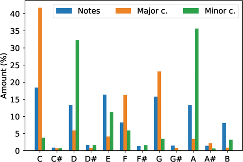
The results of the applied proposed methodology for automatic musical harmonization are described. In all, 2250 songs were standardized and filtered. For computational performance and availability reasons, only 20% of the total data was used, with 91,179 notes and 18,235 chords and measures, as only one chord per measure is being considered. Figure 2 shows the percentage of the total amount of notes and major and minor chords after the database processing phase.

Figure 2. Percentage of notes, major and minor chords present in 20% of the database, for each of the 12 possible notes considered in Western Tonal Music.

The following models were evaluated: one-layer MLP (MLP1), two-layers MLP (MLP2), RBF, ESN, LSTM, and ELM. From those, three ensemble models were also evaluated using voting as combination approach, considering all six networks (ENS6), only the top three (ENS3) and two (ENS2) best regarding loss results. To carry out the network training and testing stages, 60% of the data were separated for training, 20% for validation, and 20% for testing.

Tests were performed considering the variation in the number of neurons in the hidden layer, passing the values 64, 128, and 256. For the models that need training epochs (MLP1, MLP2, RBF and LSTM), the selected stopping criterion was a total number of epochs equal to 200, using Stochastic Gradient Descent with $\eta =0.001$ as the optimizer, saving the best weights when the minimum validation error value is reached for Categorical Cross-Entropy as a function of losses. ELM and ESN were implemented as described in Subsection 3.2.

To analyze the results, each model was run 30 times. In Table 1 it is possible to observe the average results of loss, accuracy, $F_{1M}$, MCC, and $\kappa$ of each model for the number of neurons that brought the best performance, considering the test set. Therefore, ENS3 is the ensemble of MLP1, MLP2, and RBF, and ESN2 is made of MLP1 and MLP2. On average, the models had a $F_{1M}$ of 13.88%, an MCC of 32.43%, and a $\kappa$ of 31.06%. As we are dealing with an unbalanced database, accuracy as an evaluation measure can bring wrong conclusions about the results, but for reasons of comparison and standard, they are also included.

Table 1. Average loss and accuracy, $F_{1M}$, MCC and $\kappa$ percentage for each model tested. Neurons are shown in parentheses.

Experiment	Loss	ACC (%)	F1%)	MCC (%)	$\kappa$ (%)
MLP1 (256)	1.7356	46.89	15.69	33.19	32.13
MLP2 (64)	1.7376	46.99	14.04	33.20	32.06
RBF (256)	1.7699	46.33	10.17	31.97	30.61
ELM (256)	2.1070	47.06	16.37	33.21	31.90
ESN (256)	2.1931	44.64	9.31	29.31	27.31
LSTM (64)	1.8485	45.65	15.59	32.12	31.02
ENS6	2.0076	46.94	15.55	33.08	31.56
ENS3	1.7743	47.02	14.04	33.05	31.63
ENS2	1.7676	46.75	14.19	32.71	31.29

Friedman Friedman (1937) test was applied to the results for the 30 runs of each model regarding the loss in the test set. The p-values achieved were equal to $9.52\times {10}^{-44}$. Therefore, it is possible to assume that there are significant changes in the results for different architectures.

Considering the metrics, loss, $F_{1M}$, MCC, and $\kappa$ each model was checked an overall performance (Table 2) for each result, using the Borda count method. The first place was awarded 8 points, the second 7, until the last place received 1 point. For loss, the first place is the smallest value, and for all other metrics, the first place is the biggest value.

Table 2. Overall ranking using Borda count method considering different metrics and algorithm results.

Experiment	Loss	F1	MCC	$\kappa$	Total
MLP1	9	8	7	9	33
MLP2	8	4	8	8	28
ELM	2	9	9	7	27
ENS2	7	5	4	4	20
ENS6	3	6	6	5	20
ENS3	5	3	5	6	19
LSTM	4	7	3	3	17
RBF	6	2	2	2	12
ESN	1	1	1	1	4

Next, a more in-depth analysis of the response of each model is made. An example of melody and its model-generated harmony, as well as the original harmony, is shown in Figure 3 for the first eight measures of the song America by Stephen Sondheim and Leonard Bernstein, composed for the musical West Side Story from 1957. The song has a rhythmic construction of hemiola,³ a repetitive melody, and simple harmony (Miller 2006). An interesting point is between measures 5 and 7, where there is a rapid modulation⁴ (Roig-Francolí 2010) passing through the key of C minor, making this an appropriate example to perceive the ability of generalization for the chosen models.

Figure 3. Melody of the song America represented with (a) score notation and (b) original and generated harmony by each evaluated model.

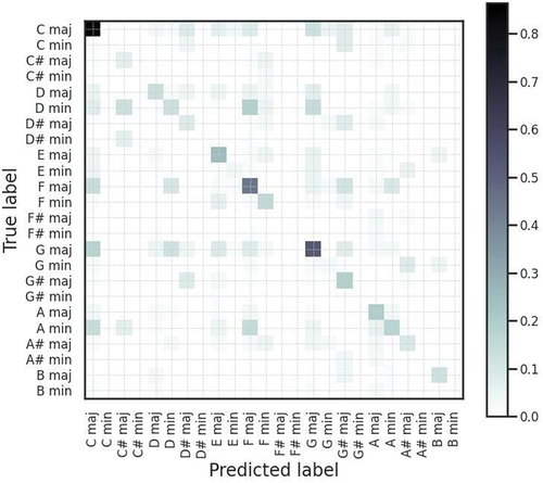
An efficient way to analyze the response of the selected model (MLP1) is to look at its confusion matrix, which can be seen in Figure 4.

Figure 4. Normalized confusion matrix for classifying chords using the MLP1 model.

Further discussion about the presented results are made in the following Subsection 4.1.

Discussion

It is interesting to note in Figure 2 a more significant presence of notes C, D, E, G, and A, corresponding to 77.03% of the total notes. These notes are part of a musical scale called “pentatonic,” widely used in styles like blues and rock, evidently present in several other styles due to its functionality.

The notes F and B appear in second place, completing the C major scale, as expected after the tonal transposition phase. Nevertheless, notes with accidents ($\mathrm{\#}$) are also present, demonstrating the plurality of the database used. Similarly, basic function chords (C maj, F maj, and G maj) and primary relatives (D min and A min) are the most substantial presence in the pieces of music, leading to the belief that the harmony employed must be relatively simple for most songs, although all types of chords exist in some proportion, for the 24 types considered. Furthermore, the fact that the database is unbalanced is still notorious.

Considering the results in Tables 1 and 2, in general, MLP1 obtained the best performance result, with the best loss and $\kappa$ and second-best $F_{1M}$. MLP2 and ELM almost tied for second, despite ELM’s loss being the second-worst of all models. In the sequence, the three ensembles, with ENS2 and ENS6 tied, and ENS3 with a difference of only one point. The fact that a singular model was able to return better results is relevant, even though the ensemble methods are the union of the best estimators.

Now, analyzing the harmonization shown in Figure 3, for the first four measures, all models responded with the same chords as the original harmony, probably because the melody notes are very indicative of the appropriate chord. For example, in measures 2 and 4, the notes together are the same that make up the F maj (F, A, and C) and G maj (G, B, and D) chords, respectively. The same goes for the last measure analyzed, where the notes are the same as the C maj chord (C, E, and G).

It is different when observing the interval from 5 to 7: RBF made the worst choices, proving to be unable to identify the modulation; ESN similarly, except for a possibly more appropriate choice for measure 5, that has the A$\mathrm{\#}$ note present; The LSTM chose the same chord as the original for measure 6, and the minor relative for measure 7, an interesting behavior, but a not-so-good choice for measure 5, as B may have only one note that correctly harmonize the measure (D$\mathrm{\#}$); MLPs, ELM and all ensembles made the same choices for measures 6 and 7, equal to the original, but it is clear that there was difficulty in finding a chord for measure 5. One reason for this could be that the original harmony uses a chord that is not considered, C min7 and only two notes are being played in this measure, A$\mathrm{\#}$ and D$\mathrm{\#}$. The most suitable choice would be D$\mathrm{\#}$ maj, since the notes in that measure are its root and fifth, respectively, the chosen one by MLP1, ELM, and all ensembles.

The previous analysis allows us to infer differences between the performance and interpretation of each model. In addition, based on the data presented, the one-layer MLP model is chosen as the most appropriate, with its best execution reaching a loss of 1.7356, and 15.90% $F_{1M}$, 33.00% MCC, and 31.84% $\kappa$. This $\kappa$ value allows us to state that this is a reasonable result (Artstein and Poesio 2008).

The formation of a diagonal line in the matrix of Figure 4 is slightly noticeable, a desirable characteristic since it means correct class assignments. This characteristic is most noticeable at specific points, as in the chords of C maj, F maj, and G maj, which are the main tonic functions. In addition, some columns of predicted classes stand out: C maj, F maj, and G maj. These columns lead us to understand that the model was able to comprehend the role that these chords play in musical harmony and can generalize the results, using them in a simplified way.

Conclusion

Different neural and ensemble models were proposed, tested, and evaluated for the task of automatic musical harmonization based on melodies.

The final harmonizing system was the MLP model with one hidden layer and 256 neurons, a model widely used in literature. It proved to be a reasonable nonlinear mapper in this field as well. The accuracy of the best model among 30 rounds reached 46.79%, a considerable result considering the results found in the literature for more complex models, and compared to a random guess. Keep in mind that 24 chord classes with uniform distribution would have a 4.17% chance of selection. The results generally show that the system has a simplifying capacity since harmony rules were not disregarded for the results generated.

For future work, we intend to explore models that can achieve higher classification accuracy values and use other means of quantifying the results to consider more rules of music theory, such as considering harmonic and relative functions. Another possibility is to interview listeners about the quality of the results, if they can differentiate if the system harmonized a piece of music or not, or ask music experts to evaluate the harmonizations, achieving a more subjective evaluation. Also, carry out a study on other ways of representing the input data since simplification in a sum vector sacrifices the order in which the notes are played and their duration, potentially compromising the results.

Acknowledgements

The authors thank the Brazilian agencies Coordination for the Improvement of Higher Education Personnel (CAPES) - Financing Code 001, Brazilian National Council for Scientific and Technological Development (CNPq), processes number 40558/2018-5, 315298/2020-0, and Araucaria Foundation, process number 51497, and Federal University of Technology - Parana (UTFPR) for their financial support.

Disclosure statement

No potential conflict of interest was reported by the author(s).

Correction Statement

This article has been republished with minor changes. These changes do not impact the academic content of the article.

Notes

1. Division of a piece of music into a time series.

2. Grouping of values with musical meaning, for rhythmic determination.

3. Alternating rhythm between binary and tertiary metrics.

4. Provisional character change of tone.

References

- Artstein, R., and M. Poesio. 2008. Inter-coder agreement for computational linguistics. Computational Linguistics 34 (4):555–859. dec. https://direct.mit.edu/coli/article/34/4/555-596/1999. Retrieved from.
- Belotti, J., H. Siqueira, L. Araujo, S. L. Stevan, P. S. de Mattos Neto, M. H. Marinho, J. F. L. de Oliveira, F. Usberti, M. D. A. Leone Filho, and A. Converti. (2020). Neural-based ensembles and unorganized machines to predict streamflow series from hydroelectric plants. Energies 13 (18):4769. doi:10.3390/en13184769.
- Branco, P., L. Torgo, and R. Ribeiro (2015, may). A survey of predictive modelling under imbalanced distributions. Retrieved from http://arxiv.org/abs/1505.01658
- Chuan, C. (2011). A comparison of statistical and rule-based models for style-specific harmonization. In International Society for Music Information Retrieval Conference, Miami, Florida, USA, (pp. 221–26).
- Cohen, J. 1960. A coefficient of agreement for nominal scales. Educational and Psychological Measurement 20 (1):37–46. apr. Retrieved from http://journals.sagepub.com/doi/10.1177/001316446002000104.
- Costa, L. F. P., A. Y. C. Ogoshi, M. S. R. Martins, and H. V. Siqueira (2022). Developing a measure image and applying to deep learning. In Music encoding conference. Halifax, CA: Music Encoding Initiative.
- Cramer, H. 1962. Mathematical methods of statistics. 1st ed. Bombay: Asia Publishing House.
- de Souza Tadano, Y., H. Siqueira, and T. Alves (2016). Unorganized machines to predict hospital admissions for respiratory diseases. In Latin american conference on computational intelligence, Cartagena, Colombia, (pp. 1–6).
- Dong, H. -W., W. -Y. Hsiao, L. -C. Yang, and Y. -H. Yang (2017). MuseGAN: Multi-track sequential generative adversarial networks for symbolic music generation and accompaniment. In AAAI conference on artificial intelligence, San Francisco, California, USA, (pp. 34–41).
- Ebcioğlu, K. 1988. An expert four-part harmonizing chorales. Computer Music Journal 12 (3):43–51. doi:10.2307/3680335.
- Friedman, M. 1937. The use of ranks to avoid the assumption of normality implicit in the analysis of variance. Journal of the American Statistical Association 32 (200):675–701. doi:10.1080/01621459.1937.10503522.
- Gómez, R. (2018). Understanding Categorical Cross-Entropy Loss, Binary Cross-Entropy Loss, Softmax Loss, Logistic Loss, Focal Loss and all those confusing names. Retrieved 2021-11-02, from https://gombru.github.io/2018/05/23/cross entropy loss/
- Haykin, S. 2008. Neural Networks and learning machines. 3rd ed. Hamilton, ON: Prentice Hall.
- Hochreiter, S., and J. Schmidhuber (1996). Lstm can solve hard long time lag problems. In Proceedings of the 9th international conference on neural information processing systems (p. 473–79). Cambridge, MA, USA: MIT Press.
- Hochreiter, S., and J. Schmidhuber. 1997, nov. Long short-term memory. ( Retrieved from) Neural Computation 9 (8):1735–80. doi: 10.1162/neco.1997.9.8.1735.
- Huang, A., and R. Wu. (2016). Deep learning for music. Deep Learning for Natural Language Processing. doi:10.48550/ARXIV.1606.04930.
- Huang, G. -B., Q. -Y. Zhu, and C. -K. Siew. 2006. Extreme learning machine: Theory and applications. Neurocomputing 70 (1–3):489–501. doi:10.1016/j.neucom.2005.12.126.
- Jaeger, H. (2010). The “echo state” approach to analysing and training recurrent neural networks – with an Erratum note (Tech. Rep. No. 148). GMD - German National Research Institute for Computer Science.
- Kachba, Y., D. Chiroli, J. Belotti, T. Alves, Y. de Souza Tadano, and H. Siqueira. 2020. Artificial neural networks to estimate the influence of vehicular emission variables on morbidity and mortality in the largest metropolis in south america. Sustainability 12 (7):2621. doi:10.3390/su12072621.
- Koops, H., M. Pedro, and W. de Haas (2013). A functional approach to automatic melody harmonisation. In Acm sigplan international conference on functional programming, Boston, Massachusetts, USA, (p. 47–58).
- Lim, H., and K. Lee (2017). Chord generation from symbolic melody using BLSTM networks. In International society for music information retrieval conference, Suzhou, China, (pp. 621–27).
- Lim, H., S. Rhyu, and K. Lee (2017). CSV Leadsheet Database. Retrieved 2019-06-08, from http://marg.snu.ac.kr/chordgeneration/
- Liu, H. -M., and Y. -H. Yang (2018). Lead sheet generation and arrangement by conditional generative adversarial network. In International conference on machine learning and applications, Paris, France, (pp. 722–27). IEEE.
- Miller, N. (2006). Heritage and Innovation of Harmony: A Study of West Side Story ( Unpublished doctoral dissertation). University of North Texas.
- Nakashima, S., Y. Imamura, S. Ogawa, and M. Fukumoto (2010). Generation of appropriate user chord development based on interactive genetic algorithm. In International conference on p2p, parallel, grid, cloud and internet computing, Fukuoka, Japan, (p. 450–53).
- Neto, P. S. D. M., P. R. A. Firmino, H. Siqueira, Y. D. S. Tadano, T. A. Alves, J. F. L. De Oliveira, M. H. D. N. Madeiro, and F. Madeiro. (2021). Neural-based ensembles for particulate matter forecasting. IEEE Access 9:14470–90. doi:10.1109/ACCESS.2021.3050437.
- Piotrowski Pawełand Baczyński, D., M. Gulczyński, T. Kopyt, and T. Gulczyński. 2022. Advanced ensemble methods using machine learning and deep learning for one-day-ahead forecasts of electric energy production in wind farms. Energies 15 (4):1252. doi:10.3390/en15041252.
- Powers, D. M. W. (2007). Evaluation: From precision, recall and F-measure to ROC, informedness, markedness and correlation (Tech. Rep). Adelaide: Flinders University. Retrieved from http://arxiv.org/abs/2010.16061
- Rhyu, S., H. Choi, S. Kim, and K. Lee. 2022. Translating melody to chord: Structured and flexible harmonization of melody with transformer. IEEE Access 10:28261–73. 02. doi: 10.1109/ACCESS.2022.3155467.
- Ribeiro, V., G. Reynoso-Meza, and H. Siqueira. 2020. Multi-objective ensembles of echo state networks and extreme learning machines for streamflow series forecasting. Engineering Applications of Artificial Intelligence 95:103910. doi:10.1016/j.engappai.2020.103910.
- Roig-Francolí, M. 2010. Harmony in Context. 2nd ed. Cincinnati, OH: McGraw-Hill.
- Schoenberg, A. 1978. Theory of Harmony. 1st ed. Berkeley, CA: University of California Press.
- Siqueira, H., L. Boccato, R. Attux, and C. Lyra Filho (2012a). Echo state networks for seasonal streamflow series forecasting. In International conference on intelligent data engineering and automated learning, Natal, Brazil, (pp. 226–36).
- Siqueira, H., L. Boccato, R. Attux, and C. Lyra Filho. 2012b. Echo state networks in seasonal streamflow series prediction. Learning and Nonlinear Models 10:181–91. doi:10.21528/LNLM-vol10-no3-art5.
- Siqueira, H., and I. Luna. 2019. Performance comparison of feedforward neural networks applied to streamflow series forecasting. Mathematics in Engineering Science and Aerospace 10 (1):41–53.
- Siqueira, H., M. Macedo, Y. D. S. Tadano, T. A. Alves, S. L. Stevan Jr, D. S. Oliveira Jr, M. H. N. Marinho, P. S. G. D. M. Neto, J. F. L. D. Oliveira, I. Luna, et al. 2020. … others. Energies 13 (16):4236. doi:10.3390/en13164236.
- Tadano, Y. S., S. Potgieter-Vermaak, Y. R. Kachba, D. M. Chiroli, L. Casacio, J. C. Santos-Silva, C. A. B. Moreira, V. Machado, T. A. Alves, H. Siqueira, et al. 2021. Dynamic model to predict the association between air quality, COVID-19 cases, and level of lockdown. Environmental Pollution 268:115920. doi:10.1016/j.envpol.2020.115920.
- Terefenko, D. 2014. Jazz theory: From basic to advanced study. 1st ed. Rochester, NY: Routledge.
- Wichard, J. D., and M. Ogorzalek (2004). Time series prediction with ensemble models. In International joint conference on neural networks, Shenzhen, China, (Vol. 2, pp. 1625–30). IEEE.
- Wiggins, G., G. Papadopoulos, and S. Phon-Amnuaisuk. 1998. Evolutionary methods for musical composition. International Journal of Computing Anticipatory Systems 2:10–14.
- Yao, K.N.A.I.N., T. Cohn, K. Vylomova, K. Duh, and C. Dyer (2015). Depth-gated LSTM. CoRR, abs/1508.03790 <publisher-name/>. Retrieved from http://arxiv.org/abs/1508.03790
- Yeh, Y. -C., W. -Y. Hsiao, S. Fukayama, T. Kitahara, B. Genchel, H. -M. Liu, H. -W. Dong, Y. Chen, T. Leong, and Y. -H. Yang (2020). Automatic melody harmonization with triad chords: A comparative study. arXiv. Retrieved from https://arxiv.org/abs/2001.02360