Interpretable SAM-kNN Regressor for Incremental Learning on High-Dimensional Data Streams

ABSTRACT

In many real-world scenarios, data are provided as a potentially infinite stream of samples that are subject to changes in the underlying data distribution, a phenomenon often referred to as concept drift. A specific facet of concept drift is feature drift, where the relevance of a feature to the problem at hand changes over time. High-dimensionality of the data poses an additional challenge to learning algorithms operating in such environments. Common scenarios of this nature can for example be found in sensor-based maintenance operations of industrial machines or inside entire networks, such as power grids or water distribution systems. However, since most existing methods for incremental learning focus on classification tasks, efficient online learning for regression is still an underdeveloped area. In this work, we introduce an extension to the SAM-kNN Regressor that incorporates metric learning in order to improve the prediction quality on data streams, gain insights into the relevance of different input features and based on that, transform the input data into a lower dimension in order to improve computational complexity and suitability for high-dimensional data. We evaluate our proposed method on artificial data, to demonstrate its applicability in various scenarios. In addition to that, we apply the method to the real-world problem of water distribution network monitoring. Specifically, we demonstrate that sensor faults in the water distribution network can be detected by monitoring the feature relevances computed by our algorithm.

Introduction

In many real-world scenarios, data is no longer provided as one set but as a potentially infinite stream of samples over time. These data streams often arise from physical systems, ranging from individual sensor measurements up to large-scale networks, like power grids or water distribution systems. Since physical processes often change over time, the general assumption that given data streams are independent and identically distributed does not hold anymore. There are multiple phenomena that can be associated with changes in the data generating process over time. First, simple concept changes might occur, where novel concepts arise out of the data in unforeseen ways. If these concepts contradict each other, a situation that arises from a change in the distribution between the input and the output over time, one generally speaks of concept drift (Zliobaite, Pechenizkiy, and Gama 2016). Furthermore, concept drift in a data stream can happen localized in a specific subset of input features, a phenomenon called feature drift (Zhao and Sing Koh 2020). In contrast to concept drift, which is usually measured as change in prediction quality over time (Losing, Hammer, and Wersing 2018a), feature drift is generally measured as a change in relevance to a prediction problem of a feature over time (Barddal et al. 2017).

Real-world examples for these phenomena are for instance water distribution networks (WDNs), where changed demand patterns and chance events such as leakages or sudden sensor faults affect the pressure dynamics of the system, and therefore, also affect the data streams obtained from sensor measurements that are processed by the monitoring of the network (Jakob et al. 2022; Pau, Khiari, and Denaro 2021; Yipeng and Liu 2017). Other areas where one encounters similar examples of concept drift are power grids (Castellani, Schmitt, and Hammer 2021; Oladeji, Zamora, and Tjing Lie 2021), human-activity recognition (Andrade, Cancela, and Gama 2020), recommendation systems (Song, Tekin, and Van Der Schaar 2014) and the general area of robotics (Losing, Hammer, and Wersing 2015).

To counter the effects of changing data streams, non-static models that can adapt themselves over time are needed. Such models are provided by a sub-field of Machine Learning, called Incremental or Online Learning (Hoi et al. 2021; Losing, Hammer, and Wersing 2018a). These methods continuously update their internal model, and therefore adapt somewhat automatically to changes in a data stream, which renders them a natural fit to many of the previously mentioned real-world problems.

Popular Online Learning methods include Hoeffding Trees (Domingos and Hulten 2000), the Online Perceptron (Rosenblatt 1958), Learning Vector Quantization (Grbovic and Vucetic 2009) or Neural Gas (Martinetz and Schulten 1991). However, even though these models can be trained incrementally, they are not automatically ideally suited for problems related to concept drift. Therefore, unique frameworks, like the Self Adjusting Memory (SAM), in combination with the kNN classifier (SAM-kNN) (Losing, Hammer, and Wersing 2016), that was specifically developed for concept drift, often take the lead for problems regarding drift phenomena.

One last challenge for incremental models in real-world applications is high-dimensional data (Vijayakumar, D’souza, and Schaal 2005). Since online models like the SAM framework are often distance-based, high-dimensionality of the data increases the computational cost significantly. This poses a problem, when real-world applications lack the proper hardware to facilitate very fast computations, like for example on mobility devices.

Overall, most works in the drift domain deal with classification tasks only. Although there are a few methods for regression settings (Jakob, Hasenjäger, and Hammer 2021; Yan et al. 2012; Yang et al. 2016), this area is still underdeveloped compared to classification.

Our contributions In this work, we consider the memory-based SAM architecture (Losing, Hammer, and Wersing 2018b), which has originally been proposed for classification tasks in combination with the kNN algorithm (Losing, Hammer, and Wersing 2016). We recap a variant of SAM for regression that was published by us in a previous contribution (Jakob et al. 2022), and based on that, we propose an extension of SAM, called SAM-MLKR, that introduces metric learning into the regression framework in order to improve the prediction quality, gain insights into feature relevances and facilitate dimensionality reduction. We extensively evaluate the proposed method on artificial toy data and subsequently apply it to the real-world problem of water distribution network monitoring. Here, we show that our new method outperforms the old one with regard to modeling and prediction quality. Additionally, we demonstrate that sensor faults in a water network can be detected by the inspection of feature relevances over time, which is an approach that differs considerably to the state of the art in that field.

The remainder of this work is structured as follows: First, we review related workand metric learning. After that, we introduce the SAM-kNN architecture and our proposed extension SAM-MLKR. Then, we describe our methodology and empirically evaluate our method. Towards the end, the results and their implications are discussed and their limitations as well as possibilites for future works are stated. Finally, the paper comes to an end with a short summary and conclusion.

Related Work

Due to the popularity of the SAM-(kNN) architecture, a number of extensions and improvements have been published in recent times. Some of these proposals aim at directly increasing the performance, while others deal with some specific peculiarities of certain data configurations.

Losing et al. (2020) develop an ensemble of SAM, which is based on a randomized bagging scheme and an active drift detector, to deal with multiple concepts and abrupt drift scenarios. Vaquet and Hammer (2020) propose a sampling strategy called Informed Downsampling that allows SAM to retain its high performance even when the data is heavily imbalanced. In Göpfert, Hammer, and Wersing (2018), a reject option is added to SAM, that enables the algorithm to abstain from prediction whenever the outcome is likely to be inaccurate. This can have a substantial benefit on model performance and it also allows the algorithm to be used in safety-critical environments. Furthermore, Roseberry, Krawczyk, and Cano (2019) develop the ML-SAM-kNN approach, which adapts the framework for multi label classification under concept drift. In Yamaguchi et al. (2018), an extension of SAM to facilitate time-series prediction is presented. Jakob et al. (2022) introduce SAM for regression scenarios, which serves as the basis of this paper. Finally, Kummert, Schulz, and Hammer (2023) propose SAM-LMNN, an enhancement of SAM with the Large Margin Nearest Neighbor (LMNN) (Weinberger and Saul 2009) approach for metric learning in the classification realm. This is strongly related to what this paper presents for regression scenarios.

With regard to the water network domain, the following publications are related to ours: The work (Vrachimis et al. 2020) introduces the WDN that serves as the basis for our real-world data set, while the simulation that produces the actual data is taken from (Klise, Murray, and Haxton 2018). An overview of leak detection approaches in WDNs is given by (El-Zahab and Zayed 2019). Another overview, that focuses on data-driven methods for leak detection can be found in (Yipeng and Liu 2017). Common examples for the state of the art in leakage detection are Eliades and Polycarpou (2012) and Santos-Ruiz et al. (2019), but both of these approaches are from the offline domain. An online approach to the problem is presented in Pau, Khiari, and Denaro (2021), but this publication focuses on the implementation of local systems on specific micro controllers instead of global systems that have access to data from the whole WDN. In contrast to that, we presented a global approach in Jakob et al. (2022) and also pursue that kind of system in this publication. Regarding the problem of sensor fault detection, there is a body of related work from control theory (Reppa, Polycarpou, and Panayiotou 2016, 2013) but not much from the machine learning domain. Bouzid and Ramdani (2013) utilize local PCAs to detect sensor faults but does not work incrementally. Finally, Vaquet et al. (2022) present a residual-based online approach to the problem that facilitates fault detection in a different way as the approach developed in this publication.

Metric Learning

In many machine learning models, the measure of a distance between input samples is required in order to gather information about the differences between these data points. Most commonly, standard metrics like the Euclidean or Manhattan distances are applied. However, it is also possible to learn a specific metric for any given data set (Bellet, Habrard, and Sebban 2013; Kulis 2012). These types of metrics are called Mahalanobis distances and they generally take the following form:

(1) $D(x,y)=\sqrt{{(\mathbf{L}x-\mathbf{L}y)}^{\mathrm{T}}(\mathbf{L}x-\mathbf{L}y)}$(1)

From this formula, one can infer, that a Mahalanobis distance is the same as the Euclidean distance, taken after a linear transformation of the input space. This transformation is defined by the transformation matrix $\mathbf{L}$ and if $\mathbf{L}=1$, then the standard Euclidean distance is recovered. Another way of parameterizing a Mahalanobis distance is using a positive semi-definite matrix $\mathbf{M}$:

(2) $D(x,y)=\sqrt{{(x-y)}^{\mathrm{T}}\mathbf{M}(x-y)}$(2)

where $\mathbf{M}={\mathbf{L}}^{\mathrm{T}}\mathbf{L}$.

MLKR

Most Mahalanobis metric learners from the literature are from the classification realm. However, Metric Learning for Kernel Regression (MLKR) (Weinberger and Tesauro 2007) is a popular metric learner for regression problems. Kernel Regression estimates an output ${\hat{y}}_i$ through

(3) ${\hat{y}}_i=\frac{{\sum }_{j\ne i}{y}_j{\kappa }_{ij}}{{\sum }_{j\ne i}{\kappa }_{ij}}$(3)

where ${\kappa }_{ij}=\kappa (x_i,x_j)\ge 0$ is the kernel function. MLKR uses a Gaussain kernel with $\sigma =1$, leading to

(4) $\kappa (x_i,x_j)=e^{-{∥x_i-x_j∥}^2}$(4)

From there, MLKR substitutes the Euclidean distance withing the kernel for a Mahalanobis distance utilizing $\mathbf{M}={\mathbf{L}}^{\mathrm{T}}\mathbf{L}$:

(5) $d(x_i,y_i)={∥\mathbf{L}(x_i-x_j)∥}^2$(5)

Then, gradient descent is performed with respect to $\mathbf{L}$, using the squared loss:

(6) $\mathcal{L}=\sum _i(y_i-{\hat{y}}_i{)}^2$(6)

In this way, MLKR learns a Mahalanobis distance metric by directly minimizing the leave-one-out-regression error. Since, Kernel Regression computes its output as the average of all samples, weighted by the kernel function of their distance to the query point, it is very similar to the distance weighted kNN used by SAM. Therefore, it is possible to directly utilize the Mahalanobis distance from MLKR for computations in SAM.

Feature Relevance

The entries ${\mathbf{m}}_{\mathbf{i}\mathbf{i}}$ on the diagonal of the parameterization matrix $\mathbf{M}$ can be interpreted as the importance or the relevance of the corresponding features ${\mathfrak{f}}_{\mathfrak{i}}$ (Hammer and Villmann 2002; Schneider, Biehl, and Hammer 2009). This can be seen, by recalling that MLKR learns the transformation $\mathbf{L}$ in such a way as to minimize the regression error, which means that the input features are weighted with respect to the regression problem. When a sample $x$ is transformed by $\mathbf{L}$ through $\hat{x}=\mathbf{L}\ast x$, the weightings of feature ${\mathfrak{f}}_{\mathfrak{i}}$ of $x$ are given by the $i$-th column of $\mathbf{L}$. Therefore, when the parameterization matrix $\mathbf{M}$ is computed through $\mathbf{M}={\mathbf{L}}^{\mathrm{T}}\mathbf{L}$, the squared sum of all weightings of feature ${\mathfrak{f}}_{\mathfrak{i}}$ will be given as the diagonal entry ${\mathbf{m}}_{\mathbf{i}\mathbf{i}}$ of $\mathbf{M}$. Overall, the complete information of the transformation $\mathbf{L}$ is aggregated on the diagonal of $\mathbf{M}$. In the following, we will refer to the diagonal entries of $\mathbf{M}$ as feature relevance.

Metric Smoothing

Depending on small sample sizes and also the order in which input samples are processed, the entries of the diagonal of $\mathbf{M}$ can fluctuate heavily over time. Therefore, Kummert, Schulz, and Hammer (2023) suggest a smoothing of the metric under consideration of previously computed parameterization matrices. The formula for the smoothing process is given as

(7) ${{\mathbf{M}}_{\mathbf{t}}}^{smoothed}=\frac{\gamma \ast {\mathbf{M}}_{\mathbf{t}}+{\gamma }^2\ast {\mathbf{M}}_{\mathbf{t}\mathbf{-}\mathbf{1}}+\dots +{\gamma }^w\ast {\mathbf{M}}_{\mathbf{t}\mathbf{-}\mathbf{(}\mathbf{w}\mathbf{-}\mathbf{1}\mathbf{)}}}{\gamma +{\gamma }^2+\dots +{\gamma }^w}=\frac{{\sum }_{i=0}^{w-1}{\gamma }^{i+1}\ast {\mathbf{M}}_{\mathbf{t}\mathbf{-}\mathbf{i}}}{{\sum }_{i=1}^w{\gamma }^i}$(7)

where is $\gamma$ is the smoothing decay and $w$ is the size of the smoothing window, which governs how many past parameterizations are taken into account in the smoothing process.

Dimensionality Reduction

The transformation matrix $\mathbf{L}$ has the dimensions $(m,n)$, where $m$ is the dimension of the embedded space and $n$ is the number of features of the input data. Usually, $m$ is equal to $n$, which results in a transformation to a space with the same number of dimensions as the input. However, $m$ can also be constraint to be lower than $n$, which achieves supervised Dimensionality Reduction (Kulis 2012). The number of embedded dimensions $m$ can either be set directly, for example using some domain knowledge or, it can be inferred from a specific relevance threshold. In the latter case, a threshold factor $\alpha \in [0,1]$ is set, which is then applied to the difference between the largest and the lowest relevance value. If this difference is then subtracted from the maximum value, the result is a threshold for the relevance. The number of features with higher relevance than the threshold is then assigned to $m$.

SAM-kNN

The Self Adjusting Memory (SAM) (Losing, Hammer, and Wersing 2018b) is an architecture for incremental learning, that can handle concept drift in a data stream. The original version was devised for classifications problems under utilization of the kNN algorithm. In the following section we will first recap the basic model and then explain its adaption for regression problems. Afterward, we introduce SAM-MLKR, an extension of SAM with metric learning. At the end of the section, we will give a brief overview of all the versions of SAM that we evaluate in our experiments.

Basic Model

The principal approach of SAM is based on two distinct internal memories, the Short-Term (STM) and the Long-Term memory (LTM). Hereby, the STM at any given time point $t$, is a dynamic sliding window over the last $m$ samples, that is supposed to only hold the most recent concept of the data stream:

(8) $M_{ST}=\{(x_i,y_i)\in {\mathbb{R}}^n\times \mathbb{R}|i=t-m+1,\dots ,t\}$(8)

The LTM, on the other hand, is a collection of $p$ samples, which holds older concepts, that do not contradict the STM and might still be of use in the future:

(9) $M_{LT}=\{(x_i,y_i)\in {\mathbb{R}}^n\times \mathbb{R}|i=1,\dots ,p\}$(9)

Additionally, there is the combined memory (CM), which is a simple union of the STM and the LTM:

(10) $M_C=M_{ST}\cup M_{LT}$(10)

Each of the three memories induces a kNN predictor that can be used independently from the others. To determine which kNN is used for every new incoming data sample, the Interleaved-Train-Test-Error (ITTE) on the last $n$ data samples is tracked for all three sub-models and the one with the lowest current ITTE is chosen.

Model Parameters

The algorithm has three parameters that are continuously adapted during deployment:

1. The size $m$ of the STM sliding window

2. The data samples in the LTM

3. The ITTEs of the three sub-models

Additionally, there are four hyperparameters that can be chosen robustly and are set before deployment:

1. The number of neighbors $k$

2. The minimum size $S_{min}$ of the STM

3. The maximum size $S_{max}$ of the STM

4. The maximum size $L_{max}$ of the LTM

Model Adaption

Whenever a new data sample arrives, it is added to the STM, which means that this memory grows continuously until $S_{max}$ is reached. When that happens the oldest sample of the STM is dropped for each new incoming instance. However, since the STM is supposed to hold only the most recent concept, a reduction of the STM window size is performed on a regular basis. This is facilitated by testing smaller window sizes at every iteration and choosing the one that is optimizing the ITTE. Tested windows are:

(11) $M_l=\{(x_{t-l+1},y_{t-l+1}),\dots ,(x_t,y_t)\}$(11)

where $l\in \{m,m/2,m/4\dots \}$ and $l\ge S_{min}$.

(12) $M_{S{T}_{t+1}}=\underset{S\in \{M_m,M_{m/2},\dots \}}{\mathrm{a}\mathrm{r}\mathrm{g}\mathrm{m}\mathrm{i}\mathrm{n}}E(S)$(12)

Whenever the STM is shrunk in size, the data samples $O_t$ that fall out of the sliding window are not discarded.

(13) $O_t=M_{S{T}_t}\mathrm{\setminus }{M}_{S{T}_{t+1}}$(13)

Instead, they undergo a cleaning process, and those, that are still consistent with the new STM are added to the LTM. Afterward, the whole of the LTM is cleaned as well, to ensure consistency with the STM at all times. When the LTM reaches its maximum size, samples get discarded in a way that ensures minimal information loss.

SAM-kNN Regression

Up to the basic structure of the model adaption, SAM-kNN Regression works in the exact same way as the original version for classification. The two main things that have to be modified are the cleaning process for samples in the sets $O$ and $M_{LT}$, as well as the compression of the LTM when its maximum size is reached. Hereby, the principles of the cleaning process stay the same as in SAM but the objective of how to determine the samples that need to be discarded has to be defined differently.

Cleaning Process

The process to clean a set of samples with respect to the STM is defined in the following way:

A set $A$ is cleaned by another set $B$ regarding an example $(x_i,y_i)\in B$

(14) $clean:(A,B,(x_i,y_i))\mapsto \hat{A}$(14)

where $A,B,\hat{A}\subset {\mathbb{R}}^n\times \mathbb{R}$ and $(x_i,y_i)\in B$.

$\hat{A}$ is defined in five steps:

(1) Determine the $k$ nearest neighbours of $x_i$ in $B\mathrm{\setminus }(x_i,y_i)$ and find the maximum distance

(15) ${\mathrm{\Delta }}_x^{\ast }=max\{d(x_i,x)|x\in N_k(x_i,B\mathrm{\setminus }(x_i,y_i))\}$(15)

(2) Compute the maximum weighted difference of $y_i$ and $y\in N_k(x_i,B\mathrm{\setminus }(x_i,y_i))$

(16) ${\mathrm{\Delta }}_y^{\ast }=max\left\{\left(\frac{y_i-y}{e^{\frac{x_i-x}{{\mathrm{\Delta }}_x^{\ast }}}}\right)|y\in N_k(x_i,B\mathrm{\setminus }(x_i,y_i))\right\}$(16)

(3) Determine all samples in $A$ that are within ${\mathrm{\Delta }}_x^{\ast }$ of $x_i$

(17) $C=\{(x,y)\in A|d(x_i,x)<{\mathrm{\Delta }}_x^{\ast }\}$(17)

(4) Compute the weighted differences of $y_i$ and $y\in C$

(18) ${\mathrm{\Delta }}_y=\left\{\left(\frac{y_i-y}{e^{\frac{x_i-x}{{\mathrm{\Delta }}_x^{\ast }}}}\right)|y\in C\right\}$(18)

(5) Discard samples from $C$ that have a larger weighted difference than ${\mathrm{\Delta }}_y^{\ast }$

(19) $\hat{A}=A\mathrm{\setminus }\{(x,y)\in C|{\mathrm{\Delta }}_y(x)>{\mathrm{\Delta }}_y^{\ast }\}$(19)

Furthermore, the cleaning operation for the full set $B$

(20) $clean:(A,B)\mapsto {\hat{A}}_{|B|}$(20)

is defined by iteratively applying the former cleaning for all $(x_i,y_i)\in B$

${\hat{A}}_0=A$

${\hat{A}}_{t+1}=clean({\hat{A}}_t,B,(x_{t+1},y_{t+1}))$

In summary, when the STM is shrunk in size, the process to clean the discarded set $O_t$ is described by the operation:

(21) $clean(O_t,M_{S{T}_{t+1}})$(21)

After that, the LTM is cleaned as well:

(22) $clean(M_{L{T}_t},M_{S{T}_{t+1}})$(22)

Compression of the LTM

When new samples are added to the LTM while it reaches maximum capacity, old samples need to be discarded. In order to keep the information loss minimal, samples are not discarded directly, but the closest two instances in the LTM are combined together through their mean values. This is done in an iterative process, one after another until $|M_{LT}|<L_{max}$ again.

SAM-MLKR

In the last section, we gave an overview of the SAM approach and described the changes that have to be made in order to adapt the original version to regression problems. Now, we will introduce an extension of SAM, called SAM-MLKR, in which we enhance the regression version of SAM with metric learning.

Objectives

The reasons for this extension are threefold: First, metric learning can lead to a significant improvement in prediction quality (Bellet, Habrard, and Sebban 2013; Kulis 2012). In addition to that, it is capable of delivering insights into the relevance of different input features which enables interpretability in the sense of explainable AI. Finally, metric learning provides the possibility of dimensionality reduction, which reduces the computational effort, especially in distance-based models like the kNN.

Model Changes

In the original version of SAM, the Euclidean distance is used for all distance measurements that are computed internally. SAM-MLKR aims to replace the Euclidean distance by a distance measure obtained through metric learning. The way in which this replacement is optimally facilitated depends on the objective of the user. If, the main objective is simply to maximally improve the prediction quality, then two separate metrics, one for the STM and one for the LTM are the most promising setup. However, this incurs higher computational costs then any other possible configuration. Furthermore, if the objective is more in the line of interpretability, then a single metric, computed on the contents of the STM over time, is sufficient. The same holds true for an objective that includes adequate dimensionality reduction. The reason for this is, that the STM holds every incoming data sample for at least $S_{min}$ time steps, meaning that all the relevant information with regard to feature importance passes through the STM over time. In addition to that, it induces the most important predictor. The LTM can only provide a benefit in the face of reocurring concepts in the data stream. However, this benefit is always time limited, because with every newly incoming instance, the STM builds up the important information of the current concept by itself. This means, that overall, the STM makes up the memory that is used most of the time for prediction. Therefore, a metric, that is based on its contents, is still applicable for SAM as a whole. So, even though other approaches are possible, we will concentrate only on models that use a single metric based on the STM in our experiments.

With regard to algorithmic procedure, the learned metric is computed during model adaption but with a lower frequency than exhibited by the incoming data samples. If a model utilizing dimensionality reduction is chosen, then the optimal number of reduced features is inferred from a relevance threshold, which is applied to the computed relevances of the previous metric.

Model Parameter Changes

The model parameters described in Section 4.1.1 are retained in SAM-MLKR. However, depending on which exact version of SAM-MLKR is used, up to four additional hyperparameters are added to the model:

1. The frequency $\sigma$ of metric computation

2. The smoothing decay $\gamma$ and the smoothing window $w$

3. The threshold of relevance $\alpha$ for dimensionality reduction

These hyperparameters can be chosen robustly, but their effects on certain objectives have to be considered. If the main objective is to gain insight into the feature relevance over time, then the frequency $\sigma$ governs the resolution in time, on which changes to the relevance profile can be observed. The same is true for the hyperparameters of the metric smoothing approach. The longer the window length $w$, the longer it takes for clear changes in the relevance profile to manifest themselves.

Versions of SAM-MLKR

The different application possibilities introduced earlier lead to a number of five different models that we compare with regard to their behavior and applicability in different scenarios. An overview of these models is listed in Table 1. In summary, we will compare a vanilla version of SAM-kNN Regression without metric learning to four versions of SAM that utilize MLKR with different additional capacities.

Table 1. Different versions of SAM-kNN Regression that are compared in the experiments.

Name	Description
SAM	Vanilla SAM without metric learning
SAM-M	SAM with MLKR
SAM-M-S	SAM with MLKR and metric smoothing
SAM-M-R	SAM with MLKR and dimensionality reduction
SAM-M-SR	SAM with MLKR, metric smoothing and dimensionality reduction

Methodology

After defining our new model we now want to evaluate its capabilities. Therefore, this section gives an overview of the methodology that we use to determine the strengths and weaknesses of the versions from Table 1 and the applicability of the overall approach to the real-world problem of water network modeling.

Toy Data

First, we evaluate the different versions of SAM on theoretical data sets with known ground truth. This evaluation is structured in four different parts: In the beginning we evaluate the prediction quality of all versions of SAM for multiple maximum sizes of the Short-Term Memory using a comparison of the Root-Mean-Squared-Error (RMSE). The section afterwards, evaluates the quality of the feature relevance computations by visually comparing several relevance plots with their respective ground truth. Next, we evaluate different schemes for dimensionality reduction, again through visual inspections of specific plots. Finally, we summarize the findings of the previous comparisons and determine the specific version of SAM that is to be used in the real-world application.

Real-World Application

With regard to the real-world problem, we evaluate our method in the following way: Based on the water network simulation described earlier, we create five different scenarios for a 3-month period of pressure dynamics in a water distribution network. Each scenario contains concept drift, which is induced through the inclusion of leaks in the simulation. Furthermore, each scenario contains a different sensor fault, that occurs at a random pressure sensor inside the network. We evaluate the predictive quality of our new approach by comparing it to the vanilla version of SAM via RMSE. Hereby, we build a different predictive model for each pressure sensor in the network and average their RMSEs for each scenario. Furthermore, to evaluate how dimensionality reduction can be used in this application, we also include a SAM model that employs a reduction of the input dimension into the RMSE comparison. Finally, we evaluate the feature relevance computation of our model by visually examining the relevance of a sensor that experiences a fault and comparing the time of the changes to the relevance with the true onset time of the fault in question.

Experiments

In this section, we first evaluate the different versions of SAM-MLKR on theoretical toy data sets with known ground truth. Afterward, we apply our model to a real-world application from the water domain.

Toy Data

Data Sets

An overview of all four toy data sets is given in Table 2. Each set has 10 features and contains 10,000 samples. In the first set, only one feature is relevant to the prediction problem. In the second set, two features are relevant, but with different degrees (one feature is slightly more relevant than the other). In the third set, all features are relevant overall, but only one feature is relevant at any given time and each feature is relevant for only 1000 consecutive samples in the data stream. In the last set, again two features are relevant, but this time the relevance of one feature diminishes over time while the relevance of the other one increases.

Table 2. Description of toy data sets.

Name	Dim	Size	Description
One Relevant	10	10000	Only one feature is relevant
Two Relevant	10	10000	Only two features are relevant
Abrupt Drift	10	10000	All features are relevant over time
Continuous Drift	10	10000	Two features relevant with changing degree

Evaluation of Results

The results in terms of the Root-Mean-Squared-Error (RMSE) are listed in Table 3 and visualized in Figure 1. We report the RMSEs of all models for three different maximum STM sizes $S_{max}\in [50,250,500]$. In addition to that, two different RMSE values corresponding to two different dimensionality reduction schemes are shown in the plots.

Figure 1. RMSE values for all SAM versions on all toy data sets. Different colors correspond to different maximum STM sizes. Dark and light shadings correspond to different thresholds for dimensionality reduction.

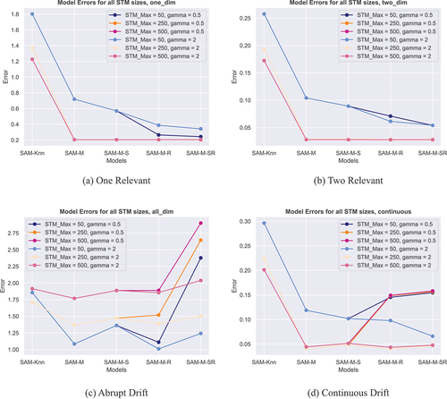
Table 3. RMSE rates on toy data sets with feature drift for all versions of SAM. Errors are given for maximum STM sizes of 50, 250 and 500 data points.

Data set	SAM	SAM-M	SAM-M-S	SAM-M-R	SAM-M-SR
STM size 50
One Relevant	$1.802$	$0.719$	$0.570$	$0.265$	$\mathbf{0}\mathbf{.243}$
Two Relevant	$0.257$	$0.104$	$0.089$	$0.071$	$\mathbf{0}\mathbf{.054}$
Abrupt Drift	$1.856$	$1.084$	$1.362$	$\mathbf{1}\mathbf{.001}$	$1.249$
Continuous Drift	$0.296$	$0.118$	$0.101$	$0.098$	$\mathbf{0}\mathbf{.069}$
STM size 250
One Relevant	$1.369$	$0.206$	$0.206$	$\mathbf{0}\mathbf{.205}$	$\mathbf{0}\mathbf{.205}$
Two Relevant	$0.1938$	$0.029$	$0.029$	$\mathbf{0}\mathbf{.028}$	$\mathbf{0}\mathbf{.028}$
Abrupt Drift	$1.712$	$1.371$	$1.471$	$\mathbf{1}\mathbf{.368}$	$1.503$
Continuous Drift	$0.223$	$\mathbf{0}\mathbf{.040}$	$0.048$	$0.043$	$0.047$
STM size 500
One Relevant	$1.227$	$0.205$	$0.205$	$\mathbf{0}\mathbf{.204}$	$\mathbf{0}\mathbf{.204}$
Two Relevant	$0.172$	$0.028$	$0.028$	$\mathbf{0}\mathbf{.027}$	$\mathbf{0}\mathbf{.027}$
Abrupt Drift	$1.914$	$\mathbf{1}\mathbf{.768}$	$1.887$	$1.799$	$2.015$
Continuous Drift	$0.201$	$\mathbf{0}\mathbf{.044}$	$0.051$	$0.047$	$0.049$

Overall, one can see, that the introduction of metric learning to SAM improves the prediction quality for all data sets and all STM sizes. The exact effects of each model on the RMSE is described in the following paragraphs.

SAM: The vanilla version of SAM is the worst performer of all tested models. Naturally, larger STM sizes correspond to better overall performance.

SAM-M: When metric learning in the form of MLKR is introduced, a significant improvement of prediction quality can be observed. This improvement is largest for data sets with static and continuously changing features. For abruptly changing features this effect diminishes but can still be observed.

SAM-M-S: Metric smoothing only has a benefit for small STM sizes on data sets with static or continuously changing features. When larger STM sizes are considered, there is no improvement in prediction quality compared to metric learning without smoothing. For data sets with abruptly changing features, one has to note, that metric smoothing actually diminishes the prediction quality in comparison to standalone metric learning.

SAM-M-R: Dimensionality reduction is not supposed to lead to any improvements in the RMSE. However, a correct reduction should not diminish the prediction quality either. In the plots, we show the results for two different reduction schemes. One, where a threshold of at least $50\mathrm{\%}$ of the relevance of the most important feature is applied and another one, where we always reduce to two dimensions. For static features, the reducing of dimensions is no problem at all, regardless of which specific reduction strategy is applied. For small sizes of the STM one can even observe a small improvement of the RMSE. Larger STM sizes do not lead to such an improvement but there is no decline either. For non-static data sets on the other hand, the outcome depends on the reduction strategy. When we constantly reduce down to two dimensions, then the results are in line with those of the static data sets. However, if a threshold is used and the number of leftover features is determined from that, then a considerable increase of the RMSE can be observed.

SAM-M-SR: The final model employs dimensionality reduction as well, but this time on a smoothed metric. The outcome for static data sets is the same as without metric smoothing. However, when the data sets with non-static features are considered the results change. Interestingly, now even the reduction strategy of always reducing down to two dimensions can yield worse results than applying the same strategy without metric smoothing. For the reduction strategy that is based on a threshold, the results are even worse. Here, it is now possible, that the RMSE increases even beyond the error of SAM without any kind of metric learning.

Evaluation of Feature Relevance

In the following, we will evaluate the outcome of the feature relevance computations for both approaches, plain metric learning and metric smoothing. To do that in adequate detail, we will consider data sets with different behavior of features separately.

Static Features Figure 2 shows four relevance plots for the Two Relevant data set. In this set, the first feature contributes $40\mathrm{\%}$ to the total relevance while the second feature contributes $60\mathrm{\%}$. These two features are plotted in blue and orange, respectively. All other features are irrelevant to the regression problem.

Figure 2. Different Relevance plots for the Two Relevant data set. (a) shows the relevance over time as computed by MLKR. (b) shows the same data as (a) but all values are normalized by the maximum value of each time step. (c) shows the relevance under a smoothed metric. (d) shows the same data as (c) but again normalized.

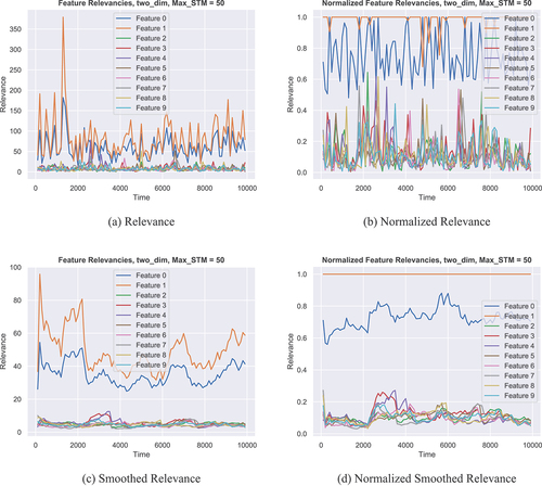
Plot (a) shows the computed relevance over time from SAM-M, a model without metric smoothing. One can see, that there is a clear difference in relevance between the first two features and the others. Also, the orange feature seems to be more relevant than the blue one for most of the time, although it sometimes can be hard to tell.

Plot (b) shows the same data as (a) but this time the relevance values are normalized by the value of the most important feature at each time step. This means that the most relevant feature at any given point in time will have the value $1$ while the others will have values below that. In this fashion, it is possible to see, that overall, the computation of the relevance is adequate, but for some points in time, the blue feature is judged as more important than the orange one, which is not in agreement with ground truth.

The other two plots, (c) and (d), show the same information as (a) and (b), but for the model SAM-M-S, meaning a model with metric smoothing. In those plots, the computed relevances are a lot smoother and also clear differences between the two relevant features can be observed now, a behavior that is in exact agreement with ground truth.

Continuous Drift: The relevance plots for the Continuous Drift data set are shown in Figure 3, where all subplots are arranged in the same way as described for Figure 2. In this set, the first feature (plotted in blue) continuously increases its relevance from $0\mathrm{\%}$ to $100\mathrm{\%}$ over the course of the data stream. At the same time, the second feature (plotted in orange) decreases its relevance from $100\mathrm{\%}$ to $0\mathrm{\%}$. All other features are irrelevant to the regression problem.

Figure 3. Different Relevance plots for the Continuous Drift data set. (a) shows the relevance over time as computed by MLKR. (b) shows the same data as (a) but all values are normalized by the maximum value of each time step. (c) shows the relevance under a smoothed metric. (d) shows the same data as (c) but again normalized.

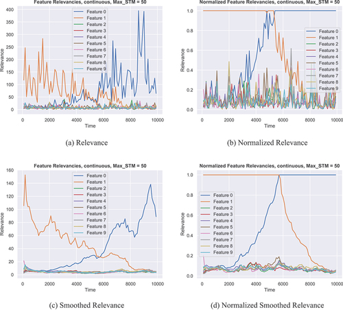
Plots (a) and (b) show the expected behavior of the relevance values over time, with a region between time points 4500 and 5500 where the two features have roughly the same relevance, cumulating in a definitive switch of both features for the rest of the data stream.

Plots (c) and (d) now show a slightly different picture. The time point at which both curves meet, is now significantly offset to the right. In other words, the time point on which both features appear to have the same relevance is much closer to the 6000 mark instead of the 5000 mark, where it should be according to ground truth. The reason for this is metric smoothing. Since, in the smoothing process, the relevance values of many past computations are taken into account, and the change of the features is continuous, the curves computed from a smoothed metric learner will display the correct behavior overall, but with a delay in time of significant events like the switching of highest relevance between the two features.

Abrupt Drift: Figure 4 shows relevance plots for the Abrupt Drift data set. In this set, only one feature is relevant at any given time, but every feature is relevant for 1000 consecutive points in time.

Figure 4. Different Relevance plots for the Abrupt Drift data set. (a) shows the relevance over time as computed by MLKR for a maximum STM size of 50. (b) shows the same as (a) but for a maximum STM size of 500. (c) shows the relevance under a smoothed metric, for a maximum STM size of 50. (d) shows the same data as (c) but again for a maximum STM size of 500.

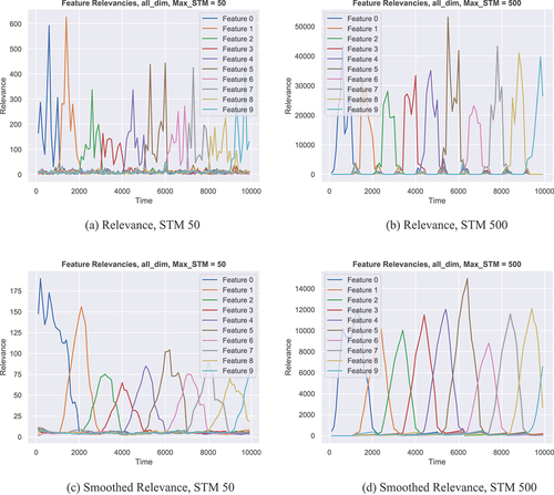
Plot (a) shows the relevance over time for a SAM-M model with a maximum STM size of 50. In comparison to that, plot (b) shows the relevance for the same model but with a maximum STM size of 500. One can observe two things from that. First, the larger the STM can potentially be, the more often it can happen that a significant number of instances in the STM has another relevant feature than the rest of the STM. This confuses the metric learner and leads to significantly higher relevance values overall, as can be seen from the little hills at the transition points of relevant features. Furthermore, larger STMs cause a similar delayed distortion of the relevance picture as the smoothed metric in the continuous example.

Plots (c) and (d) show the same as (a) and (b) but now for a model with metric smoothing. As can be seen from the plots, the smoothing process leads to the relevance picture being perceived as continuously changing instead of the abrupt changes that are given by ground truth. In addition to that, one can see that larger STM sizes exacerbate the problem of delayed relevance distortion that was already observed for the Continuous Drift data set.

Evaluation of Dimensionality Reduction

As described above, there are two different ways of adjusting to how many leftover dimensions the algorithm reduces. Using a threshold value, has the theoretical benefit of the algorithm being able to using different numbers of leftover dimensions during deployment, just in the way as they are needed. However, this strategy can also lead to problems, as visualized in Figure 5.

Figure 5. Different Dimensionality Reduction plots for the Abrupt Drift data set. All plots show a point in the grid for each feature that was left over after dimensionality reduction at any given point in time. (a) and (c) show a reduction strategy where the number of leftover features is determined by a threshold. (b) and (d) show a strategy where we always reduce down to two leftover features. Again, the top row shows the situation without metric smoothing, while the bottom row shows the other side.

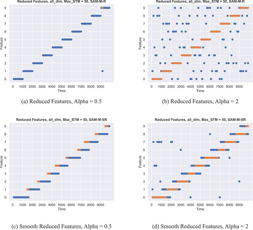
Plot (a) shows the threshold strategy under a model without metric smoothing. Here, everything is fine. The model always reduces down to only one leftover dimension and correctly weighs the right features for each point in time.

However, if the same is done for a model with metric smoothing as shown in plot (c), then the already familiar delayed relevance distortion prompts the model to reduce to incorrect features around the points of relevance transition in the stream. This in turn has an adverse effect on the prediction quality because the only feature that is important to the output gets canceled out for a significant number of points in time.

This can of course be mediated, by using a different strategy, that sets a specific number of leftover dimensions for the whole operation as shown in plot (d). Here, one can observe that while the delay effects are unchanged, through the higher number of chosen features, the correct ones are still almost always preserved.

On the other hand, the second strategy can also have negative effects if combined with a non-smoothed model as shown in plot (b). Here, no gain in prediction quality is made with respect to (a), but the number of leftover features has doubled which has a negative effect on computational cost.

Overall Evaluation of the Versions of SAM-MLKR

In the last sections, we described the behavior of the different versions of SAM with regard to multiple objectives. In summary, we come to the following conclusions.

Metric Learning: The introduction of MLKR into the SAM framework is a clear and definite improvement that in its simplest form can lead to substantial gains in prediction quality, but also enables interpretability as well as dimensionality reduction.

Metric Smoothing: The process of smoothing the metric is especially beneficial for small STM sizes but with regard to relevance interpretability it can also deliver much better insights for large STM sizes. However, this is only true for situations in which the relevance of features is stationary. As soon as non stationary features are expected to be present in a data set, one should abstain from metric smoothing because of the adverse effects of delayed relevance distortions.

Dimensionality Reduction: Metric learning can safely be used to reduce the number of dimensions whenever the data sets are stationary. In none stationary sets, it can also be used, but here, it should never be combined with metric smoothing because the delayed distortions will lead to imperfect reductions.

All in all, we will use the SAM-M-R model for the remainder of the paper, as it is best suited for the real-world task described in the next section.

Real-World Application

We created our model for an application in the Water Distribution Network (WDN) domain. In the following sections, we will describe the data, explain the objectives and present the results.

Data Set

We work on data that was generated from the L-Town Network (Vrachimis et al. 2020). This network is a benchmark WDN with three distinct areas: A, B and C, that is depicted in Figure 6(a). The largest of these areas is ’Area A,’ which forms the basis for our simulation. In this area, there are 661 consumer nodes, which are connected by a grid of 766 water pipes. In addition to that, there are 29 pressure sensors as depicted in Figure 6(b). The data are created by the simulation tool WNTR (Klise, Murray, and Haxton 2018), utilizing realistic demand patterns. We simulate different scenarios for a 3-month period, where the pressure sensors are sampled every 5 minutes. This creates data streams with 29 features and about 26,000 samples. Each scenario is unique and contains a water leak in the WDN, whose location and size differs across the different scenarios. These leaks introduce concept drift into the data which create the necessity for algorithms with corresponding capabilities. Furthermore, the scenarios contain simulated sensor faults, which break the pressure dynamics for specific input features. Sensor faults are usually simulated in one of five different ways in the literature (Vaquet et al. 2022). Sensors can put out random noise, shift to a constant output, drift to infinity, slowly converge to an arbitrary number or include an offset into their readouts. According to that, we evaluate our approach on five different scenarios that are described in Table 4.

Figure 6. L-Town Water Distribution Network as given by Vrachimis et al. (2020). (a) shows the different areas of the network. (b) shows the placement of pressure sensors inside the network.

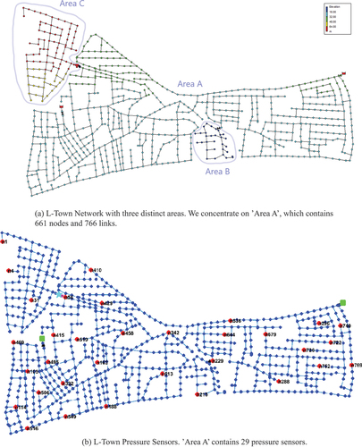
Table 4. Description of the WDN scenarios used in the real-world experiment. The last column describes how a sensor fault is simulated in the data.

Name	Dim	Size	Sensor fault
Scenario 1	28	26000	Random noise
Scenario 2	28	26000	Constant output
Scenario 3	28	26000	Drifts to infinity
Scenario 4	28	26000	Slowly converges
Scenario 5	28	26000	Offset

General Challenges

In general, real-life WDNs need to be monitored constantly, in order to ensure, that they are capable of delivering water to every consumer at all times. When leaks occur in the network, valuable drinking water is lost in potentially large quantities and the possibility of drinking water contamination becomes an issue. Therefore, leaks have to be detected and localized by the monitoring system in order to find and repair them. Since a leak in a pipe causes pressure to fall off, it changes the pressure dynamics around the leak. This fact is used to detect leaks by training virtual sensors and comparing their predictions with real-world measurements. When predictions and measurements start to deviate significantly, one can take this as an indication for a nearby leak (Eliades and Polycarpou 2012; Santos-Ruiz et al. 2019). However, since pipes are buried underground, and therefore, are not easily accessible, in practice it can take a long time until detected leaks are actually fixed. In that time, the models of the virtual sensors have to adapt themselves to the new pressure dynamics, in order to be able to detect additional leaks and to prevent reporting on the same leak over and over again. This means that some forms of incremental models have to be applied. In our last paper (Jakob et al. 2022), we showed that SAM-kNN Regression is up to that task. Since, the whole of WDN monitoring is hinged on physical sensors and their readouts, the question arises what happens if those sensors fail. Dealing with these kinds of scenarios is also an area of ongoing research (Vaquet et al. 2022).

Now, with the work in this paper, we want to combine the handling of those problems by leveraging the interpretability of SAM-MLKR.

Problem Setting

For a given scenario with 29 pressure features, we train virtual sensors for each feature by learning the pressure dynamics of a sensor from all other sensors in the network. This amounts to building a function $f_i:{\mathbb{R}}^{28}\to \mathbb{R}$ that tries to predict the pressure at the $i$th sensor based on the last pressures of all other 28 pressure sensors. We use SAM-M-R as a model for $f_i$ and utilize the feature relevance computations to detect sensor faults.

Results

The results in terms of RMSE are reported in Table 5. For any given scenario, we average the RMSE of all 29 virtual sensors as the prediction quality of a model for that scenario. We compare our old version of SAM with the new SAM-MLKR and also a version that reduces the dimensionality of the data from 28 down to 10. The results show, that SAM-MLRK outperforms the older version on all scenarios. Furthermore, we can show that it is possible to maintain the approximate level of prediction quality when we reduce the dimensionality by $65\mathrm{\%}$ which enables considerable savings in terms of computational cost.

Table 5. Average RMSE rates for different versions of SAM. SAM-M-R reduces the dimension down to 10. The RMSE values are averaged over all virtual sensors in each scenario.

Data set	SAM	SAM-M	SAM-M-R(10)
Scenario 1	$1.843$	$\mathbf{1}\mathbf{.669}$	$1.675$
Scenario 2	$1.903$	$\mathbf{1}\mathbf{.680}$	$1.688$
Scenario 3	$1.715$	$\mathbf{1}\mathbf{.493}$	$1.501$
Scenario 4	$1.822$	$\mathbf{1}\mathbf{.656}$	$1.693$
Scenario 5	$1.778$	$\mathbf{1}\mathbf{.624}$	$1.638$

Figure 7 shows the relevance computations for one virtual sensor in scenario 1. In this scenario, sensor 16 experiences a sensor fault, simulated through the output of random noise, after about half of the data stream.

Figure 7. Relevance of pressure sensors in scenario 1. (a) Relevance over time of the sensor experiencing the fault. (b) Relevance picture before the sensor fault (note, that sensor 16 is the most important). (c) Relevance picture after the sensor fault (note, that sensor 16 is the least important).

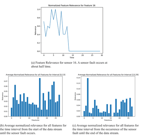
Plot (a) shows the relevance for the affected sensor over time. One can observe, that the sensor becomes irrelevant to the prediction model after the occurrence of the sensor fault.

Plot (b) shows the average normalized relevance for all features (or sensors) for the time interval from the start of the data stream until the sensor fault occurs. From that, it now becomes clear, that for the model of the virtual sensor in question, sensor $16$ was the most important input overall.

However, when compared with plot (c), which shows the same averages for the time interval from the sensor fault until the end of the stream, one can see, that from the time the sensor fault occurs, the model completely ignores sensor $16$ and instead assigns more relevance to other sensors, like sensor $2$ for example.

All in all, this shows, that sensor fault detection is possible by monitoring the feature relevances of virtual sensors in a WDN monitoring system. This kind of detection is possible for all sensor faults that completely break the pressure dynamics, like in scenarios 1–4. In scenario 5, it depends on how large the offset is. For small offsets within the same magnitude of normal values it is not possible to detect the sensor fault with feature relevance monitoring. However, when higher magnitudes are considered it becomes possible again.

Discussion and Implications

Within the SAM family of algorithms, SAM-LMNN (Kummert, Schulz, and Hammer 2023) introduced metric learning to the framework, albeit only in the context of classification problems. In our toy data experiments we showed, that the same benefits that were observed by the authors of SAM-LMNN, namely a potential improvement in prediction quality as well as the possibility to gain insights into feature relevances, can be obtained in a regression setting as well. In the same vein, we were able to show, that the metric smoothing approach from SAM-LMNN can have the same benefits on prediction quality and relevance visualization for our approach. However, in contrast to the SAM-LMNN publication, we also showed that there is a limit to the usefulness of metric smoothing, especially in the presence of feature drift and when the objective is related to localizing sudden feature drift in time. Furthermore, all SAM algorithms are usually build on distance-based methods like the kNN, which suffer from computational issues when the memories become large and the data dimension is high. The approach presented in this paper, is the first to address this issue by enabling dimensionality reduction in a cost-effective way.

With regard to the real-world application, we used our algorithm to model the pressure dynamics of a water distribution network (WDN). Usually, this kind of modeling is used to facilitate residual-based leakage detection by comparing the predictions of the model to the readouts of the sensors and raising alarms when those values deviate significantly (Eliades and Polycarpou 2012; Santos-Ruiz et al. 2019). Since, the common approaches from the literature use offline models that cannot adapt to different pressure dynamics over time, we showed in our previous publication (Jakob et al. 2022) that the vanilla version of SAM-kNN for regression works better for the problem of leakage detection than common static approaches.

In this publication, we enhanced the vanilla version through metric learning, and showed that the modeling quality of the new algorithm is higher, while the computational effort can be reduced through dimensionality reduction. Most prominently, we showed that the new approach enables gaining insights into the relevances of individual sensors in the WDN. This is important, because water network modeling completely relies on sensor measurements to obtain correct information about the network. Therefore, sensor faults that randomly occur over time, pose a big challenge for any monitoring system. Models for sensor fault detection in WDNs mostly come from control theory but not from the machine learning realm (Reppa, Polycarpou, and Panayiotou 2016, 2013). The approach in (Bouzid and Ramdani 2013) utilizes local PCAs to facilitate the task, but analogous to the state of the art in leakage detection, this method is not incremental. The most recent method for handling sensor faults is Vaquet et al. (2022). Similar to common leakage detection approaches, this algorithm is residual based. In contrast to that, we showed that sensor fault detection is also possible by monitoring the feature relevance information given by a metric learning approach over time. Since, water distribution pipes are underground and not easily accessible, replacing a broken sensor is often associated with high costs. Therefore, users want to be very sure, that a sensor in question is indeed broken and not just a false alarm. Having multiple approaches, that detect sensor faults based on entirely different information, can therefore lead to more stable predictions in practice.

Limitations and Future Work

As mentioned earlier, there is a limitation of our method for the specific case represented by scenario 5. In this scenario, a sensor fault is simulated as a numerical offset of the readouts. This simulation does not break the pressure dynamics of the sensor which makes it hard to detect for our method. In fact, when the offset is very low (e.g. in the range of only a few percent of the magnitude of the signal) then it is impossible to detect it. However, sensor faults on this scale do not pose a problem for the overall monitoring task and can therefore be neglected. On the other hand, when the offset is very large (e.g. several magnitudes greater than the signal), detection is not a problem anymore. So far we have not tested in which threshold range the switch between both possibilities occurs. Therefore, based on such an evaluation, future work could determine whether this limitation can be ignored for a live system or if the specific scenario has to be solved with a different approach.

On a more general level, we like to point out, that the original SAM framework is a strict online learner, which means that internal updates are made with every new sample that arrives from the data stream. In contrast to that, we included our extension for metric learning in batch fashion into the algorithm. This means, that the internal metric is not updated incrementally, but constantly recomputed in a predefined time interval. Therefore, the resolution in which feature drift can be observed is dependent on the size of that interval. This can be seen as a limitation of the general approach, but as of yet, it is unclear, whether incremental updates of the metric really lead to better results and whether a potential increase in performance would manifest itself for all types of feature drift. We assume that a metric computation in batch fashion yields better results for problems involving sudden feature drift, while for continuous feature drift, an incremental approach might be more suitable. However, testing this hypothesis remains the subject of future work.

Conclusion

In this paper, we presented SAM-MLKR, an extension to the popular incremental framework SAM, that utilizes metric learning. We were able to show that metric learning has a positive effect on prediction quality, provides interpretability through feature relevances and enables dimensionality reduction, which enables the dealing with high-dimensional data through savings on computational cost.

We applied SAM-MLKR to the monitoring task of WDNs, where we beat our previous approach on all fronts. In addition to that, we were able to show, that sensor faults can be detected through leveraging the interpretablility component of SAM-MLKR. Lastly, we pointed out, that SAM-MLKR on the L-Town network can retain its approximate prediction quality even after reducing the input dimensions by $65\mathrm{\%}$. For small benchmark WDNs like L-Town, this is not necessary, but in the real world, where average cities have much larger networks, the possibility of automatic dimensionality reduction can save a lot in terms of computational effort.

Disclosure statement

No potential conflict of interest was reported by the authors.

Additional information

Funding

We gratefully acknowledge funding from the VW-Foundation for the project IMPACT funded in the frame of the funding line AI and its Implications for Future Society, and funding from the European Research Council (ERC) under the ERC Synergy Grant Water-Futures (Grant agreement No. 951424).

References

- Andrade, T., B. Cancela, and J. Gama. 2020. Discovering locations and habits from human mobility data. Annals of Telecommunications 75 (9):505–1105. doi:10.1007/s12243-020-00807-x.
- Barddal, J. P., H. Murilo Gomes, F. Enembreck, and B. Pfahringer. 2017. A survey on feature drift adaptation: Definition, benchmark, challenges and future directions. The Journal of Systems and Software 127:278–94. doi:10.1016/j.jss.2016.07.005.
- Bellet, A., A. Habrard, and M. Sebban. 2013. “A survey on metric learning for feature vectors and structured data.” https://arxiv.org/abs/1306.6709.
- Bouzid, S., and M. Ramdani. 2013. “Sensor fault detection and diagnosis in drinking water distribution networks.” In 2013 8th International Workshop on Systems, Signal Processing and their Applications (WoSSPA), 378–83. Algiers, Algeria.
- Castellani, A., S. Schmitt, and B. Hammer. 2021. Estimating the electrical power output of industrial devices with end-to-end time-series classification in the presence of label noise. In Machine learning and knowledge discovery in databases. research track, ed. N. Oliver, F. Pérez-Cruz, S. Kramer, J. Read, and J. A. Lozano, 469–84. Basel, Switzerland: Springer International Publishing.
- Domingos, P., and G. Hulten. 2000. “Mining high-speed data streams.” In Proceedings of the sixth ACM SIGKDD international conference on Knowledge discovery and data mining, 71–80. Boston, Massachusetts, United States.
- Eliades, D. G., and M. M. Polycarpou. 2012. Leakage fault detection in district metered areas of water distribution systems. Journal of Hydroinformatics 14 (4):992–1005. doi:10.2166/hydro.2012.109.
- El-Zahab, S., and T. Zayed. 2019. Leak detection in water distribution networks: An introductory overview. Smart Water 4. doi:10.1186/s40713-019-0017-x.
- Göpfert, J. P., B. Hammer, and H. Wersing. 2018. “Mitigating concept drift via rejection.” In International Conference on Artificial Neural Networks, 456–67. Rhodes, Greece: Springer.
- Grbovic, M., and S. Vucetic. 2009. “Learning vector quantization with adaptive prototype addition and removal.” In 2009 international joint conference on neural networks, 994–1001. Atlanta, Georgia, United States: IEEE.
- Hammer, B., and T. Villmann. 2002. Generalized relevance learning vector quantization. Neural Networks: The Official Journal of the International Neural Network Society 15:1059–68. doi:10.1016/S0893-6080(02)00079-5.
- Hoi, S. C., D. Sahoo, L. Jing, and P. Zhao. 2021. Online learning: A comprehensive survey. Neurocomputing 459:249–89. doi:10.1016/j.neucom.2021.04.112.
- Jakob, J., A. Artelt, M. Hasenjäger, and B. Hammer. 2022. “SAM-kNN regressor for online learning in water distribution networks.” In International Conference on Artificial Neural Networks, 752–62. Bristol, United Kingdom. 10.1007/978-3-031-15934-3_62.
- Jakob, J., M. Hasenjäger, and B. Hammer. 2021. “On the suitability of incremental learning for regression tasks in exoskeleton control.” In IEEE Symposium Series on Computational Intelligence, SSCI 2021, Orlando, FL, USA, December 5-7, 2021, 1–8. IEEE. 10.1109/SSCI50451.2021.9660138.
- Klise, K. A., R. Murray, and T. Haxton. 2018. An Overview of the Water Network Tool for Resilience (WNTR). Computing and Control in the Water Industry, Ontario, Kingston, Canada.
- Kulis, B. 2012. Metric Learning: A Survey. Foundations and Trends in Machine Learning 5:287–364. doi:10.1561/2200000019.
- Kummert, J., A. Schulz, and B. Hammer. 2023. Metric learning with self adjusting memory for explaining feature drift. Submitted to SN Computer Science.
- Losing, V., B. Hammer, and H. Wersing. 2015. “Interactive online learning for obstacle classification on a mobile robot.” In 2015 international joint conference on neural networks (ijcnn), 1–8. Killarney, Ireland: IEEE.
- Losing, V., B. Hammer, and H. Wersing. 2016. “KNN classifier with self adjusting memory for heterogeneous concept drift.” In 2016 IEEE 16th international conference on data mining (ICDM). 291–300. Barcelona, Spain: IEEE.
- Losing, V., B. Hammer, and H. Wersing. 2018a. Incremental on-line learning: A review and comparison of state of the art algorithms. Neurocomputing 275:1261–74. doi:10.1016/j.neucom.2017.06.084.
- Losing, V., B. Hammer, and H. Wersing. 2018b. Tackling heterogeneous concept drift with the self-adjusting memory (SAM). Knowledge and Information Systems 54 (1):171–201. doi:10.1007/s10115-017-1137-y.
- Losing, V., B. Hammer, H. Wersing, and A. Bifet. 2020. “Randomizing the self-adjusting memory for enhanced handling of concept drift.” In 2020 International Joint Conference on Neural Networks (IJCNN), 1–8. Glasgow, United Kingdom: IEEE.
- Martinetz, T., K. Schulten, et al. 1991. A” neural-gas“network learns topologies Artificial Neural Networks. 1, 397–402 .
- Oladeji, I., R. Zamora, and T. Tjing Lie. 2021. An online security prediction and control framework for modern power grids. Energies 14 (20):6639. doi:10.3390/en14206639.
- Pau, D., A. Khiari, and D. Denaro. 2021. “Online learning on tiny micro-controllers for anomaly detection in water distribution systems.” In 2021 IEEE 11th International Conference on Consumer Electronics (ICCE-Berlin), 1–6. Berlin, Germany: IEEE.
- Reppa, V., M. M. Polycarpou, and C. G. Panayiotou. 2013. “Multiple sensor fault detection and isolation for large-scale interconnected nonlinear systems.” In 2013 European Control Conference (ECC). 1952–57. Zurich, Switzerland.
- Reppa, V., M. M. Polycarpou, and C. G. Panayiotou. 2016. Sensor Fault Diagnosis. Foundations and Trends® in Systems and Control 3 (1–2):1–248. doi:10.1561/2600000007.
- Roseberry, M., B. Krawczyk, and A. Cano. 2019. Multi-label punitive kNN with self-adjusting memory for drifting data streams. ACM Transactions on Knowledge Discovery from Data (TKDD) 13 (6):1–31. doi:10.1145/3363573.
- Rosenblatt, F. 1958. The perceptron: A probabilistic model for information storage and organization in the brain. Psychological Review 65 (6):386. doi:10.1037/h0042519.
- Santos-Ruiz, I., F.R. López-Estrada, V. Puig, and J. Blesa. 2019. “Estimation of node pressures in water distribution networks by Gaussian process regression.” In 2019 4th Conference on Control and Fault Tolerant Systems (SysTol) Casablanca, Morocco, 50–55. IEEE.
- Schneider, P., M. Biehl, and B. Hammer. 2009. Adaptive relevance matrices in learning vector quantization. Neural Computation 21 (12). doi:10.1162/neco.2009.11-08-908.
- Song, L., C. Tekin, and M. Van Der Schaar. 2014. Online learning in large-scale contextual recommender systems. IEEE Transactions on Services Computing 9 (3):433–45. doi:10.1109/TSC.2014.2365795.
- Vaquet, V., A. Artelt, J. Brinkrolf, and B. Hammer. 2022. “Taking care of our drinking water: dealing with sensor faults in water distribution networks.” In International Conference on Artificial Neural Networks, 682–93. Bristol, United Kingdom: Springer.
- Vaquet, V., and B. Hammer. 2020. “Balanced sam-knn: Online learning with heterogeneous drift and imbalanced data.” In International Conference on Artificial Neural Networks, 850–62. Bratislava, Slovakia: Springer.
- Vijayakumar, S., A. D’souza, and S. Schaal. 2005. Incremental online learning in high dimensions. Neural Computation 17 (12):2602–34. doi:10.1162/089976605774320557.
- Vrachimis, S. G., D. G. Eliades, R. Taormina, A. Ostfeld, Z. Kapelan, S. Liu, M. Kyriakou, P. Pavlou, M. Qiu, and M. M. Polycarpou. 2020. BattLeDIM: Battle of the leakage detection and isolation methods Journal of Water Resources Planning and Managment. 148: 421–438 .
- Weinberger, K., and L. Saul. 2009. Distance metric learning for large margin nearest neighbor classification. Journal of Machine Learning Research 10:207–44.
- Weinberger, K., and G. Tesauro. 2007. “Metric learning for kernel regression Journal of Machine Learning Research. 2: 612–19.
- Yamaguchi, A., S. Maya, T. Inagi, and K. Ueno. 2018. “OPOSSAM: Online prediction of stream data using self-adaptive memory.” In 2018 IEEE International Conference on Big Data (Big Data), 2355–64. Seattle, Washington, United States.
- Yang, Y., J. Che, L. YanYing, Y. Zhao, and S. Zhu. 2016. An incremental electric load forecasting model based on support vector regression. Energy 113:796–808. https://www.sciencedirect.com/science/article/pii/S0360544216310167.
- Yan, J., C. Tian, Y. Wang, and J. Huang. 2012. “Online incremental regression for electricity price prediction.” In Proceedings of 2012 IEEE International Conference on Service Operations and Logistics, and Informatics, SOLI 2012, Suzhou, China, July 8-10, 2012, 31–35. IEEE. 10.1109/SOLI.2012.6273500.
- Yipeng, W., and S. Liu. 2017. A review of data-driven approaches for burst detection in water distribution systems. Urban Water Journal 14 (9):972–83. doi:10.1080/1573062X.2017.1279191.
- Zhao, D., and Y. Sing Koh. 2020. Feature drift detection in evolving data streams. In Database and expert systems applications, ed. S. Hartmann, J. Küng, G. Kotsis, A. M. Tjoa, and C. Ismail Khalil, 335–49. Basel, Switzerland: Springer International Publishing.
- Zliobaite, I., M. Pechenizkiy, and J. Gama. 2016 An Overview of Concept Drift Applications Kacprzyk, Janusz. Studies in Big Data, 16, 91–114. Basel, Switzerland: Springer International Publishing.