A Novel Method for Reducing Vehicle Emissions Utilizing IoT-Based IS-APCPSO Algorithm

ABSTRACT

Urban road traffic network optimization based on the Internet of Things (IoT) is one of the important methods to reduce vehicle exhaust and ease traffic congestion. A two-level planning model on road traffic network optimization in IoT and the IS-APCPSO algorithm is deployed, which can effectively solve the above problems. The experimental results show that the total vehicle emissions of the proposed scheme are lower than those of traditional schemes. Moreover, the real-time perception, interactive coupling, and coordinated control of “people-vehicle-road-environment” can be achieved through the use of the IoT. We discuss the sensitivity of the model to establish a scene selection that takes into account different regional and road traffic conditions, avoiding the subjective randomness in model parameter selection. A novel multi-objective method based on IoT proposed in this paper helps to alleviate “urban diseases,” such as traffic congestion, vehicle emissions, and energy waste, and to emphasize the overall benefits of energy-saving and emission reduction in urban road networks. By setting up traffic lights reasonably and guiding the driver behavior, the integrated control and management of traffic flow and exhaust emission under multiple driving cycles are realized.

Introduction

In recent decades, the number of vehicles on the urban roads has continued to increase. However, the improvement of road capacity and the reduction of vehicle emissions have not developed at the same rate. In many cases, the improvement of road capacity does not lead to a reduction in vehicle emissions. Urban transportation still faces three major problems: traffic congestion (efficiency issues), vehicle emissions (health issues), and traffic accidents (safety issues). Motor vehicle emissions have become one of the main sources of air pollution in many cities. For example, motor vehicle emissions contribute about 40% of PM_2.5 sources in Beijing, and the total discharge of CO, HC, and NO pertaining to motor vehicle emissions is over 75%, 30%, and 50% (Shen et al. 2021). Especially when the motor vehicle is in idle state, the exhaust emission problem is more serious. Therefore, solving the problem of motor vehicle pollution in urban road networks is a complicated engineering system. This engineering challenge must be simultaneously guided from both urban road traffic supply and demand. To achieve a balance between urban road traffic supply and demand, we can use a variety of combined methods such as the information technologies, the traffic guidance system, and the Internet of Things (IoT).

Serious motor vehicle emissions pollution has led to many experts to commit to research on the subjects of urban road network traffic flow and motor vehicle emissions. Huang (2011), Huang et al. (2017), Huang et al. (2019), and Nagurney et al. (2002) have made a series of achievements in areas such as emissions modeling. The exhaust emission factor is not constant. Instead, this factor is related to vehicle type, fuel consumption, driving conditions (such as acceleration, deceleration, idling, uniform), road quality, and other factors. Additionally, some measurements on traffic management and control can also directly affect the exhaust emission factor changes, such as road widening, IoT, and signal timing optimization. Applications of IoT technologies in urban traffic network includes RFID, vehicle sensor, long-term parking calculation, weather monitoring, scheduling, and simulation. In the process of traffic management, if a sudden situation occurs on the road, the vehicle network will be prompted by the automatic detection system to select the optimal road for the driver. In the public transportation system, the IoT intelligent transportation system can be used to manage and control public transportation operations, such as electronic station signs, vehicle scheduling, and intelligent toll cards. The IoT intelligent transportation system can provide detailed and real-time information on the current status and specific performance of each vehicle (Su 2015). There have been some cases to prove that the parking difficulties can be alleviated in today’s big cities, by utilizing ultrasonic sensors, camera sensing, solar power supply, and big data in IoT (Dipti and Abhijit 2022).

The rise of IoT technology has played a crucial role in urban management in today’s information age. Some researchers opted for intelligent and efficient use of existing infrastructure through adaptive traffic management and proposed improvement measures based on Artificial Intelligence (AI), IoT, and Big Data (Asma et al. 2022). Combination of wireless sensor network and electrochemical toxic gas sensors and the use of a Radio Frequency Identification (RFID) tagging system to monitor car pollution records anytime and anywhere (Vimal et al. 2022). Antonio et al. (2023) proposed a novel Road Traffic Noise Model (RTNM), capable of dynamically assessing road traffic noise levels from reliable data (hourly traffic volumes and speed), supporting or replacing noise sensor networks.

However, the most exhaust emissions utilize fixed value models in preceding network designs (Zhang et al. 2006; Zhou 2009). The total amount of road network emissions is not only related to traffic flow but also to idle time at intersection and other factors. There is relatively little existing literature that combines traditional urban traffic optimization measures with IoT technology to study exhaust emissions reduction. In this paper, a variety of methodology combinations and strategies are discussed, and the exhaust emission rate should be considered in conjunction with the idle time. This approach can more accurately reflect real-world road network driving conditions and help to improve the accuracy of policy formulation.

Through the application of a series of traffic rules and traffic facilities that control traffic, the traffic flow in time and space is evenly distributed. This technique can effectively avoid traffic congestion and improve the traffic network efficiency. These applications, such as the IoT, can encourage traffic flow and reduce its traffic impedance, so as to achieve the purpose of adjusting the network traffic flow and uniform traffic load. The various objects can be connected and arranged by using the I0T technology and achieve intelligent and automated management. One of the main applications of current IoT is to optimize urban road traffic networks and to improve transportation management efficiency. Smart sensors of IoT have revolutionized the urban traffic with their capability of capturing physical parameters. The sensors provide vital data more precisely to the monitoring station in the applications of traffic flow control, exhaust emission, meteorological analysis, disaster management, etc. (Pankaj, Rahul, and Pradeep 2023). Several parameters, such as health loss charges, reliability, road type, and parking, can influence the road resistance function to induce change (Chen et al. 2007; Ren 2007; Wang et al. 2010; Yin 2002; Zou 2009). Based on previous research, it is necessary to discuss whether the bi-level planning model utilizing IoT is more effective for traffic flow control and exhaust emission control. In this study, the motor vehicle road resistance function is affected by road capacity increment and signal timing control parameters in IoT, which is one of the key modelling analyses.

Related Work

Traditional Models and Algorithms for Vehicle Emissions Reduction

The traditional vehicle emission models include the MOBILE and MOVES models developed by the Environmental Protection Agency, CMEM models developed by the University of Michigan and Lawrence Berkeley National Laboratory, and EMIT models developed by Cambridge Environmental Research Consultants. These models have achieved remarkable results, which are applied to many urban traffic networks. Meanwhile, many researchers proposed other models and algorithms, such as genetic algorithm (Kwak et al. 2011), discrete simultaneous perturbation stochastic approximation, artificial neural network recognition algorithm, equal saturation optimization decomposition algorithm, and hybrid algorithm perform parameter correction and optimization (Gong 2011; Park et al. 2009; Wei 2011; Xu et al. 2016; Xu et al. 2016; Yang et al. 2013; Yang 2014; Zhang et al. 2015; Zhang et al. 2016). With the expansion of the road network scale, the real-time requirements of exhaust emission monitoring, and the development of IoT, the superiority of the group intelligence algorithms, such as the particle swarm optimization (Liu et al. 2017), has gradually emerged, and is worthy of further study.

Driving behavior adjustment, signal timing optimization (Coensel et al. 2011; Noland 2001; Stevanovic et al. 2007), vehicle speed management, increasing road capacity (Rakha and Ann 2004), and setting up bus lanes (Chen et al. 2007) have an effect on reducing motor vehicle exhaust emissions. However, the Braess Paradox may occur in the design of urban road networks. In some cases, adding a new road to the urban road network may actually increase everyone’s travel time. This phenomenon is consistent with the argument mentioned in Nash equilibrium that “the aggregation of intelligent choices by individuals is not actually the optimal solution”. In particular, when there are multiple optimization goals, they often need to be consolidated to eliminate contradictions and achieve effective integration and optimization.

For the short-term treatment of motor vehicle exhaust emissions, adopting a combination of multiple methods may be more urgent and effective. The applications of IoT, cloud computing, and big data will impact energy conservation and emission reduction. With the connection and interaction of traffic monitoring equipment, intelligent traffic signal lights, and intelligent navigation systems, the real-time traffic flow and road conditions can be obtained. Thus, real-time traffic flow and road conditions can be obtained, enabling real-time adjustment of traffic signals and intelligent planning of traffic routes, improving traffic efficiency, reducing traffic congestion and vehicle emissions. With the continuous progress of new technology, the integration of big data and the IoT has become an indispensable stage in the development of smart cities. Big data refers to a vast collection of data that contains rich information and value.

The IoT is a system that connects items and devices through the internet, achieving information sharing and intelligence. The quantitative research on the emission reduction of motor vehicle emissions in the IoT environment is still relatively small and mainly concentrated in the field of microscopic monitoring (Guerrero et al. 2015; Palconit and Neuz 2017; Sarkar et al. 2018; Tu et al. 2017; Vong et al. 2014). Darwish (2022) proposed a congestion-aware decision-driven architecture for information-centric Internet-of-Things applications, which has been proven that the proposed architecture significantly surpasses state-of-the-art approaches in terms of both quality of traffic information (QoI) and quality of service (QoS) especially during congested situations. Hepsiba D. et al. (2021) presented an idea about pollution and vehicle control based on Internet of Things (IoT), and sensors, communication network, micro-controller, and server have been used for vehicle performance and their pollution control. Their experimental investigations with IoT system have been proven to be more effective compared to the absence of IoT. Therefore, the combination of methods and IoT technology to construct a multi-view exhaust emission model can meet the needs of air quality management with different scales and precisions. Additionally, this combination is envisioned to contribute to intelligent perception and fine management, which warrants further research.

Novel Framework for Vehicle Emissions Reduction in the IoT

The unbalanced supply and demand of urban transport networks is one of the cruxes and causes of various traffic problems. The traditional urban traffic network optimization problem is usually an optimal investment decision problem, which refers to expanding or renovating road sections while considering the behavior choices of traffic travelers under certain investment constraints, in order to achieve the optimal goal of urban traffic network system. Due to the mutual influence between government departments and traffic travelers involved in the decision-making process of urban traffic network, it is a typical two-level decision-making problem. With the exchange of various information, the functions of IoT such as vehicle recognition, positioning, tracking, intelligent monitoring, and management are achieved. In recent years, the IoT technology has been widely applied in the urban traffic network for achieving intelligent transportation management. At present, the two applications of IoT in urban road network optimization are intelligent control and dynamic traffic signal. The balanced model of supply and demand in the IoT is shown in Figure 1.

Figure 1. The balance model of supply and demand in the IoT.

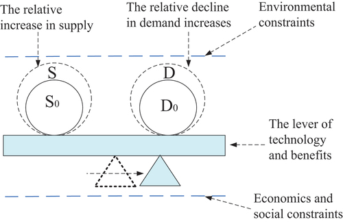
The model focuses on the needs and supply, through the simultaneous balance of traffic, social, and environmental relations, and can alleviate the contradictions between society and nature. The primary and derivative demand of traffic flow can be more effectively realized under certain constraints such as investment and exhaust emissions, by regulating the effect of the technical and beneficial lever based on IoT. The applications of IoT in urban road traffic include sensor detection (traffic flow and exhaust emissions, etc.), vehicle network, equipment maintenance, traffic accident handling, medical emergency treatment for traffic accidents, parking management, and intelligent driving scenario application support (Liu and Ke 2023). The effect of the technical and beneficial lever based on IoT mainly refers to the costs and benefits (including direct and indirect benefits) generated by investing in the IoT in urban road traffic systems (including fixed devices, mobile devices, network devices, software, etc.).

The guidance of “balance of supply and demand” is applied through the situational awareness provided by the technical and beneficial lever based on the IoT. The demand side through the signal controls and regulates travel, eases traffic congestion, reduces traffic emission, and then achieves a balanced distribution. Regarding the supply side, through the appropriate IoT technology application or broadened road, we can improve the capacity to ease traffic pollution, and then form economic and environmental benefits that constitute a win-win situation.

The policy tools for reducing vehicle emissions in urban road networks are divided into three types: supply, demand, and technology. The mechanism is shown in Figure 2. Based on IoT technology and new generation information technology rather than traditional environmental control methods, these measures make exhaust emission monitoring in urban road networks more efficient, transparent, and safer.

Figure 2. The mechanism of three policy tools.

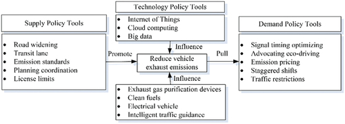
Supply policy tools include road widening, transit lane, emission standards, planning coordination, and license limits. Demand policy tools include signal timing optimization, emission pricing, staggered shifts, and traffic restrictions. Technology policy tools include IoT, cloud computing methods, big data technology, exhaust gas purification devices, and intelligent traffic guidance. The reduction system architecture of automotive emission based on the IoT is divided into three layers: intelligent perception, information integration, and application services (Figure 3).

Figure 3. The reduction system architecture of automotive emission based on the IoT.

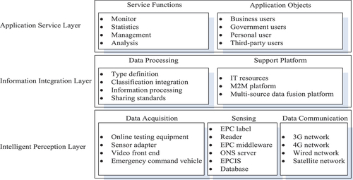
The first layer is the intelligent perception layer, which includes three sub-layers of data acquisition, sensing, and data communication. For example, in the collection and prediction of traffic flow data, a flexible framework for origin–destination matrix (ODM) inference using data from IoT and other sources has been proven to be more accurate than traditional Origin–Destination flows prediction (Sun et al. 2023). The second layer is the information integration layer, which includes two sub-layers of data processing and support platforms. By connecting object to the information network, the more reliable information exchange and sharing can be carried out anytime based on the integration of IoT and other communication networks. Utilize various intelligent computing technologies to analyze and process massive perceptual data and information, achieving intelligent decision-making and control on urban traffic network (Sun et al. 2010). The third layer is the application service layer, which contains two sub-layers of application objects and service functions. For example, a prototype is proposed for a traffic management system using IR sensors, Arduino (that is an open-source electronic prototype platform), serial to the parallel shift register, and LED displays, which is beneficial for alleviating intersection congestion and reducing vehicle emissions (Bhavana et al. 2023).

Model and Algorithms

General Definitions

The bi-level planning is generally used to describe the problem of traffic network design. In this article, we will integrate IoT technology with traditional bi-level planning methods to achieve urban road traffic optimization. The goal of upper-level planning is to minimize the total amount of motor vehicle emissions in the urban road network. Its constraints are road widening costs and IOT investment and operating costs. The goal of lower-level planning is to meet the minimum road impedance of different road users for travel needs. Its constraints are road capacity and OD traffic flow. Road widening and signal timing optimization, is a continuous variable transport network of decision variables (Gao et al. 2000). Due to the fact that the upper-level planning model should consider the road traffic volume of different vehicle types in every road section, we select a multi-vehicle user balance model for different road sections in the lower-level planning model.

In the process of optimizing urban road traffic networks, the goal of a model is to minimize all traffic emissions with the constraints of total cost and traffic impedance, but traffic management departments cannot control the travel choice behavior of travelers. In order to minimize their travel costs or to maximize their utility, travelers adjust their travel mode and route choice at any time with changes of characteristics in the urban road traffic network. The improvement of urban road traffic characteristics mentioned above can be achieved by using IoT technology. For example, we can collect and analyze various effective internet of vehicles information through GPS, RFID, QR, and sensors anytime and anywhere. In this way, it can be applied to various advanced systems such as intersection signal control systems, variable lane signal control systems, and regional traffic guidance systems. Moreover, urban road traffic optimization goals can be achieved through intersection sensing signal control, variable lane control, dynamic traffic guidance, and parking guidance in IoT environment. These are also the main differences between this paper and other existing research results.

The basic assumptions are as follows:

1. Consider the exhaust emissions of motor vehicles, regardless of the manner of mixed transport, such as motorcycle exhaust emissions.

2. From the medium perspective, only consider the motor vehicle driving conditions of uniform and idle state, regardless of the impact of acceleration and deceleration respective to exhaust emissions.

3. An assumption is that the speed of the vehicle on each section and slope are relatively fixed.

4. Non-signal control of the intersection does not take into account the motor vehicle idling time.

5. Signalized intersection control is independent, as signal timing is fixed with time.

6. Each signal cycle consists only of the green signal and the red light signal.

7. In terms of the intersection, the average communication delay time is equal to the motor vehicle parking idling time.

8. The exhaust emissions are assumed to consist only of CO, HC, and NO.

9. Ambient temperature is assumed not to impact the exhaust emissions vehicles.

The variables are defined as follows:

• A: Network section set, $\mathit{a}\in \mathit{A}$ is any section.

• J: Network intersection set, $\mathit{j}\in \mathit{J}$ is any intersection.

• $\mathit{E}{T}_{\mathit{a},\mathit{i},\mathit{j}}$: The total amount of pollutants emitted by the i kind pollutant in the urban road network at intersection j and section a. i=1 represents contaminant CO; i=2 represents contaminant HC; and i=3 represents contaminant NO.

• ${\mathit{\omega }}_i$: The proportion of the pollutant contribution of the i type of pollutant.

• $R_{\mathrm{i},\mathrm{j}}^{\mathrm{P}\mathrm{C}\mathrm{U}}\left({\mathrm{d}}_{\mathrm{a},\mathrm{j}}\right)$: The unit time idling rate of discharge at the intersection j for a standard vehicle.

• $F_{\mathrm{a},\mathrm{i}}^{\mathrm{P}\mathrm{C}\mathrm{U}}\left({\mathrm{L}}_{\mathrm{a}},{\mathrm{t}}_{\mathrm{a}}\right)$: The unit mileage of uniform emission factor on the section a for the standard vehicle.

• $d_{\mathrm{a},\mathrm{j}}\left({\mathrm{x}}_{\mathrm{a},\mathrm{j}},{\mathrm{y}}_{\mathrm{a}},{\mathrm{T}}_{\mathrm{j}},{\mathit{\lambda }}_{\mathrm{a}}\right)$: The intersection of idle time for the standard vehicle, which is the function with variables such as traffic flow, increment of road capacity, signal cycle, and green ratio.

• $t_a\left(x_a,y_a,{\lambda }_a\right)$: Link impedance function for standard vehicle, which is the function with variables such as traffic flow, increment of road capacity, and green ratio. It is also known as vehicle travel time.

• $L_a$: The length of section a.

• ${\mathrm{x}}_{\mathrm{a},\mathrm{j}}\left({\mathrm{y}}_{\mathrm{a}},{\mathrm{T}}_{\mathrm{j}},{\mathit{\lambda }}_{\mathrm{a}}\right)$: Traffic flow on section a, which is a function of the increment of road capacity, signal cycle, and green ratio.

• $y_a$: The increment of road capacity for the section a.

• $T_j$: The signal cycle length for the intersection j.

• ${\lambda }_a$: The green ratio of the entrance lane corresponding for the intersection a.

• ${\theta }_1$: The weight of pollution contribution at the intersections in the road network.

• ${\theta }_2$: The weight of pollution contribution on the section in the road network.

• $\mathit{c}{w}_1$: The conversion coefficient of vehicle emissions and the traffic system impedance with the same unit.

• $\mathit{c}{w}_2$: The conversion coefficient of the total cost and the traffic system impedance with the same unit. The total cost includes road widening cost and IoT cost.

Vehicle Emissions Model in Urban Road Network

Driving conditions of motor vehicles generally include uniform velocity, acceleration, deceleration, and idling in four states. In the process of actual urban road driving, at the intersection in idle state, the contribution rate of vehicle emissions is the highest (Sha 2007). When the intersection forms a queuing phenomenon due to signal control, the degree of motor vehicle pollution increases. Therefore, the discussion of the model of motor vehicle pollution emission in urban road networks under multiple operating conditions is highly beneficial. This relationship is composed of two factors, the idle emission at the intersection and the uniform discharge of the section, as shown in equations (1) to (3):

(1) $\mathit{E}{T}_{\mathit{a},\mathit{i},\mathit{j}}={\sum }_{\mathit{a}\in \mathit{A},\mathit{j}\in \mathit{J}}{\sum }_{i=1}^3{\omega }_i({\theta }_1\mathit{E}{I}_{\mathit{a},\mathit{i},\mathit{j}}+{\theta }_2\mathit{E}{S}_{\mathit{a},\mathit{i},\mathit{j}})$(1)

(2) $\mathit{E}{I}_{\mathit{a},\mathit{i},\mathit{j}}={\sum }_{\mathit{a}\in \mathit{A},\mathit{j}\in \mathit{J}}{x}_{\mathit{a},\mathit{j}}\left(y_a,T_j,{\lambda }_a\right)\times R_{i,j}^{PCU}\left(d_{\mathit{a},\mathit{j}}\right)\times d_{\mathit{a},\mathit{j}}\left(x_{\mathit{a},\mathit{j}},y_a,T_j,{\lambda }_a\right)$(2)

(3) $\mathit{E}{S}_{\mathit{a},\mathit{i},\mathit{j}}={\sum }_{\mathit{a}\in \mathit{A}}{x}_{\mathit{a},\mathit{j}}\left(y_a,T_j,{\lambda }_a\right)\times F_{a,i}^{PCU}\left(L_a,t_a\right)\times L_a$(3)

EI_a,i,j represents the total amount of pollution emissions when the motor vehicle is in the idle state at the intersection. ES_a,i,j represents the total amount of pollutant discharged when the motor vehicle is in a uniform state on the section. Three kinds of pollutants discharged from motor vehicle exhaust have different effects on the urban environment. Therefore, the weight can be calculated based on the expert scoring method. For example, the proportion of pollution contribution for CO is 0.7. The proportion of pollution contribution for HC is 0.15. The proportion of pollution contribution for NO is 0.15 (Yu et al.2008). $R_{\mathrm{i},\mathrm{j}}^{\mathrm{P}\mathrm{C}\mathrm{U}}\left({\mathrm{d}}_{\mathrm{a},\mathrm{j}}\right)$ denotes the idling rate of discharge, which is not a constant and is functionally influenced in terms of idle time. $F_{\mathrm{a},\mathrm{i}}^{\mathrm{P}\mathrm{C}\mathrm{U}}\left({\mathrm{L}}_{\mathrm{a}},{\mathrm{t}}_{\mathrm{a}}\right)$ denotes the uniform emission factor, which is functionally influenced by variables, such as section length and link impedance.

The idling rate of discharge is a function of the idling time, and the idle emission rate of CO, HC, and NO is the form of the piecewise function, as shown in equations (4)-(6).

(4) $R_{co,j}^{PCU}\left(d_{\mathit{a},\mathit{j}}\right)=\left\{\begin{array}{c}-5.965252+151.0967/d_{\mathit{a},\mathit{j}}\begin{array}{cc}\mathit{\hspace{0.17em}}& \left(0<d_{\mathit{a},\mathit{j}}\le 24\mathit{s}\right)\end{array}\\ 0.330443\begin{array}{cc}\mathit{\hspace{0.17em}}& \left(d_{\mathit{a},\mathit{j}}>24\mathit{s}\right)\end{array}\end{array}\right.$(4)

(5) $R_{HC,j}^{PCU}\left(d_{\mathit{a},\mathit{j}}\right)=\left\{\begin{array}{c}0.285907+3.487390/d_{\mathit{a},\mathit{j}}\begin{array}{cc}\mathit{\hspace{0.17em}}& \left(0<d_{\mathit{a},\mathit{j}}\le 24\mathit{s}\right)\end{array}\\ 0.431215\begin{array}{cc}\mathit{\hspace{0.17em}}& \left(d_{\mathit{a},\mathit{j}}>24\mathit{s}\right)\end{array}\end{array}\right.$(5)

(6) $R_{N{O}_x,\mathit{j}}^{\mathit{PCU}}\left(d_{\mathit{a},\mathit{j}}\right)=\left\{\begin{array}{c}-0.141126+2.734943/d_{\mathit{a},\mathit{j}}\begin{array}{cc}\mathit{\hspace{0.17em}}& \left(0<d_{\mathit{a},\mathit{j}}\le 18\mathit{s}\right)\end{array}\\ 0.0108\begin{array}{cc}\mathit{\hspace{0.17em}}& \left(d_{\mathit{a},\mathit{j}}>18\mathit{s}\right)\end{array}\end{array}\right.$(6)

The emission factor model uses the Traffic Network Study Tool Version 7F (TRANSYT-7F), which is a traffic signal system simulation and optimization program. The method for emission factor value in the TRANSYT-7F has been widely applied, although many scholars have made some improvements on the model for a long time. So, the emission factor model is shown in equation (7):

(7) $F_{a,i}^{PCU}=\frac{B_i{e}^{C_i{v}_a}}{D_i{v}_a}$(7)

The variable $v_a$ denotes the average velocity on the section a. $B_i$, $C_i$and $D_i$ are functionally constant for the type of pollutant i, and the values are: $B_1$=11.14272, $C_1$=0.047772, $D_1$=3280.8. An assumption is that the speed of the vehicle on each section and slope is relatively fixed. Additionally, the driving speed of the vehicle can be obtained through the length of the road divided by the vehicle travel time. Therefore, equation (7) can be rewritten as equation (8):

(8) $F_{a,co}^{PCU}\left(L_a,t_a\right)=\frac{11.14272e^{0.047772\frac{L_a}{t_a\left(x_a,y_a,{\lambda }_a\right)}}}{3280.8\frac{L_a}{t_a\left(x_a,y_a,{\lambda }_a\right)}}$(8)

Idle Time and Impedance Function

The increment of road capacity $y_a$ signal cycle $T_j$ and green ratio ${\lambda }_a$ will affect the idle time and impedance function of the vehicle. The fifth edition of the Highway Capacity Manual (HCM2010) published by the US Highway Research Board expands the evaluation methods for the capacity of various transportation facilities such as roads, interchanges, roundabouts, and road intersection channelization. HCM2010 provides an intersection signal control delay model, which is an effective delay model that has been widely applied. The model consists of three parts: uniform delay, incremental delay, and initial queuing delay, as shown in equation (9):

(9) $\mathit{d}=\frac{0.5\mathit{T}{\left(1-\mathit{\lambda }\right)}^2}{1-\left[\mathit{min}\left(1,\mathit{X}\right)\mathit{\lambda }\right]}\times \mathit{PF}+900C_L\left[\left(\mathit{X}-1\right)+\sqrt{{\left(\mathit{X}-1\right)}^2+\frac{8\mathit{KIX}}{T{C}_L}}\right]+d_3$(9)

T is the signal cycle. λ is the green ratio. X is the saturation. PF is the correction coefficient of the uniform delay, which represents the signal linkage effect, and this coefficient is recommended to a default value of 1. CL is the analysis cycle time, which is generally set to 0.25 h. K is the correction factor is dependent on the control setting, which is 0.5 for the timing signal. I is the adjustment correction factor for upstream vehicles, which is 1.0 for independent signal intersection. $d_3$ represents the impact of the initial queuing vehicle at the beginning of the analysis period based on the arrival of the vehicle, for which the recommended default value is 0:

(10) $d_{\mathit{a},\mathit{j}}=\frac{0.5T_j{\left(1-{\lambda }_a\right)}^2}{1-\left[\mathit{min}\left(1,X_a\right){\lambda }_a\right]}$(10)

$X_a$ is the saturation of section a. This relationship assumes that the vehicles arrive uniformly, regardless of the vehicle randomness of their arrivals and supersaturated queuing. Considering the influence of road capacity, saturation flow rate, and green ratio, $X_a$ can be obtained as equation (11):

(11) $X_a=\frac{q_a}{C_a}=\frac{q_a}{\left(S_a+y_a\right){\lambda }_a}$(11)

$q_a$ is traffic flow. $C_a$ is road capacity. $S_a$ is saturated flow rate as follows:

(12) $d_{\mathit{a},\mathit{j}}\left(x_{\mathit{a},\mathit{j}},y_a,T_j,{\lambda }_a\right)={\varphi }_j\times \frac{0.5T_j{\left(1-{\lambda }_a\right)}^2}{1-\left[\mathit{min}\left(1,\frac{{\mathit{x}}_{\mathit{a},\mathit{j}}\left(y_a,T_j,{\lambda }_a\right)}{\left(S_a+y_a\right){\lambda }_a}\right){\lambda }_a\right]}$(12)

Regarding equation (12), $d_{\mathit{a},\mathit{j}}\left(x_{\mathit{a},\mathit{j}},y_a,T_j,{\lambda }_a\right)$ is the model function of the idle time for the intersection. $x_{\mathit{a},\mathit{j}}\left(y_a,T_j,{\lambda }_a\right)$ is the traffic flow on section a. ${\varphi }_j$ is the 0–1 variable for describing the network intersection characteristics, ${\varphi }_j$=1 indicates the signal control intersection, and ${\varphi }_j$= 0 indicates the non-signal control intersection.

The traffic impedance function of BPR model is proposed by the Bureau of Public Roads of the United States, which has been widely used in the traffic planning, as shown in Equation (13):

(13) $\mathit{t}\left(\mathit{q}\right)=t_0\left[1+\mathit{\alpha }{\left(\mathit{q}/\mathit{c}\right)}^{\beta }\right]$(13)

Traffic impedance includes road section impedance and node impedance. This model applies $\mathit{t}\left(\mathit{q}\right)$ as the time for the traffic flows; $\mathit{q}$ for the road section; $t_0$ as the zero flow time; and c for the road capacity. Generally, α= 0.15, β= 4.0.

The impedance function is the driving time of the vehicle on the road section, which is affected by the increment of road capacity and green ratio, as follows:

(14) $t_a\left(x_a,y_a,{\lambda }_a\right)=t_a^0\left\{1.0+\mathit{\alpha }{\left[x_a/{\lambda }_a\left(S_a+y_a\right)\right]}^{\mathit{\beta }}\right\}$(14)

$t_a^0$ is the free flow time, and ${\lambda }_a=1$ indicates that the signal intersection has no entrance lane and does not consider the influence of the green ratio on the impedance function.

Bi-level Planning Model

A series of traffic management measures are designed in the IoT environment to influence the generalized impedance value of the path (e.g., delay, cost), thereby promoting the travelers in accordance with the changes in impedance to re-adjust their travel path. On the basis of the constructed intelligent monitoring system in IoT, a traffic guidance system based on intelligent transportation facilities is established in some cities, to provide more accurate and convenient traffic guidance services for travelers and alleviate traffic congestion.

For a long time, traditional vehicle-to-vehicle communication-based approaches cannot accurately estimate the vehicle emission degree and density of traffic congestion. The traffic signaling systems having a predetermined fixed operation time cannot effectively guide the traffic flow changing over time. So, long traffic queues and a large number of vehicle emissions are generated at the road crossings (Pampa and Firoj 2018). Intelligent traffic congestion control system based on the IoT has been used in many urban traffic management systems, which dynamically sets the signal operation time based on the measured values of traffic congestion density.

When traffic planners and managers realize the goal of system optimization (SO), the travelers can still travel according to the user equilibrium (UE) principle. The traffic allocation in the transportation network follows Wardrop first principle and Wardrop second principle. Wardrop first principle assumes that all travelers independently make decisions that ensure their travel time is minimized. This network traffic distribution state is called user equilibrium (UE). Wardrop second principle assumes that the travel of all travelers can ensure the minimum total time of the entire network. This network traffic distribution state is called system optimization (SO). The Wardrop first principle and the second principle (UE and SO perfect unity) form a win-win situation.

The realization principle is mainly embodied by a two-layer cycle, as shown in Figure 4. The inner loop reflects the path selection behavior of the travelers, which involves the interaction between the flow and the impedance until the user equilibrium state is reached. The outer cycle reflects a series of traffic management and control measures in the IoT environment that affect the travel behavior of the travelers to ultimately achieve the decision-making process of motor vehicle pollution control objectives.

Figure 4. The principle of emission reduction targets in the IoT.

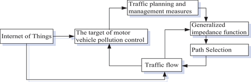
The principles of the goal can be regarded as a typical Stackelberg game, using the master-subordinate hierarchical decision-making method to solve the problem and achieve the goal by constructing the bi-level programming model. The bi-level programming model is an ideal tool to describe this kind of problem, which can meet the requirements of the overall coordination and management in the optimization of the traffic network. This model can also reconcile the contradiction between the comprehensive goal of the traffic planner, the manager, and the individual choice of the traveler. The upper model can be described as traffic planners or managers in the IoT from the system perspective to achieve the goal of reducing vehicle emissions. The lower-level planning model can be described as the behavior of choosing the travel path freely in a series of traffic management measures.

Traffic monitoring results show that automobile emission is heavy on narrow roads. The narrowing of the road is not conducive to the rapid spread of motor vehicle exhaust, this observation will cause an increase in local area pollution (Sun 2010). In order to broaden the urban road networks, we should consider the economic and environmental benefits and determine the optimal balance between them.

The parameters for incremental road capacity are adopted in the paper. The perspective of reasonable guidance of traffic demand based on signal timing optimization of traffic management measures is applied. In order to reduce the motor vehicle emissions at the intersection, we use two parameters of the signal cycle and green ratio to characterize the model. By controlling the cost of road widening and IoT to a certain extent, the whole vehicle emissions tend toward minimum. The cost of road widening includes the cost of increasing the number of lanes, upgrading the road grade, and installing road facilities. The cost of IoT mainly includes network costs, terminal costs, and maintenance costs. From the perspective of different investors, the investment cost of IoT includes the construction cost of IoT infrastructure (usually borne by government departments), the research and development cost of IoT technology (usually borne by industry associations and large institutions), and the application and daily maintenance of IoT (usually shared by government departments, industry associations, and company or individuals). In addition, the investment and income of the IoT is related to whether the network can access enough terminals. The more types and quantities of applications, the more profits are generated to the whole urban road network. The investment is usually large in the early stage of building IoT infrastructure, and the investment is relatively low in the later stage of IoT technology research, application, and maintenance. That is to say, with the widespread application of a large number of IoT technologies, their unit costs are lower. The development of IoT to a certain extent will enhance the marginal effect of its investment.

The upper-level planning model is developed with decision variables $\left({\mathrm{y}}_{\mathrm{a}},{\mathrm{T}}_{\mathrm{j}},{\mathit{\lambda }}_{\mathrm{a}}\right)$, as shown in equations (15)-(20):

$min\mathit{Z}\left(y_a,T_j,{\lambda }_a\right)=$

(15) ${\sum }_{\mathit{a\epsilon A}}{t}_a\left(x_a,y_a,{\lambda }_a\right)x_a+\mathit{c}{w}_1{\sum }_{\mathit{a\epsilon A},\mathit{j\epsilon J}}\mathit{E}{T}_{\mathit{a},\mathit{i},\mathit{j}}+\mathit{c}{w}_2{\sum }_{\mathit{a\epsilon A},\mathit{j\epsilon J}}\mathit{Cos}{t}_{\mathit{Total}}$(15)

(16) $\mathit{s}.\mathit{t}.\mathit{Cos}{t}_{\mathit{Total}}\le \mathit{Quota}$(16)

(17) $T_{\mathit{min}}\le T_j\le T_{\mathit{max}}$(17)

(18) ${\lambda }_{\mathit{min}}\le {\lambda }_a\le {\lambda }_{\mathit{max}},\mathit{a\epsilon A}$(18)

(19) ${\sum }_{a\epsilon A_j}{\lambda }_a=1,A_j\subset \mathit{A}$(19)

(20) $y_a\ge 0,\mathit{a}\in \mathit{A}$(20)

Equation (15) is a multi-objective function of the upper-level planning model, which shows that the total amount of vehicle exhaust emissions in the urban road network is the smallest with the minimum system total impedance and the total cost. The total cost includes road widening cost and IoT cost. The conversion coefficient is $\mathit{c}{w}_1$ between vehicle emissions, and the traffic system impedance is dimensionless. The conversion coefficient is $\mathit{c}{w}_2$ between the total cost and the traffic system impedance is also dimensionless. The proportion between the total amount of motor vehicle emissions control and the total cost is controlled by $\mathit{c}{w}_2$. There are two effects of $\mathit{c}{w}_2$: the weighting coefficient as the objective function and the dimension conversion factor. Equation (16) is a constraint that indicates that the total cost is limited by the investment budget. Equation (17) is a constraint that designates the signal period is constrained by the upper and lower limits. Equation (18) is a constraint indicating that the green ratio is constrained by the upper-level and lower-level limits. Equation (19) is a constraint specifying that the sum of the green ratios for all the entrances at the intersection is 1. Equation (20) is a constraint stipulating that the increment of road capacity has a non-negative constraint.

$\mathrm{Cos}{\mathrm{t}}_{\mathrm{Total}}$ is composed of road widening cost $\mathrm{Cos}{\mathrm{t}}_{\mathrm{Rw}}$ and IoT cost $\mathrm{Cos}{\mathrm{t}}_{\mathrm{IoT}}$, as shown in Equation (21). $\mathrm{Cos}{\mathrm{t}}_{\mathrm{Rw}}$ is the function of road widening cost, which has variables such as increment of road capacity ${\mathrm{y}}_a$ and the coefficient ${\mathit{\eta }}_a$ (Gao and Song 2002), as shown in equation (22). $\mathrm{Cos}{\mathrm{t}}_{\mathrm{IoT}}$ is the cost of IoT, assuming that the traffic flow is equal to the traffic volume, regardless of the type of goods and recall costs, which consist of variable costs and fixed costs (Wu et al. 2011; Wang and Du 2016), as shown in equation (23). The parameter TCF represents the technical complexity, whose value is between 0 and 1. The parameter FR indicates a fixed recovery rate. The value of 0 means that the chips can be recycled in all, on the other hand, the value of 1 means that the chips cannot be recycled. The parameter ${\mathrm{C}}_{\mathrm{Chip}}$ characterizes a single chip cost, and ${\mathrm{C}}_{\mathrm{Ma}}$ symbolizes the maintenance cost of the IoT in use. The parameter ${\mathrm{C}}_{\mathrm{Fi}}$ signifies the fixed costs of IoT implementation, such as the installation of radio frequency identification, video surveillance, and sensor technology hardware costs. ${\mathrm{F}}_{\mathrm{vol}}$ denotes the freight volume; n indicates the number of line traffic surveys; NRC represents the traffic non-repetition coefficient; $\mathrm{Rat}{\mathrm{e}}_{\mathrm{ul}}$ signifies unloaded ratio; AT shows the average tonnage of the vehicle; $\mathrm{Rat}{\mathrm{e}}_{\mathrm{ut}}$ designates the utilization ratio of heavy vehicle (Peng et al. 1997), as shown in equation (24):

(21) $\mathit{Cos}{t}_{\mathit{Total}}=\mathit{Cos}{t}_{\mathit{Rw}}+\mathit{Cos}{t}_{\mathit{IoT}}$(21)

(22) $\mathit{Cos}{t}_{\mathit{Rw}}=1.5\times {\left(y_a\right)}^2\times {\eta }_a$(22)

(23) $\mathit{Cos}{t}_{\mathit{IoT}}=\mathit{TCF}\times \left(C_{\mathit{Chip}}\times \mathit{FR}+C_{\mathit{Ma}}\right)\times F_{\mathit{vol}}+C_{\mathit{Fi}}$(23)

(24) $F_{\mathit{vol}}=\mathit{n}\times x_{\mathit{a},\mathit{j}}\left(y_a,T_j,{\lambda }_a\right)\times \mathit{NRC}\times \mathit{Rat}{e}_{\mathit{ul}}\times \mathit{AT}\times \mathit{Rat}{e}_{\mathit{ut}}$(24)

The traffic flow $x_{\mathit{a},\mathit{j}}\left(y_a,T_j,{\lambda }_a\right)$ in the motor vehicle pollution control is obtained from the lower-level planning model. We can measure the real time road traffic congestion and measure the vehicle emissions in IoT using RFID reader, sensor detector, wireless router, wireless coordinator, map software, and GSM technology. The generalized road impedance function is affected by traffic flow, road capacity, signal cycle, and green signal ratio. Therefore, the user equilibrium distribution model is modified as the following lower-level planning model:

(25) $\underset{x}{min}\sum _{\mathit{a}\in \mathit{A},\mathit{j}\in \mathit{J}}\underset{0}{\overset{x_a}{\int }}\left[t_{\mathit{a},\mathit{j}}\left(\mathit{\omega },y_a,T_j,{\lambda }_a\right)\right]\mathit{dw}$(25)

(26) $\begin{array}{cc}\mathit{s}.\mathit{t}.& \sum _k{f}_k^{rs}=q_{\mathit{rs}}\begin{array}{cc}\mathit{\hspace{0.17em}}& \mathrm{\forall r},\mathit{s}\end{array}\end{array}$(26)

(27) $x_a=\sum _r\sum _s\sum _k{f}_k^{rs}{\delta }_{ak}^{rs}\begin{array}{cc}\mathit{\hspace{0.17em}}& \mathrm{\forall a}\in \mathit{A}\end{array}$(27)

(28) $f_k^{rs}\ge 0\begin{array}{cc}\mathit{\hspace{0.17em}}& \mathrm{\forall k},\mathit{r},\mathit{s}\end{array}$(28)

Equation (26) is a constraint that indicates the sum of the path flows between OD and $\mathit{r}-\mathit{s}$ is equal to the traffic demand from traffic zone r to s. Equation (27) is a constraint that shows when the link is on the path k of the connection OD to $\mathit{r}-\mathit{s}$. The link flow is equal to the sum of the path flow. Otherwise, the link flow is zero. Equation (28) is a constraint that specifies the path flow has a non-negative constraint.

IS-APCPSO Algorithm Design

Chaos optimization algorithm has the advantages of global asymptotic convergence, easy to jump out of local minimum and fast convergence. The adaptive promotion chaotic particle swarm optimization algorithm based on immune selection (IS-APCPSO) has been applied to solve bi-level planning models (Huang et al. 2019). The upper and lower levels can be invoked through the parameter transfer of the master-subordinate nested iteration in IS-APCPSO algorithm. Therefore, for convenience of description, the upper-level planning model algorithm for solving bi-level planning is abbreviated as U-IS-APCPSO, and the lower-level planning model algorithm is abbreviated as L-IS-APCPSO. Three decision variables of traffic capacity increment, signal cycle, and green signal ratio are incorporated. Therefore, a particle by the increment of traffic capacity $(y_a$), signal cycle ($T_j$), and green ratio (${\lambda }_a$) are expressed as $\mathit{Z}\left(y_{\mathit{a},}{T}_j,{\lambda }_a\right)$. The steps of the algorithm are as follows:

Step 1: Randomly initialize the population and parameters. The following variables are initialized: particle size N, learning factor $c_1$ and $c_2$, inertia weight w, maximum number of iterations $t_{\mathit{max}}$, chaotic search maximum number of steps $\mathit{maxC}$, the ratio of pool size $S_p$, the threshold of spatial distance α, the threshold of fitness variance β, the threshold of initial violation constraint δ, constant adjustment factor μ. Set the current iteration number t = 0, and identify parameters, such as OD demand, road length, and zero flow time, in the road network. According to the range of the decision variables of the upper-level planning problem, a population is randomly initialized for U-IS-APCPSO to obtain an initial feasible solution. This scheme finds the initial viable position ${\mathrm{Z}}_0^{\mathrm{k}}$ and the initial velocity ${\mathrm{V}}_0^{\mathrm{k}}$ of each particle, and sets this position to the individual extremum. Similarly, the IS-APCPSO algorithm calls the L-IS-APCPSO algorithm, thus completing the initialization process.

Step 2: This step involves updating the fitness evaluation and parameters. For each traffic flow $x_k$, the L-IS-APCPSO algorithm is used to solve the underlying programming problem, and the corresponding optimal solution which is the increment of road capacity $y_k$ is obtained. This optimal solution is the input parameter of the upper U-IS-APCPSO algorithm and serves as the basis for the execution of the IS-APCPSO algorithm. Based on the parameters returned by the underlying planning problem and the constraint processing mechanism based on the dynamic threshold, the fitness of each particle is evaluated. The individual extremum, the global extremum, and the violation constraint threshold are updated.

Step 3: Update the position and speed of the particles. Update the position and velocity of each particle according to

(29) $v_{t+1}^i=\mathit{w}{v}_t^i+c_1{R}_1\left(p_t^i-z_t^i\right)+c_2{R}_2\left(p_t^g-z_t^i\right)$(29)

(30) $Z_{t+1}^i=Z_t^i+V_{t+1}^i$(30)

Equation (29) represents the update of the particle velocity. $p_t^i$ is the best position for individual particle discovery at the moment, and $p_t^g$ is the best position for all particles in the entire population (Shi and Eberhard 1998). The learning factors $c_1$ and $c_2$ are used to weigh the speed weights of particles flying between the local or global best positions. The weight of inertia is w, and its role is to control the influence of the velocity of the particle on the current velocity and weigh the balance relationship between the global exploration and local development of the particle swarm algorithm. The uniformly distributed random numbers $R_1$ and $R_2$ are assigned between [0, 1]. Equation (30) represents the update of the position of the particles.

Step 4: Fitness ranking and population division occurs at step 4. Referring to the evolution optimization mechanism with a multi-group strategy, the fitness values of each particle are sorted. The 20% of the best performing particles in the population are retained as elite particles, which then go to step 5. The remaining 80% of the particles are suboptimal particles that go to Step 7.

Step 5: Local chaotic search for elite particles is the subject of step 5. The local chaos search algorithm is performed on the elite particles in the population, and its individual extrema and global extrema are updated.

Step 6: The test judgment is terminated at this step. If the stop condition (usually the preset precision or number of iterations) is satisfied, the algorithm terminates, and the optimal solution is output. Otherwise, it goes to step 2.

Step 7: According to the antibody concentration, which represents the similarity between antibodies, a specified number of suboptimal particles are selected and placed in the hybridization pool. Two particles in the cell are randomly selected, and the hybridization operation is performed when the eugenic conditions are satisfied. The same number of progeny particles is produced, and the progeny particles are updated in position and velocity according to equations (31) and (32). Those who have not been selected into the pool and who do not meet the conditions for eugenics are regarded as bad particles. New particle supplements are randomly generated and go to step 2:

(31) $Z_{\mathit{ch}}=\mathit{R}\times Z_{\mathit{pa}1}+\left(1-\mathit{R}\right)\times Z_{\mathit{pa}2}$(31)

(32) $V_{\mathit{ch}}=\frac{{\mathit{V}}_{\mathit{pa}1}+V_{\mathit{pa}2}}{\left|V_{\mathit{pa}1}+V_{\mathit{pa}2}\right|}\times \left|V_{\mathit{pa}1}\right|$(32)

With respect to equation (31) ${\mathrm{Z}}_{\mathrm{ch}}$ refers to the position of the child, ${\mathrm{Z}}_{\mathrm{pa}1}$ and ${\mathrm{Z}}_{\mathrm{pa}2}$ refer to the position of the two parents; ${\mathrm{V}}_{\mathrm{ch}}$ refers to the speed of the child; ${\mathrm{V}}_{\mathrm{pa}1}$ and ${\mathrm{V}}_{\mathrm{pa}2}$ refer to the speed of the two parents; $\mathrm{R}$ is a random number between 0 and 1.

Cases and Discussion

Experimental Design

We conducted experiment based on a traditional traffic network case (Gao and Song 2002), and implements our proposed model on a Windows server with Intel(R) Core(TM) i7 CPU @ 3.3 GHz, 8.00GB RAM memory, and MATLAB R2017b (9.3.0.713579).

This study validates the effectiveness of models and algorithms through an experiment. Figure 5 has two OD pairs, seven sections, and six nodes, where nodes E and F are signal control intersections. The unit of road section length is kilometers in figure 5. The current flow between the OD pair of (A, B) is $18\mathrm{veh}/\min$, which is the path of $\mathrm{A}\to \mathrm{E}\to \mathrm{B}$, $\mathrm{A}\to \mathrm{F}\to \mathrm{B}$ and$\mathrm{A}\to \mathrm{E}\to \mathrm{F}\to \mathrm{B}$. The current flow between the OD pair of (C, D) is $6\mathrm{veh}/\min$, which is the path of $\mathrm{C}\to \mathrm{E}\to \mathrm{F}\to \mathrm{D}$.

Figure 5. An example of an urban road network.

Assuming that the signal intersections E and F are not related to each other, the signal cycles of the intersections E and F are denoted by the parameters TE and TF, respectively. The parameter ${\lambda }_i$ is the green ratio of the entrance lane corresponding for the intersection i$\left(\mathit{i}=1,2,3,4\right).$Because the sum of the green ratio of the entrance lane at the intersection is 1, so ${\lambda }_3=1-{\lambda }_1$, ${\lambda }_4=1-{\lambda }_2$. Assuming the lower-level limit of green ratio ${\lambda }_{\mathit{min}}=0.05$, the upper-level limit ${\lambda }_{\mathit{max}}=0.95$. The lower-level limit of the signal period $T_{\mathit{min}}=25\mathit{s}$, the upper-level limit $T_{\mathit{max}}=180\mathit{s}$ (Yang et al. 2009). Assuming the road function coefficient of widening cost ηa= 2.0, and the investment budget of quota is 3000.

The values of TCF and FR are between 0 and 1. The technical complexity is proportional to the output value. After implementing the Internet of Things technology, each commodity is embedded with an IoT chip and cannot be recycled, that is $\mathit{TCF}=1$ and $\mathit{RF}=1$ (Wu et al. 2011). ${\mathrm{C}}_{\mathrm{Chip}}$ denotes a single chip cost and ${\mathrm{C}}_{\mathrm{Chip}}=9$ in this case. ${\mathrm{C}}_{\mathrm{Ma}}$ represents the maintenance cost of the IoT in use and ${\mathrm{C}}_{\mathrm{Ma}}=5$ in this case. ${\mathrm{C}}_{\mathrm{Fi}}$ symbolizes the fixed costs of IoT implementation and ${\mathrm{C}}_{\mathrm{Fi}}$ = 1000 in this case. NRC characterizes the traffic non-repetition coefficient and $\mathrm{NFC}=1$ in this case. The parameter n denotes the number of line traffic surveys and n = 7 in this case. $\mathrm{Rat}{\mathrm{e}}_{\mathrm{ul}}$ signifies unloaded ratio and $\mathrm{Rat}{\mathrm{e}}_{\mathrm{ul}}$ = 1 in this case. AT represents the average tonnage of the vehicle and $\mathit{AT}=5$ in this example. $\mathrm{Rat}{\mathrm{e}}_{\mathrm{ut}}$ designates the utilization ratio of heavy vehicles and $\mathrm{Rat}{\mathrm{e}}_{\mathrm{ut}}=1$.

The traditional traffic network optimization issues are usually only examples of the calculation of pollutants CO based on the following two points: (1) Different pollutants emission factors in the form of similar, and the user balance distribution results should be the same (Zhao et al. 2005). (2) CO is generally considered one of the most harmful pollutants and the largest proportion of pollution in traffic emissions (Sun 2010).

Table 1. Input data in the urban road network.

Parameter	1	2	3	4	5	6	7
t^0a (min)	2.0	1.0	2.0	3.0	1.0	2.0	1.0
Ka (veh/min)	24.0	30.0	30.0	35.0	24.0	30.0	30.0
La (km)	2.67	1.33	2.67	4.00	1.33	2.67	1.33

There are seven road sections in the urban road network in Table 1 (Ma 2009; Zhang et al. 2006). The parameter $t_a^0$ shows link impedance function for standard vehicle, which is affected by the three decision variables of the traffic flow on road section. The increment of road capacity and green ratio. $K_a$ indicates the capacity of the road section. The parameter La indicates the length of the road section.

Calculation Results

The particle size of IS-APCPSO $\mathit{N}=40$, learning factor $c_1=c_2=2$, inertia weight $\mathit{\omega }=0.5$, maximum number of iterations $t_{\mathit{max}}$ = 1000, chaotic search maximum number of steps $\mathit{maxC}=10$. The range of the independent search domain is in accordance with the respective constraint conditions: the ratio of pool size $S_p=0.2$, the threshold of spatial distance $\mathit{\alpha }=0.1$, the threshold of fitness variance$\mathit{\beta }=0.01$, the threshold of initial violation constraint $\mathit{\delta }=0.8$, and constant adjustment factor $\mathit{\mu }=0.5$. The proportion of pollution contribution at intersections and sections is affected by the specific planning and construction of the urban transport infrastructure (such as the signal control system at the intersection, the lane grade, and number of sections), and the impact situation on the vehicle operation (such as the degree of crowding). In order to facilitate the model can be applied to each city in the example, the assumption is ${\theta }_1:{\theta }_2=1:1$. The optimization results based on the IS-APCPSO algorithm are shown in Figure 6 and Figure 9 under the above conditions.

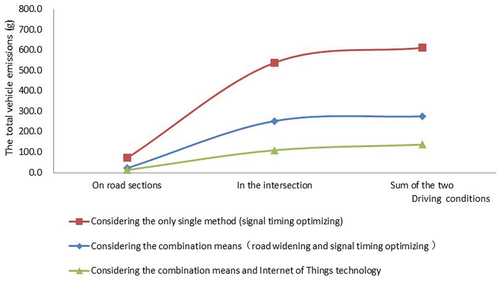
The trend of the total vehicle emissions and the total cost in the IoT environment is shown in Figure 6 at different values of $\mathit{c}{w}_2$. Figure 7 shows the trend of changes in total system impedance and total cost in the IoT environment at different values of $\mathit{c}{w}_2$. Comparison of vehicle emissions between the intersection and road sections at different values of cw2 is shown in Figure 8. Figure 9 depicts vehicle emissions comparison using different methods and IoT technology under the assumption that the condition ${\theta }_1:{\theta }_2:\mathit{c}{w}_2=1:1:1$.

Figure 6. The trend of the total vehicle emissions and the total cost in the IoT environment.

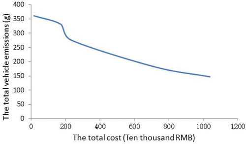
Figure 7. The trend of the total impedance and the total cost in the IoT environment.

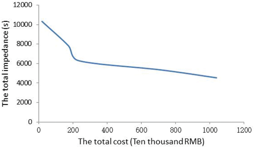
Figure 8. Comparison of vehicle emissions between the intersection and road sections.

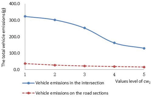
Figure 9. Comparison of vehicle emissions using different methods and IoT technology.

Analysis of Optimization Results

1. With the reduction of $\mathit{c}{w}_2$ in Figure 6, the trend correlates an increase in total cost with a reduction in the total amount of motor vehicle emissions reducing. This trend indicates that improving road capacity in the IoT environment can effectively reduce the total amount of motor vehicle emissions.

2. With the decrease in $\mathit{c}{w}_2$ in Figure 7, the increase in total cost associates with the system total impedance decreasing. This relationship indicates that improving the road capacity in the IoT environment can effectively reduce the total system impedance.

3. In Figure 8, the vehicle emissions at the intersection are much greater than the emissions on the road sections. Considering the only single method (signal timing optimizing), the difference between the two is about 7.4 times. Therefore, in order to alleviate the degree of urban traffic pollution, we must focus on how to reduce the idle pollution emissions of motor vehicles at the intersection.

4. In Figure 8, the total amount of vehicle emissions on the road section is maintained at a stable level. However, the vehicle emissions at the intersection are significantly reduced. This trend indicates that the increase in road widening and IoT technology investment can reduce the emissions at the intersections. However, improving the traffic conditions at intersections can greatly enhance traffic efficiency and alleviate exhaust emissions. Because the layout of the traffic infrastructure in intersections is limited by the number of lanes, land use pattern, and block buildings, the traffic management department cannot infinitely improve the traffic facilities at intersections.

5. In Figure 9, the total vehicle emissions by using the IoT technology is considered to be significantly smaller than that of using the only single method (such as signal timing optimization), and by comparison to other combination strategies (road widening and signal timing optimization). This observation demonstrates that the combination strategy in the IoT environment by moderately increasing supply and reasonable guidance of traffic demand can minimize vehicle emissions in urban road networks.

Sensitivity Analysis

Sensitivity analysis is a method used to evaluate the sensitivity of model output changes to parameter changes. Literature studies have shown that although the changes in the capacity increment of the road section are not obvious after considering vehicle emissions, the value of the objective function varies greatly (Yang and Su 2013). In the models proposed in the paper, the variables $\mathrm{c}{\mathrm{w}}_1$ and $\mathrm{c}{\mathrm{w}}_2$ have the greatest impact on the total target value. Therefore, sensitivity analysis is necessary to further analyze the impact of changes in the vehicle emissions conversion coefficient $\mathrm{c}{\mathrm{w}}_1$and the total cost conversion factor $\mathrm{c}{\mathrm{w}}_2$ on the decision value.

Combined with the case study, when the values of the vehicle emissions conversion coefficient cw1 and the total cost conversion factor $\mathit{c}{w}_2$ are different, the changing rule of the model decision value is conducive to guiding the road network design and planning more effectively. Using the IS-APCPSO algorithm to obtain the trend line for the decision value with respect to the conversion coefficient is shown in Figure 10.

Figure 10. Change of the decision value with the conversion factor.

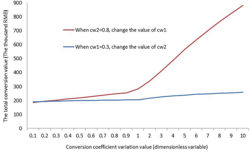
Figure 10 demonstrates that when the total cost conversion factor $\mathit{c}{w}_2$ remains unchanged at 0.8, the decision value rises quickly after the vehicle emissions conversion coefficient cw1 is slowly increased. By contrast, when the vehicle emissions coefficient $\mathit{c}{w}_1$ is kept constant at 0.3, the decision value displays minimal increases with little increase in the total cost conversion factor $\mathit{c}{w}_2$, and this relationship tends to be almost a straight line. This trend shows that the change of the vehicle emissions conversion coefficient cw1 has more influence on the change of the decision than the conversion factor $\mathit{c}{w}_2$ of the total cost.

The upper-level planning model is multi-objective in the design of a continuous transportation network, in order to minimize the weighted sum of total system impedance, vehicle emissions, and the total cost. However, the makers of these goals come from the traffic management department, the environmental protection department, and the investment department. On the premise of meeting a certain traffic volume, there is a contradiction between minimizing the total impedance and minimizing the cost of decision-makers. There may be conflicts and interests between them. Therefore, seeking reasonable weight among different goals is one of the important contents of sensitivity analysis.

When $\mathit{c}{w}_2$ = 0.8, the range of change of $\mathit{c}{w}_1$ is relatively large, which shows that vehicle emissions have a greater impact on the decision value. In essence, with the increasing emphasis on environmental protection and carbon neutrality, effective control of vehicle emissions in urban road networks is the key task. Therefore, the discussion of different situations is significant. If there is less traffic (in the flat peak period) of the road network, the balance between total system impedance and vehicle emissions should be sought. It is recommended that the parameter $\mathit{c}{w}_1$ should be bound between [0, 1]. If there is large traffic (in peak period of traffic or congested state) of the road network, the emphasis on the vehicle emissions should be increased. The implications of the model imply that cw1 can be set according to a certain ratio to the saturation of the road section.

When $\mathit{c}{w}_1=0.3$, $\mathit{c}{w}_2$ changes relatively smoothly, indicating that the impact of the total cost on the decision value is relatively small. The larger the $\mathit{c}{w}_2$, the more stressful it is on funds for road widening and IoT technology applications. The more restricted, the more attention will be given by the relevant departments when making decisions. The smaller the $\mathit{c}{w}_2$, the more abundant funds for road widening and IoT technology application. Based on our model findings, the recommendation is that the parameter $\mathit{c}{w}_2$ should be bound within the range [0, 1]. Based on this determination, a scenario application based on the parameters $\mathit{c}{w}_1$ and $\mathit{c}{w}_2$ is established. If the road network diagram of this example is a schematic diagram of a part of a road network in an underdeveloped area with severe traffic congestion, the model recommendation implies that $\mathit{c}{w}_1$ should be greater than 1. Additionally, $\mathit{c}{w}_2$ of approximately 1 is more appropriate.

Conclusions and Future Work

Conclusions

On the basis of discussing motor vehicle pollution emission control, a bi-level programming model of traffic flow control and exhaust emission control in IoT is proposed in the paper. The validity of the model and the algorithm is demonstrated using a typical case. First of all, the application of IoT to fixed road sections, intersections, vehicles, and communication terminal can produce a wider range of data collection and higher precision reading. Second, the real-time collection or transmission of images, videos, and other data can be achieved more precisely by using sensors and specialized equipment of IoT. Third, the data information transmitted in IoT is more accurate and reliable, such as traffic flow, vehicle speed, air quality, noise levels, and other indicators. Fourth, IoT data can be more integrated with other data sources such as traffic cameras, social media, mobile applications, and intelligent driving, which contribute to the integration and improvement of data, thus providing decision-makers with more comprehensive and accurate auxiliary support.

The achievements of this research manuscript include:

1. A novel mathematical model and multi-objective method are presented for reducing vehicle emissions with the combination of traditional tools and IoT technologies. The application of IoT mainly includes RFID, MEMS, automatic recognition technology, sensor network technology, and positioning technology to achieve real-time and comprehensive collection of traffic information resources, and ensure the real-time, complete, consistent, and accurate collection of traffic data (including images and videos). The novel multi-objective model is more in line with the actual situation of urban traffic network, and the urban road traffic system optimization by utilizing IoT technology is more effective in reducing total impedance and reducing vehicle emissions.

2. A cost model for IoT technology in urban road networks is established, and an IS-APCPSO algorithm for solving the complex integration model is designed. The use of IoT requires funding from public or private. The investment cost of IoT includes the construction cost of IoT infrastructure, research costs, and daily maintenance of IoT. According to the analysis in the paper, if the cost of using the IoT can be controlled at a certain level, it is beneficial for urban road traffic optimization. On the contrary, further improvement is needed. Taking into account the investment cost of IoT technology in the multi-objective models can more accurately reflect the importance of new technology investment, making it easier to adopt the suggestions of this paper for urban traffic management departments.

3. Based on the discharge rate and emission factors as a function of the relevant variables, the corresponding idling rate model and uniform emission factor model are developed in the paper. Considering different driving conditions, a vehicle emission factor prediction model using IoT technology can more accurately reflect the actual vehicle emissions in the urban road traffic system. Moreover, the emission rate model with sub-idle time is more scientific and reasonable, which is more consistent with actual vehicle emission patterns.

4. Sensitivity analysis of the model enhances the practical application of the proposed model in reflecting the characteristics of economic development in each region and the differentiated traffic conditions. Comparing the changes in road network impedance and vehicle emissions before and after using IoT technology, it can be concluded that using IoT technology traffic guidance is beneficial for traffic management departments by using IoT to adopt collaborative strategies and improve traffic conditions (alleviate traffic congestion and reduce exhaust emissions). This conclusion is similar to the research findings of some scholars (Ye 2015).

Meanwhile, the models and IS-APCSO algorithm proposed in this paper have limitations. The influence of factors on exhaust emissions also includes motor vehicle type and engine condition, whether conditions and road slope. New energy vehicles are gradually increasing in many metropolises (no exhaust emissions to the new energy, but the impact on road impedance is visible), and the solution of the algorithm still needs further improvement. Although the IS-APCPSO proposed can improve previous algorithm performance, it is prone to premature convergence and falling into local extremes due to poor local search ability and lack of search diversity. Moreover, as mentioned in the previous model construction and case analysis, in order to simplify the model and facilitate calculation, we only selected a small number of variables and estimated some parameters based on previous research results. These will have a significant impact on the optimization results, and take new traffic management measures in actual urban road traffic system.

We employed a simplified urban road network and fixed vehicle travel routes, which are indeed different from real-world traffic. On the one hand, the typical case is beneficial for comparing with previous research results. On the other hand, more complex urban road traffic networks require more advanced computing hardware and software to solve large-scale problems. This is also a new research challenge that can be considered as one of the subsequent research topics. It should be noted that different urban road traffic conditions (such as interference between vehicles and non-vehicles, lane width, traffic density, and central median) have a significant impact on driving speed and vehicle emissions on urban roads. However, the premise of this research is to demonstrate whether the application of IoT technology can improve road operation efficiency and thereby reduce total vehicle emissions under the same urban road traffic conditions. As for the impact of different urban road traffic conditions on the models, we can improve it in subsequent research. In addition, there are many challenges in the application of IOT in urban traffic management, such as personal privacy protection, driver interference and safe driving, IoT standards and compatibility, multi-scenario application, and emergency response.

Future Work

Optimizing urban road traffic systems utilizing IoT technology still faces many challenges and issues, such as network security, data collection strategies, data privacy protection, multi-system integration, and standardization. Therefore, we should increase the importance of network security, privacy protection and standardization to ensure the operation of IoT. In addition, the policy supporting and legal protection the promotion are also important for the promotion of IoT technology in urban road network. Future research is possible in a number of areas. Some research shortcomings of this paper and future research areas are emphasized as follows. First, in order to avoid subjective randomness in parameter selection, sensitivity analysis of influence factor such as the weight coefficient can be used as one of the directions for further improvement research. We also need to analyze other factors that affect urban road traffic impedance, total cost, and exhaust emissions, as well as the correlation between each factor. The value of weights is also related to the preferences of urban traffic management departments for different objectives. This is a complex decision-making process that requires further research and continuous practical application. Second, the regional signal linkage control, vehicle acceleration and deceleration, and effects of different vehicles pollution should be considered with cloud computing and big data technologies. The above involves how to achieve data compatibility and multi-scenario applications between IOT and other intelligent systems. Third, further study should address the impact of IoT implementation on traffic flow, idle time, and the impedance function. We can also research on the specific applications of RFID, sensor detection, accident prediction and processing, and parking management in the IoT. Fourth, we should also pay attention to the challenges faced by the application of IoT in urban traffic systems, such as data privacy, moral ethics, systemic security (such as hacker attacks), and international standards. Finally, more urban road network design examples or the selection of some regional aspects in metropolis should be applied, in order to verify the effectiveness of the models and algorithms. In the future, we can use different operational data from time periods, road networks, and actual roads to calibrate parameters of the models, and to further analyze the simulation results. Then, we can objectively select model variables and determine parameter values to improve models and algorithms proposed in this paper by comparing multiple case studies.

Disclosure Statement

No potential conflict of interest was reported by the author(s).

Data availability statement

The data that support the findings of this study are available from the corresponding author upon reasonable request.

Supplementary Material

Supplemental data for this article can be accessed online at https://doi.org/10.1080/08839514.2024.2344144

Additional information

Funding

This work was supported by the Zhejiang Province Social Science Foundation under Grant [21NDJC182YB].

Notes on contributors

Ke Huang

Ke Huang is an associate professor at the School of Information and Electrical Engineering in Hangzhou City University. She is mainly engaged in traffic optimization design, intelligent transportation, automatic driving, logistics innovation management, and other related research fields. She has presided over more than 20 scientific research projects and published more than 30 academic papers.

Jianjun Zhu

Jianjun Zhu graduated from the School of Transportation & Logistics in Southwest Jiaotong University, China, with a doctor’s degree in 2011. He is mainly engaged in comprehensive transportation, financial engineering, and economic management. He has chaired over more than 10 high-level scientific research projects and has published more than 20 academic papers.

References

- Antonio, P., G. Claudio, M. Eloísa, F. Paulo. 2023. Road traffic noise monitoring in a Smart City: Sensor and Model-Based approach. Transportation Research Part D: Transport and Environment 125. doi:10.1016/j.trd.2023.103979.
- Asma, A. O., B. Ayoub, B. Assia, and T. Mohamed. 2022. Overview of Road Traffic Management Solutions based on IoT and AI. Procedia Computer Science 198:518–32. doi:10.1016/j.procs.2021.12.279.
- Bhavana, P., P. Likhitha, C. Manoj, and L. S. Kumar. 2023. IoT based Dynamic Road Traffic Management System. Journal of Physics: Conference Series 2466 (1). doi: 10.1088/1742-6596/2466/1/012025.
- Chen, J., Z. Y. Mei, and W. Wang. 2007. Road resistance model under mixed traffic flow conditions with curb parking. China Civil Engineering Journal 40 (9):95–100.
- Chen, K., and Y. U. Lei. 2007. Microscopic traffic-emission simulation and case study for evaluation of traffic control strategies. Journal of Transportation Systems Engineering & Information Technology 7 (1):93–99. doi:10.1016/S1570-6672(07)60011-7.
- Coensel, B. D., A. Can, B. Degraeuwe, I. D. Vlieger, and D. Botteldooren. 2011. Effects of traffic signal coordination on noise and air pollutant emissions. Environmental Modelling & Software 35 (4):74–83. doi:10.1016/J.ENVSOFT.2012.02.009.
- Darwish, R. R. 2022. A congestion-aware decision-driven architecture for information-centric Internet-of-Things applications. International Journal of Computers and Applications 44 (4):324–37. doi:10.1080/1206212X.2020.1738088.
- Dipti, M., and S. Abhijit. 2022. IoT-based air pollution detection, monitoring and controlling system. Journal of Discrete Mathematical Sciences and Cryptography 25 (7):2173–82. doi:10.1080/09720529.2022.2133254.
- Gao, Z. Y., and Y. F. Song. 2002. A reserve capacity model of optimal signal control with user-equilibrium route choice. Transportation Research Part B 36 (4):313–23. doi:10.1016/S0191-2615(01)00005-4.
- Gao, Z. Y., Y. F. Song, and B. F. Si 2000. Urban traffic continuously balanced network design: Theory and method. China Railway Press, Beijing, China.
- Gong, J. 2011. Effect analysis and optimizing control of bus operation. Ph.D. dissertation, Wuhan University of Technology, Wuhan, China.
- Guerrero, I. J., S. Zeadally, and C. J. Contreras. 2015. Integration challenges of intelligent transportation systems with connected vehicle, cloud computing, and internet of things technologies. IEEE Wireless Communications 22 (6):122–28. doi:10.1109/MWC.2015.7368833.
- Hepsiba, D., L. M. Varalakshmi, M. S. Kumar. 2021. Automatic pollution sensing and control for vehicles using IoT technology. Materials Today 45(2).
- Huang, K. 2011. Optimization model and algorithm of urban traffic network considering environmental pollution control. Ph.D. dissertation, Southwest Jiaotong University, Chengdu, China.
- Huang, K., H. L. Zhang, Y. W. Wang, and C. B. Yu 2017. An improved adaptive propagation chaotic particle swarm optimization algorithm based on immune selection. Proceedings of the 2017 International Conference on Machine Learning and Cybernetics (ICMLC 2017), Ningbo, China, 105–10.
- Huang, K., H. L. Zhang, and G. L. Yang. 2019. An optimized IS-APCPSO algorithm for large scale complex traffic network. CLUSTER COMPUTING-THE JOURNAL OF NETWORKS SOFTWARE TOOLS AND APPLICATIONS 22 (2):3271–84. doi:10.1007/s10586-018-2082-6.
- Kwak, J., B. Park, and J. Lee. 2011. Evaluating the impacts of urban corridor traffic signal optimization on vehicle emissions and fuel consumption. Transportation Planning and Technology 35 (2):145–60. doi:10.1080/03081060.2011.651877.
- Liu, C., and L. Ke. 2023. Cloud assisted Internet of things intelligent transportation system and the traffic control system in the smart city. Journal of Control and Decision 10 (2):174–87. doi:10.1080/23307706.2021.2024460.
- Liu, S. D., Y. Qi, C. G. Tan, and H. R. Liu. 2017. Plug-in hybrid electric vehicle (PHEV) energy management strategy based on improved chaotic particle swarm optimization (ICPSO). Automobile Applied Technology 17:78–80.
- Nagurney, A., and J. Dong. 2002. A multiclass multicriteria traffic network equilibrium model with elastic demand. Transportation Research B 36 (5):445–69. doi:10.1016/S0191-2615(01)00013-3.
- Noland, P. B. 2001. Relationships between highway capacity and induced vehicle travel. Transportation Research Part A 35 (1):47–72. doi:10.1016/S0965-8564(99)00047-6.
- Palconit, M. G., and W. A. Nuez 2017. CO2 emission monitoring and evaluation of public utility vehicles based on road grade and driving patterns: An Internet of Things application. 9th IEEE International Conference on Humanoid, Nanotechnology, Information Technology, Communication and Control, Environment and Management (IEEE HNICEM), Pasay, Philippines. doi:10.1109/HNICEM.2017.8269496.
- Pampa, S., and G. Firoj 2018. An IoT based Intelligent Traffic Congestion Control System for Road Crossings. International Conference on Communication, Computing and Internet of Things (IC3IoT), Chennai, India. doi: 10.1109/IC3IoT.2018.8668131.
- Pankaj, P. T., D. G. Rahul, and K. G. Pradeep. 2023. An IoT-based framework of vehicle accident detection for smart city. IETE Journal of Research 8):1-14. doi:10.1080/03772063.2023.2239757.
- Park, B., I. Yun, and K. Ahn. 2009. Stochastic optimization for sustainable traffic signal control. International Journal of Sustainable Transportation 3 (4):263–84. doi:10.1080/15568310802091053.
- Peng, H. Q., W. Xie, and X. You. 1997. Research on conversion methods of highway transportation volume and traffic volume. Inner Mongolia Highway and Transport 3 (2):36–38.
- Rakha, H., and K. Ann. 2004. Integration modeling framework for estimating mobile source emissions. Journal of Transportation Engineering 130 (2):183–93. doi:10.1061/(ASCE)0733-947X.
- Ren, G. 2007. Traffic assignment model and algorithm under traffic management measures. Nanjing, China: Southeast University Press.
- Sarkar, S., S. Chatterjee, and S. Misra. 2018. Assessment of the suitability of fog computing in the context of internet of things. IEEE Transactions on Cloud Computing 6 (1):46–59. doi:10.1109/TCC.2015.2485206.
- Sha, X. F. 2007. Research on vehicle dynamic emission model on urban road. Ph.D. dissertation, Jilin University, Jilin, China.
- Shen, Y., T. R. Wu, J. Yan. 2021. Investigation on air pollutants and carbon dioxide emissions from motor vehicles in Beijing based on COPERT models. Journal of Environmental Engineering Technology 11 (6):1075–82.
- Shi, Y. H., and R. C. Eberhart 1998. Parameter selection in particle swarm optimization. Proceeding of 1998 Annual Conference on Evolutionary Programming. San Diego: Springer-Berlin, USA:591-600. doi:10.1007/BFb0040810.
- Stevanovic, A., P. Martin, and J. Stevanovic. 2007. VISSIM-based genetic algorithm optimization of signal timings. Transportation Research Record: Journal of the Transportation Research Board 2035 (1):59–68. doi:10.3141/2035-07.
- Su, M. W. 2015. Theoretical analysis and countermeasures research on the development of internet of things industry. Ph.D. dissertation, JiLin, University, Changchun, China.
- Sun, D. Z. 2010. Urban traffic road environmental air quality testing and evaluation. Beijing, China: China Environmental Science Press.
- Sun, Q. B., J. Liu, S. Li, C. X. Fan, and J. J. Sun. 2010. Internet of things: Summarize on concepts, architecture and key technology problem. Journal of Beijing University of Posts and Telecommunications 33 (3):1–9.
- Sun, W., A. Vij, N. Kaliszewski, and J. J. M Rose., 2023. A flexible and scalable single-level framework for OD matrix inference using IoT data. Transportation Research Part A: Policy and Practice 175:1–12. doi:10.1016/j.tra.2023.103775.
- Tu, D. F., E. L. Wang, F. Zhang, and H. F. Xu. 2017. Research on vehicle exhaust dynamic monitoring system based on Internet of Things. Journal of Chifeng University(Natural Science Edition) 33 (24):30–31.
- Vimal, K. D., R. Bhuvaneshwari, M. Pooja. 2022. IOT based vehicle emission monitoring system and pollution detection. International Journal of Advanced Research in Science, Communication and Technology 343–49. doi:10.48175/IJARSCT-3271.
- Vong, C. M., P. K. Wong, Z. Q. Ma, and K. I. Wong. 2014. Application of RFID technology and the maximum spanning tree algorithm for solving vehicle emissions in cities on internet of things. Internet of Things, IEEE 26 (1):347–52.
- Wang, X. H., and H. Du. 2016. Cold chain logistics decision-making of fresh agricultural products based on the internet of things adoption: From the perspective of cost-benefit. Systems Engineering 34 (6):89–97.
- Wang, X. W., T. Z. Li, L. Wang, B. Li, and W. He. 2010. Environmental traffic impedance model of street canyon based on health impacts. Journal of Southeast University (Natural Science Edition) 40 (1):196–200. doi:10.3969/j.1001-0505.2010.01.037.
- Wei, L. 2011. A simulation and optimization study of urban road traffic emissions. Ph.D. dissertation, Wuhan University of Technology, Wuhan, China.
- Wu, L., P. J. Shao, and X. Yao. 2011. A comparative analysis based on PLM return model with internet of things to collect information. Systems Engineering 29 (6):86–93.
- Xiu, W. J., L. L. Zhang, K. L. Li, and M. Y. Wang. 2016. Intersection signal timing optimization control based on vehicle emission. Transport Research 2 (2):6–11.
- Xu, W., M. C. Fan, and H. L. Xu. 2016. Road pricing for a multi-modal transportation network with emission considerations. Systems Engineering—Theory & Practice 36 (9):2345–54. doi:10.12011/1000-6788.
- Xu, Y. F., L. Yu, and G. H. Song. 2016. GA-based approach to modeling operating mode distributions and estimating emissions. China Environmental Science 36 (12):3548–59.
- Yang, M., and B. Su. 2013. A model of continuous transportation network design based on cyclic economy and sensitivity analysis. Journal of Highway and Transportation Research and Development 30 (4):94–100.
- Yang, Y. N. 2014. Research on the design methodology of traffic management measures to reduce vehicular emissions. Ph.D. dissertation, Tsinghua University, Beijing, China.
- Yang, Z. S., C. Y. Lin, and B. Gong. 2009. Traffic signal cycle optimization. Traffic Information and Security 27 (3):35–38. doi:10.3963/j.cn.42-1781.U.2009.03.010.
- Ye, X. 2013. On the urban traffic guidance by the internet of things technology. In Master, dissertation. Chengdu, China: Southwest Jiaotong University.
- Yin, H. L. 2002. Urban traffic management planning theory system and key issues. Ph.D. dissertation, Southeast University, Nanjing, China.
- Yu, L., T. Wan, and X. M. Chen. 2008. Simulation study on traffic signal timing optimization integrating environmental factor and delay. Journal of System Simulation 20 (11):3016–31. doi:10.3724/SP.J.1077.2008.00933.
- Zhang, H., Z. Y. Gao, and B. Zhang. 2006. Model and algorithm of transportation network design for emission reduction. China Civil Engineering Journal 39 (11):114–19. doi:10.1016/S1872-2040(06)60039-X.
- Zhang, K., Y. J. Zhang, Y. He. 2016. Quantitative analysis of NO and NO2 from vehicle exhaust emission based on fast ICA and ANN. Journal of Atmospheric and Environmental Optics 11 (6):435–411.
- Zhang, X., H. D. Zhao, and D. J. Zhao. 2015. Automatic approach to develop driving cycles for estimation of vehicle emissions. Journal of Chongqing University 38 (3):28–38.
- Zhao, T., T. D. Guo, and Z. Y. Gao. 2005. A Optimal Model And Solution Algorithm For Maximal OD Travel Demand In Urban Transport Discrete Network Design Problem Under Environment Objective. China Civil Engineering Journal 38 (3):119–24.
- Zhou, S. P. 2009. Research on traffic signal control strategies in urban intersections based on emission factors. Ph.D. dissertation, Wuhan University of Technology, Wuhan, China. doi:10.7666/d.y1559709.
- Zou, Z. Y. 2009. Analysis of urban road network operation reliability and optimization. Ph.D. dissertation, Beijing Jiaotong University, Beijing, China. doi:10.7666/d.y1578666.