Handling Imbalanced Classification Problems by Weighted Generalization Memorization Machine

ABSTRACT

Imbalanced classification problems are of great significance in life, and there have been many methods to deal with them, e.g. eXtreme Gradient Boosting (XGBoost), Logistic Regression (LR), Decision Trees (DT), and Support Vector Machine (SVM). Recently, a novel Generalization-Memorization Machine (GMM) was proposed to maintain good generalization ability with zero empirical for binary classification. This paper proposes a Weighted Generalization Memorization Machine (WGMM) for imbalanced classification. By improving the memory cost function and memory influence function of GMM, our WGMM also maintains zero empirical risk with well generalization ability for imbalanced classification learning. The new adaptive memory influence function in our WGMM achieves that samples are described individually and not affected by other training samples from different category. We conduct experiments on 31 datasets and compare the WGMM with some other classification methods. The results exhibit the effectiveness of the WGMM.

Introduction

Imbalanced classification problems often prioritize the minority class, which typically holds more crucial information. Numerous real-world applications encounter imbalanced scenarios, including but not limited to network intrusion detection (Chen et al. 2022), cancer detection (Lilhore et al. 2022; Seo et al. 2022), mineral exploration (Xiong and Zuo 2020), illegal credit card transactions (Sudha and Akila 2021), bank fraud detection (Abdelhamid, Khaoula, and Atika 2014), and Advertisement click-through rate prediction (Zhang, Fu, and Xiao 2017). Two main categories of methods are used to address imbalanced classification problems. The first category, known as data-level methods, focuses on transforming imbalanced data into balanced data. This includes oversampling methods (Chawla et al. 2002; He and Garcia 2009; He et al. 2008; Nguyen, Cooper, and Kamei 2011; Zheng 2020); and undersampling methods (Hart 1968; Sui, Wei, and Zhao 2015). The second category, algorithm-level methods, adjusts the weights of majority and minority classes within models. Examples include cost-sensitive methods (Bach, Heckerman, and Horvitz 2006), kernel adaptation methods (Mathew et al. 2017), and hyperplane shifting methods (Datta and Das 2015). Including methods such as Logistic Regression (LR) (Luo et al. 2019), Cost-Sensitive Decision Trees (Krawczyk, Woźniak, and Schaefer 2014), Cost-Sensitive Neural Networks (Krawczyk and Woźniak 2015) and Support Vector Machine (SVM), among which the support vector machine algorithm is better at solving imbalanced problems due to the strong generalization ability of SVM.

The SVM, by minimizing the sum of empirical and expected risks, has found extensively used in practical real-world applications, including face recognition (Chaabane et al. 2022), cancer detection (Alfian et al. 2022; Hussain et al. 2011; Seo et al. 2022); voice recognition (Harvianto et al. 2016) and handwritten character recognition (Hamdan and Sathesh 2021; Kibria et al. 2020; Kumar, Sharma, and Jindal 2011; Nasien, Haron, and Yuhaniz 2010). However, the classic SVM cannot always guarantee zero empirical risk, which classifies all training samples correctly. For the SVM, Vapnik proposed a generalization-memorization kernel (Vapnik and Izmailov 2021) to correctly classify training samples and have good generalization ability. Subsequently, a generalization-memorization machine (GMM) (Wang and Shao 2022) was proposed to account for the mechanism of the generalization-memorization kernel. The GMM enhances memorization by incorporating a memory cost function and improves generalization through a memory influence function. Since the memory influence function is predefined uniformly on the training set, the inessential samples would obtain some larger effects on prediction, especially for imbalance problems.

In this paper, we propose a Weighted Generalization Memorization Machine (WGMM) to deal with the imbalanced classification problem. Our WGMM employs distinct memory cost functions for the majority and minority classes. While preserves zero empirical risk. Furthermore, our WGMM also introduces a self-adaptive memory influence function to adapt to various imbalance problems.

The structure of this paper is as follows: In the next section, a brief overview of GMM and imbalanced classification methods is given. The third part establishes our WGMM model. The last two sections present numerical experiments and conclusions.

Related Works

Imbalanced Classification

There are two primary approaches to deal with imbalanced classification problems: data-level (DL) preprocessing methods (Chawla et al. 2002; Hart 1968; He and Garcia 2009; He et al. 2008; Nguyen, Cooper, and Kamei 2011; Sui, Wei, and Zhao 2015; Zheng 2020) and algorithm-level (AL) methods (Bach, Heckerman, and Horvitz 2006; Batuwita and Palade 2010; Datta and Das 2015; Imam, Ting, and Kamruzzaman 2006; Iranmehr, Masnadi-Shirazi, and Vasconcelos 2019; Mathew et al. 2017). Data-level preprocessing methods aim to mitigate class imbalance by adjusting the training data through sample addition or removal to achieve class balance before model training. The oversampling or undersampling is always concerned. Thereinto, oversampling methods rebalance classes by either replicating or generating samples within the minority class. For instance, Random oversampling (ROS) (He and Garcia 2009) involves duplicating samples from the minority class, while Synthetic Minority Over-sampling Technique (SMOTE) (Chawla et al. 2002) generates artificial samples to balance the training data by linearly interpolating samples from the minority class. Furthermore, other SMOTE variants exist, such as SVM-SMOTE (Nguyen, Cooper, and Kamei 2011), Borderline-SMOTE (Zheng 2020), Kmeans-SMOTE (Zheng 2020) and ADASYN (He et al. 2008). Undersampling methods balance the dataset by removing instances from the majority class. For instance, Random undersampling (RUS) (Sui, Wei, and Zhao 2015) entails the random removal of instances from the majority class until a specified class balance is achieved.

Algorithm level methods aim to construct a particular classifier to handle imbalanced classification problems. There have been many approaches based on this strategy, such as Fuzzy Support Vector Machines for Class Imbalance Learning (FSVM-CIL) (Batuwita and Palade 2010), Cost-sensitive support vector machines (CSSVM) (Iranmehr, Masnadi-Shirazi, and Vasconcelos 2019) and z-SVM (Imam, Ting, and Kamruzzaman 2006). Introducing fuzzy membership values enables FSVM-CIL to prioritize the minority class while accounting for the majority class, resulting in improved performance on imbalanced datasets. CSSVM assigns distinct misclassification costs to various classes, with a primary focus on prioritizing minority classes. z-SVM embraces a cost-sensitive approach, where it assigns class-specific costs to misclassifications, offering significant value when a class is rare or holds greater importance.

Generalization-Memorization Machine

Recently, the generalization-memorization machine (GMM), the SVM with a new memory mechanism, have been proposed for classification in the n-dimensional real space ${\mathbb{R}}^n$. Suppose $\mathbf{T}=\{({\mathbf{x}}_i,y_i)|\mathit{i}=1,2,\dots ,\mathit{m}\}$ is the training set, where ${\mathbf{x}}_i\in {\mathbb{R}}^n$ is the input sample, and $y_i=\{+1,-1\}$ is the corresponding output. We organize the training set into $\mathbf{X}$ and $\mathbf{Y}$, where $\mathbf{X}\in {\mathbb{R}}^{\mathit{n}\text{timesm}}$ is the sample matrix composed of ${\mathbf{x}}_i$, $\mathbf{Y}$ is a diagonal matrix composed of labels, and the element on the diagonal is ${\mathbf{Y}}_{\mathit{ii}}=y_i$ with $\mathit{i}=1,2,\dots ,\mathit{m}$.

GMM considers the optimization problem as

(1) $\begin{array}{cc}\underset{\mathbf{w},b,\mathbf{c},d_{\cdot }}{\min }& \frac{1}{2}\parallel \mathbf{w}{\parallel }^2+\frac{\lambda }{2}\parallel \mathbf{c}{\parallel }^2+\mathit{C}\sum _{\mathit{i}=1}^m{d}_i\\ \mathrm{s}.\mathrm{t}.& y_i(\mathit{\phi }{({\mathbf{x}}_i)}^{\mathrm{T}}\mathbf{w}+\mathit{b}+\sum _{\mathit{j}=1}^m{y}_j{c}_j\mathit{\delta }({\mathbf{x}}_i,{\mathbf{x}}_j))\ge 1-d_i,\\ \mathit{\hspace{0.17em}}& d_i\ge 0,\mathit{i}=1,\dots ,\mathit{m},\end{array}$(1)

where $\parallel \cdot \parallel$ is ${\mathrm{L}}_2$ norm, $\mathit{\phi }(\cdot )$ is a mapping, $\mathit{\lambda }$ and $\mathit{C}$ are positive parameters, and $d_i$ is a slack variable. $\mathbf{c}$ is a column vector composed of $c_j(\mathit{j}=1,\dots ,\mathit{m})$, which is called memory cost and $\mathit{\delta }({\mathbf{x}}_i,{\mathbf{x}}_j)$ is called memory impact of ${\mathbf{x}}_j$ on ${\mathbf{x}}_i$.

The goal of this optimization problem is to find a hyperplane that correctly classifies the training datasets and has the largest margin. The first term $\frac{1}{2}\parallel \mathbf{w}{\parallel }^2$ is half the square of the margin, and by minimizing this term we are trying to maximize the margin. The second term $\frac{\lambda }{2}\parallel \mathbf{c}{\parallel }^2$ is the regularization term of the memory cost function, where $\mathit{\lambda }$ control the minimization of the sample memory cost function. Increasing $\mathit{\lambda }$ will increase the penalty on memory cost, thus placing more emphasis on classification accuracy. $\mathit{C}\sum _{\mathit{i}=1}^m{d}_i$ is the minimum training sample re-memory terms. In this way, the goal is to control the size and complexity of the model. $y_i(\mathit{\phi }({\mathbf{x}}_i{)}^{\mathrm{T}}\mathbf{w}+\mathit{b}+\sum _{\mathit{j}=1}^m{y}_j{c}_j\mathit{\delta }({\mathbf{x}}_i,{\mathbf{x}}_j))\ge 1-d_i$ is established indicating that each training sample is correctly classified.

For a new sample $\mathbf{x}$, outside the training set, it would be classified into positive class if $\mathit{\phi }({\mathbf{x}}_i{)}^{\mathrm{T}}\mathbf{w}+\mathit{b}+\sum _{\mathit{j}=1}^m{y}_j\mathit{c}({\mathbf{x}}_j)\mathit{\delta }({\mathbf{x}}_i,{\mathbf{x}}_j)>0$, and otherwise, it is classified into the negative class.

GMM has been proved that it could obtain zero empirical risk, and its classification performance in numerical experiments is much higher than the SVMs.

Weighted Generalization Memorization Machine (WGMM)

Building upon the foundation of retaining all training samples, one of the advantages of GMM is that it can achieve superior test accuracy than SVM. However, GMM remains susceptible to issues related to sample imbalance. To mitigate this, we have enhanced GMM by optimizing both the memory cost function and the memory influence function, resulting in the development of our WGMM.

Model Formation

We introduce a weighted memory cost function component into the original objective function, with the objective of capturing distinct costs associated with various samples.

The training set includes a positive sample set ${\mathbf{T}}_1=\{({\mathbf{x}}_i,y_i)|\mathit{i}=1,2,\dots ,\mathit{p}\}$ and a negative sample set ${\mathbf{T}}_2=\{({\mathbf{x}}_k,y_k)|\mathit{k}=1,2,\dots ,\mathit{q}\}$ with $\mathit{p}+\mathit{q}=\mathit{m}$. Without loss of generality, consider the positive samples as the minority categories within the imbalanced dataset, with the assumption that the positive sample set ${\mathbf{X}}_1$ represents the minority class and the negative class sample set ${\mathbf{X}}_2$ represents the majority class, where ${\mathbf{X}}_1\in {\mathbb{R}}^{\mathit{n}\times \mathit{p}}$ and ${\mathbf{X}}_2\in {\mathbb{R}}^{\mathit{n}\times \mathit{q}}$ represent sample matrix composed of ${\mathbf{x}}_i$.

The optimization problem of WGMM can be expressed as follows:

(2) $\begin{array}{cc}\underset{\mathbf{w},b,\mathbf{c},d_{\cdot }}{\min }& \frac{1}{2}\parallel \mathbf{w}{\parallel }^2+\frac{{\lambda }_1}{2}\parallel {\mathbf{c}}_1{\parallel }^2+\frac{{\lambda }_2}{2}\parallel {\mathbf{c}}_2{\parallel }^2+{\lambda }_3\sum _{\mathit{i}=1}^p{d}_i+{\lambda }_4\sum _{\mathit{k}=1}^q{d}_k\\ \mathrm{s}.\mathrm{t}.& y_i(\mathit{\phi }{({\mathbf{x}}_i)}^{\mathrm{T}}\mathbf{w}+\mathit{b}+\sum _{\mathit{j}=1}^m{y}_j{c}_j\mathit{\delta }({\mathbf{x}}_i,{\mathbf{x}}_j))\ge 1-d_i,\\ \mathit{\hspace{0.17em}}& y_k(\mathit{\phi }{({\mathbf{x}}_k)}^{\mathrm{T}}\mathbf{w}+\mathit{b}+\sum _{\mathit{j}=1}^m{y}_j{c}_j\mathit{\delta }({\mathbf{x}}_k,{\mathbf{x}}_j))\ge 1-d_k,\\ \mathit{\hspace{0.17em}}& d_i\ge 0,\mathit{i}=1,\dots ,\mathit{p},\\ \mathit{\hspace{0.17em}}& d_k\ge 0,\mathit{k}=1,\dots ,\mathit{q},\end{array}$(2)

where ${\lambda }_1$, ${\lambda }_2$, ${\lambda }_3$ and ${\lambda }_4$ are positive parameters, ${\mathbf{c}}_1$ and ${\mathbf{c}}_2$ represent the memory cost functions for remembering positive samples and negative samples, ${\mathbf{c}}_1$ is a column vector consisting of $c_i=\mathit{c}(x_i)(\mathit{i}=1,\dots ,\mathit{p})$, $c_i$ is the memory cost function of the $\mathit{i}$th positive sample, ${\mathbf{c}}_2$ is a column vector composed of $c_k=\mathit{c}(x_k)(\mathit{k}=1,\dots ,\mathit{q})$, $c_k$ is the memory cost function of the $\mathit{k}$th negative sample. $d_i=\mathit{d}(x_i)(\mathit{i}=1,\dots ,\mathit{p})$ is the memory cost function of the $\mathit{i}$th positive sample, $d_k=\mathit{d}(x_k)(\mathit{k}=1,\dots ,\mathit{q})$ is the memory cost function of the $\mathit{k}$th negative sample.

The objective of formula (2) seeks the large margin with memory costs as lower as possible, and it controls the complexity of the model meanwhile. According to the constraints of formula (2), the memory cost function is a variable, and the memory cost function is split into ${\mathbf{c}}_1$ and ${\mathbf{c}}_2$, and multiply them by different parameters. The constraints within the optimization problem are separately defined for the positive and negative classes, allowing for individual control over the memory costs of each class, thus reflecting the importance of each respective class. GMM requires the predefinition of the influence function $\mathit{\delta }({\mathbf{x}}_i,{\mathbf{x}}_j)(\mathit{i},\mathit{j}=1,\dots ,\mathit{p})$. Subsequently, this paper will introduce an adaptive influence function, in alignment with sample adaptation, which will be elaborated on in the following section. The retention of memory for all training samples becomes crucial in compliance with the constraints specified in formula (2).

The decision function of our WGMM is

(3) $\begin{array}{c}\mathit{g}(\mathbf{x})=\left\{\begin{array}{cc}\mathit{\phi }{(\mathbf{x})}^{\mathrm{T}}\mathbf{w}+\mathit{b}+\sum _{\mathit{j}=1}^m{y}_j{c}_j\mathit{\delta }({\mathbf{x}}_j,{\mathbf{x}}_i)+y_i{d}_i,& \mathrm{if}\mathbf{x}={\mathbf{x}}_i,\mathrm{\exists }{\mathbf{x}}_i\in \mathbf{X},\\ \mathit{\phi }{(\mathbf{x})}^{\mathrm{T}}\mathbf{w}+\mathit{b}+\sum _{\mathit{j}=1}^m{y}_j{c}_j\mathit{\delta }({\mathbf{x}}_j,{\mathbf{x}}_i),& \mathrm{otherwise}.\end{array}\right.\end{array}$(3)

Formula (3) defines the decision function as a piecewise function. the decision function is a piecewise function. When the input test sample belongs to the training sample, the model employs the first function to make decisions. $\sum _{\mathit{j}=1}^m{y}_j{c}_j\mathit{\delta }({\mathbf{x}}_j,{\mathbf{x}}_i)$ represents the comprehensive influence of memory training samples on predictions. The function $\mathit{\delta }$ impacts memory capacity of the model. So $y_i{d}_i$ denotes the item re-memorized for the sample, enhancing memory accuracy, thereby guaranteeing a training accuracy rate be 1. Conversely, when the input sample is not part of the training set, $d_i$ has no practical effect on $\mathbf{x}$. In such cases, the model utilizes the second function as the testing function.

We now delve into the dual problem associated with (2). The original problem (2) can be written in matrix form

(4) $\begin{array}{cc}\underset{\mathbf{w},b,\mathbf{c},d}{\min }& \frac{1}{2}\parallel \mathbf{w}{\parallel }^2+\frac{{\lambda }_1}{2}\parallel {\mathbf{c}}_1{\parallel }^2+\frac{{\lambda }_2}{2}\parallel {\mathbf{c}}_2{\parallel }^2+{\lambda }_3{\mathbf{e}}_1^{\mathrm{T}}{\mathbf{d}}_1+{\lambda }_4{\mathbf{e}}_2^{\mathrm{T}}{\mathbf{d}}_2\\ \mathrm{s}.\mathrm{t}.& \mathit{\phi }{({\mathbf{X}}_1)}^{\mathrm{T}}\mathbf{w}+\mathit{b}{\mathbf{e}}_1+{\mathbf{\Delta }}_{11}{\mathbf{c}}_1-{\mathbf{\Delta }}_{12}{\mathbf{c}}_2\ge {\mathbf{e}}_1-{\mathbf{d}}_1,\\ \mathit{\hspace{0.17em}}& -\mathit{\phi }{({\mathbf{X}}_2)}^{\mathrm{T}}\mathbf{w}-\mathit{b}{\mathbf{e}}_2-{\mathbf{\Delta }}_{21}{\mathbf{c}}_1+{\mathbf{\Delta }}_{22}{\mathbf{c}}_2\ge {\mathbf{e}}_2-{\mathbf{d}}_2,\\ \mathit{\hspace{0.17em}}& {\mathbf{d}}_1\ge \mathbf{0},\\ \mathit{\hspace{0.17em}}& {\mathbf{d}}_2\ge \mathbf{0},\end{array}$(4)

where ${\mathbf{d}}_1$ and ${\mathbf{d}}_2$ are the memory cost functions for remembering positive samples and negative samples, ${\mathbf{d}}_1$ is a column vector composed of $d_i$, ${\mathbf{d}}_2$ is a column vector composed of $d_k$, ${\mathbf{\Delta }}_{11}\in {\mathbb{R}}^{\mathit{p}\times \mathit{p}}$ with element $\mathit{\delta }({\mathbf{x}}_i,{\mathbf{x}}_j)(\mathit{i},\mathit{j}=1,\dots ,\mathit{p})$, ${\mathbf{\Delta }}_{12}\in {\mathbb{R}}^{\mathit{p}\times \mathit{q}}$, ${\mathbf{\Delta }}_{21}\in {\mathbb{R}}^{\mathit{q}\times \mathit{p}}$, ${\mathbf{\Delta }}_{22}\in {\mathbb{R}}^{\mathit{q}\times \mathit{q}}$ are defined similarly to ${\mathbf{\Delta }}_{11}$. ${\mathbf{e}}_1$ is a vector of one with an $\mathit{p}$ dimension, and $e_2$ is a vector of one with a $\mathit{q}$ dimension, and elements of ${\mathbf{e}}_1$ and ${\mathbf{e}}_2$ are all ones.

In order to solve optimization problem (4), take it as the original optimization problem and apply Lagrangian duality to obtain the optimal solution of the original problem. We construct a LaGrange function

(5) $\begin{array}{cc}\mathrm{L}& =\frac{1}{2}\parallel \mathbf{w}{\parallel }^2+\frac{{\lambda }_1}{2}\parallel {\mathbf{c}}_1{\parallel }^2+\frac{{\lambda }_2}{2}\parallel {\mathbf{c}}_2{\parallel }^2+{\lambda }_3{\mathbf{e}}_1^{\mathrm{T}}{\mathbf{d}}_1+{\lambda }_4{\mathbf{e}}_2^{\mathrm{T}}{\mathbf{d}}_2\\ \mathit{\hspace{0.17em}}& -{\alpha }^{\mathrm{T}}(\mathit{\phi }{({\mathbf{X}}_1)}^{\mathrm{T}}\mathbf{w}+\mathit{b}{\mathbf{e}}_1+{\mathbf{\Delta }}_{11}{\mathbf{c}}_1-{\mathbf{\Delta }}_{12}{\mathbf{c}}_2-{\mathbf{e}}_1+{\mathbf{d}}_1)\\ \mathit{\hspace{0.17em}}& +{\beta }^{\mathrm{T}}(\mathit{\phi }{({\mathbf{X}}_2)}^{\mathrm{T}}\mathbf{w}+\mathit{b}{\mathbf{e}}_2+{\mathbf{\Delta }}_{21}{\mathbf{c}}_1-{\mathbf{\Delta }}_{22}{\mathbf{c}}_2+{\mathbf{e}}_2-{\mathbf{d}}_2)\\ \mathit{\hspace{0.17em}}& +{{\mathit{\gamma }}_{\mathbf{1}}}^{\mathrm{T}}{\mathbf{d}}_1+{{\mathit{\gamma }}_{\mathbf{2}}}^{\mathrm{T}}{\mathbf{d}}_2.\end{array}$(5)

The LaGrange multiplier vectors $\mathit{\alpha }$, ${\gamma }_{\mathbf{1}}\in {\mathbb{R}}^p$ and $\mathit{\beta }$, ${\gamma }_{\mathbf{2}}\in {\mathbb{R}}^q$ are introduced for each inequality constraint. Next, we present the Karush–Kuhn–Tucker (KKT) conditions (Fletcher 2000) for (4). The partial derivatives of (5) with respect to variables $\mathbf{w}$, $\mathit{b}$, ${\mathbf{c}}_1$, ${\mathbf{c}}_2$ ${\mathbf{d}}_1$ and ${\mathbf{d}}_2$ are

(6) $\frac{\mathrm{\partial }\mathit{L}}{\mathrm{\partial }\mathbf{w}}=\mathbf{w}-\mathit{\phi }({\mathbf{X}}_1)\mathit{\alpha }+\mathit{\phi }({\mathbf{X}}_2)\mathit{\beta }=0,$(6)

(7) $\frac{\mathrm{\partial L}}{\mathrm{\partial b}}=-{\mathbf{e}}_1^{\mathrm{T}}\mathit{\alpha }+e_2^{\mathrm{T}}\mathit{\beta }=0,$(7)

(8) $\frac{\mathrm{\partial L}}{\mathrm{\partial }{\mathbf{c}}_1}={\lambda }_1{\mathbf{c}}_1-{\mathbf{\Delta }}_{11}^{\mathrm{T}}\mathit{\alpha }+{\mathbf{\Delta }}_{12}^{\mathrm{T}}\mathit{\beta }=0,$(8)

(9) $\frac{\mathrm{\partial L}}{\mathrm{\partial }{\mathbf{c}}_2}={\lambda }_1{\mathbf{c}}_2-{\mathbf{\Delta }}_{22}^{\mathrm{T}}\mathit{\beta }+{\mathbf{\Delta }}_{12}^{\mathrm{T}}\mathit{\alpha }=0,$(9)

(10) $\frac{\mathrm{\partial L}}{\mathrm{\partial }{\mathbf{d}}_1}={\lambda }_3{\mathbf{e}}_1-\mathit{\alpha }-{\gamma }_{\mathbf{1}}=0,$(10)

and

(11) $\frac{\mathrm{\partial }\mathit{L}}{\mathrm{\partial }{\mathbf{d}}_2}={\lambda }_4{\mathbf{e}}_2-\mathit{\beta }-{\gamma }_{\mathbf{2}}=0.$(11)

(6–11) are calculated mathematically to get

(12) $\mathbf{w}=\mathit{\phi }({\mathbf{X}}_1)\mathit{\alpha }-\mathit{\phi }({\mathbf{X}}_2)\mathit{\beta },$(12)

(13) ${\mathbf{c}}_1=\frac{1}{{\lambda }_1}({\mathbf{\Delta }}_{11}^{\mathrm{T}}\mathit{\alpha }-{\mathbf{\Delta }}_{21}^{\mathrm{T}}\mathit{\beta }),$(13)

(14) ${\mathbf{c}}_2=\frac{1}{{\lambda }_2}({\mathbf{\Delta }}_{22}^{\mathrm{T}}\mathit{\beta }-{\mathbf{\Delta }}_{12}^{\mathrm{T}}\mathit{\alpha }),$(14)

(15) ${\gamma }_{\mathbf{1}}={\lambda }_3{\mathbf{e}}_1-\mathit{\alpha }\ge 0,\mathit{\alpha }\le {\lambda }_3{\mathbf{e}}_1,\mathit{\alpha }={\lambda }_3{\mathbf{e}}_1-{\gamma }_{\mathbf{1}},$(15)

and

(16) ${\gamma }_{\mathbf{2}}={\lambda }_4{\mathbf{e}}_2-\mathit{\beta }\ge 0,\mathit{\beta }\le {\lambda }_4{\mathbf{e}}_2,\mathit{\beta }={\lambda }_4{\mathbf{e}}_2-{\gamma }_{\mathbf{1}}.$(16)

Substitute (12–16) into Equation (4)(4) $\begin{array}{cc}\underset{\mathbf{w},b,\mathbf{c},d}{\min }& \frac{1}{2}\parallel \mathbf{w}{\parallel }^2+\frac{{\lambda }_1}{2}\parallel {\mathbf{c}}_1{\parallel }^2+\frac{{\lambda }_2}{2}\parallel {\mathbf{c}}_2{\parallel }^2+{\lambda }_3{\mathbf{e}}_1^{\mathrm{T}}{\mathbf{d}}_1+{\lambda }_4{\mathbf{e}}_2^{\mathrm{T}}{\mathbf{d}}_2\\ \mathrm{s}.\mathrm{t}.& \mathit{\phi }{({\mathbf{X}}_1)}^{\mathrm{T}}\mathbf{w}+\mathit{b}{\mathbf{e}}_1+{\mathbf{\Delta }}_{11}{\mathbf{c}}_1-{\mathbf{\Delta }}_{12}{\mathbf{c}}_2\ge {\mathbf{e}}_1-{\mathbf{d}}_1,\\ \mathit{\hspace{0.17em}}& -\mathit{\phi }{({\mathbf{X}}_2)}^{\mathrm{T}}\mathbf{w}-\mathit{b}{\mathbf{e}}_2-{\mathbf{\Delta }}_{21}{\mathbf{c}}_1+{\mathbf{\Delta }}_{22}{\mathbf{c}}_2\ge {\mathbf{e}}_2-{\mathbf{d}}_2,\\ \mathit{\hspace{0.17em}}& {\mathbf{d}}_1\ge \mathbf{0},\\ \mathit{\hspace{0.17em}}& {\mathbf{d}}_2\ge \mathbf{0},\end{array}$(4) to get the dual problem

(17) $\begin{array}{cc}\underset{\mathit{\alpha },\mathbf{b}}{\min }& \frac{1}{2}{\alpha }^{\mathrm{T}}(\mathit{K}({\mathbf{X}}_1,{\mathbf{X}}_1)+\frac{1}{{\lambda }_1}{\mathbf{\Delta }}_{11}{\mathbf{\Delta }}_{11}^{\mathrm{T}}+\frac{1}{{\lambda }_2}{\mathbf{\Delta }}_{12}{\mathbf{\Delta }}_{12}^{\mathrm{T}})\mathit{\alpha }\\ \mathit{\hspace{0.17em}}& +\frac{1}{2}{\beta }^{\mathrm{T}}(\mathit{K}({\mathbf{X}}_2,{\mathbf{X}}_2)+\frac{1}{{\lambda }_1}{\mathbf{\Delta }}_{21}{\mathbf{\Delta }}_{21}^{\mathrm{T}}+\frac{1}{{\lambda }_2}{\mathbf{\Delta }}_{22}{\mathbf{\Delta }}_{22}^{\mathrm{T}})\mathit{\beta }\\ \mathit{\hspace{0.17em}}& -\frac{1}{2}{\alpha }^{\mathrm{T}}(\mathit{K}({\mathbf{X}}_1,{\mathbf{X}}_2)+\frac{1}{{\lambda }_1}{\mathbf{\Delta }}_{11}{\mathbf{\Delta }}_{21}^{\mathrm{T}}+\frac{1}{{\lambda }_2}{\mathbf{\Delta }}_{12}{\mathbf{\Delta }}_{22}^{\mathrm{T}})\mathit{\beta }\\ \mathit{\hspace{0.17em}}& -\frac{1}{2}{\beta }^{\mathrm{T}}(\mathit{K}({\mathbf{X}}_2,{\mathbf{X}}_1)+\frac{1}{{\lambda }_1}{\mathbf{\Delta }}_{21}{\mathbf{\Delta }}_{11}^{\mathrm{T}}+\frac{1}{{\lambda }_2}{\mathbf{\Delta }}_{22}{\mathbf{\Delta }}_{12}^{\mathrm{T}})\mathit{\alpha }\\ \mathit{\hspace{0.17em}}& -{\mathbf{e}}_1^{\mathrm{T}}\mathit{\alpha }-{\mathbf{e}}_2^{\mathrm{T}}\mathit{\beta }\\ \mathrm{s}.\mathrm{t}.& {\mathbf{e}}_1^{\mathrm{T}}\mathit{\alpha }-{\mathbf{e}}_2^{\mathrm{T}}\mathit{\beta }=0,\\ \mathit{\hspace{0.17em}}& \mathbf{0}\le \mathit{\alpha }\le {\lambda }_{\mathbf{3}}{\mathbf{e}}_{\mathbf{1}},\\ \mathit{\hspace{0.17em}}& \mathbf{0}\le \mathit{\beta }\le {\lambda }_{\mathbf{4}}{\mathbf{e}}_{\mathbf{2}},\end{array}$(17)

where $\mathit{K}(\cdot ,\cdot )$ represents a generalized Gaussian kernel with a parameter $\mathit{\sigma }$. Furthermore, when examining the solutions for $\mathit{\alpha }$ and $\mathit{\beta }$, where $\mathit{\alpha }$ has $\mathit{l}$ non-zero components and $\mathit{\beta }$ has $\mathit{s}$ non-zero components. From the KKT condition, we can deduce

(18) ${\mathbf{b}}_1={\mathbf{e}}_1-\mathit{\phi }({\mathbf{X}}_1{)}^{\mathrm{T}}\mathbf{w}-{\mathbf{\Delta }}_{11}{\mathbf{c}}_1+{\mathbf{\Delta }}_{12}{\mathbf{c}}_2,$(18)

and

(19) ${\mathbf{b}}_2=-{\mathbf{e}}_2-\mathit{\phi }({\mathbf{X}}_2{)}^{\mathrm{T}}\mathbf{w}-{\mathbf{\Delta }}_{21}{\mathbf{c}}_1+{\mathbf{\Delta }}_{22}{\mathbf{c}}_2,$(19)

where ${\mathbf{b}}_1$ contains $\mathit{l}$ elements, and ${\mathbf{b}}_2$ contains $\mathit{s}$ elements. From Equations (18)(18) ${\mathbf{b}}_1={\mathbf{e}}_1-\mathit{\phi }({\mathbf{X}}_1{)}^{\mathrm{T}}\mathbf{w}-{\mathbf{\Delta }}_{11}{\mathbf{c}}_1+{\mathbf{\Delta }}_{12}{\mathbf{c}}_2,$(18) and (19(19) ${\mathbf{b}}_2=-{\mathbf{e}}_2-\mathit{\phi }({\mathbf{X}}_2{)}^{\mathrm{T}}\mathbf{w}-{\mathbf{\Delta }}_{21}{\mathbf{c}}_1+{\mathbf{\Delta }}_{22}{\mathbf{c}}_2,$(19) ), we can find

(20) $\begin{array}{c}\mathbf{b}=\frac{{\mathbf{e}}_1^{\mathrm{T}}{\mathbf{b}}_1+{\mathbf{e}}_2^{\mathrm{T}}{\mathbf{b}}_2}{\mathit{l}+\mathit{s}}.\end{array}$(20)

New Memory Influence Function

Memorizing different datasets will have an impact on the generalization ability of the model. Therefore, this paper has made the following improvements: An adaptive memory influence function based on Euclidean distance is proposed to adapt different data sets to the model, that is, for each individual example, a distinct memory influence function is introduced.

The memory influence function chosen within GMM is

(21) $\mathit{\delta }({\mathbf{x}}_i,{\mathbf{x}}_j)=\exp \left(-\frac{\parallel {\mathbf{x}}_i-{\mathbf{x}}_j{\parallel }^2}{2{\sigma }^2}\right),$(21)

where $\mathit{\sigma }$ is a positive parameter and needs to be selected. However, it lacks the inherent ability to adapt to diverse datasets, potentially impacting the model performance. To address this limitation, we are undertaking improvements. In the Gaussian function, the probability of numerical distribution within $\mathit{\mu }+3\mathit{\sigma }$ is 0.9974. This insight guides us in defining the influence range of each sample point. We consider the sample as the neighborhood center and designate the radius of the field as half of the Euclidean distance (d) to the nearest heterogeneous point. This approach confines the memory influence function to this specific field. More precisely, we set $\frac{d}{2}=3\mathit{\sigma }$, allowing us to calculate $\mathit{\sigma }=\frac{d}{6}$, by substituting it into the Gaussian function, we obtain

(22) $\mathit{\delta }({\mathbf{x}}_i,{\mathbf{x}}_j)=\exp \left(-\frac{18\parallel {\mathbf{x}}_i-{\mathbf{x}}_j{\parallel }^2}{d^2}\right).$(22)

At this time, the influence function does not incorporate any parameters; instead, it is calculated based on the characteristics of the sample distribution. Introducing an adaptive memory influence function rooted in Euclidean distance allows for the individual characterization of each sample feature. This adaptation enhances the ability of the model to accommodate various datasets.

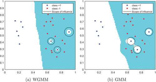
The comparative diagrams for the new influence function we developed and the influence function used in GMM are presented below:

Figure 1 illustrates the influence range of the influence function for both WGMM and GMM. The black circle with the sample as the center is a schematic diagram of the influence range of the sample. Figure 1a provides a schematic depiction of the novel influence function within WGMM. This reveals that diverse samples exhibit varying influence ranges, each with distinct sizes. Figure 1b represents GMM, where the influence ranges for various samples are uniformly sized. During practical model classification, the influence ranges between samples may overlap and converge.

Figure 1. An illustrative example employing synthetic data is used to demonstrate the value range of the memory influence function in linear WGMM and linear GMM. The schematic illustrates classification performance of WGMM when (a) is ${\lambda }_1=4$, ${\lambda }_2=2.30$, ${\lambda }_3=11.31$ and ${\lambda }_4=4$ utilizing the influence range defined in Equation (22)(22) $\mathit{\delta }({\mathbf{x}}_i,{\mathbf{x}}_j)=\exp \left(-\frac{18\parallel {\mathbf{x}}_i-{\mathbf{x}}_j{\parallel }^2}{d^2}\right).$(22) as the memory influence function. (b) is a schematic diagram of the classification performance of GMM when $\mathit{\lambda }=11.31$ and $\mathit{\mu }=111.43$ and the influence range of the RBF kernel as a memory influence function.

Finally, we summarize the procedure of our WGMM with the new memory influence function in Algorithm 1.

Table

Algorithm 1 WGMM with memory influence function (22)
Input: Training set $\mathbf{X}$, and label $\mathbf{Y}$, parameters ${\lambda }_1>0$, ${\lambda }_2>0$, ${\lambda }_3>0$ and ${\lambda }_4>0$, and a kernel function $\mathit{K}(\cdot ,\cdot )$.
1. Divide $\mathbf{X}$ into positive class ${\mathbf{X}}_1$ and negative class ${\mathbf{X}}_2$, where ${\mathbf{X}}_1$ has $\mathit{p}$ samples, and ${\mathbf{X}}_2$ has $\mathit{q}$ samples;
2. for $\mathit{i}=1:\mathit{m}$
${\mathbf{d}}_i=\underset{y_j\ne y_i}{min}||{\mathbf{x}}_i,{\mathbf{x}}_j||;$
end
3. Regarding $d_i$ as $\mathit{d}$ in (22) to calculate ${\mathbf{\Delta }}_{11}$, ${\mathbf{\Delta }}_{12}$, ${\mathbf{\Delta }}_{21}$ and ${\mathbf{\Delta }}_{22}$;
4. Solve problem (17) to obtain $\mathit{\alpha }$ and $\mathit{\beta }$;
5. Substitute $\mathit{\alpha }$ and $\mathit{\beta }$ into (12–14) to obtain $\mathbf{w}$, ${\mathbf{c}}_1$, ${\mathbf{c}}_2$;
6. Substitute $\mathbf{w}$, ${\mathbf{c}}_1$ and ${\mathbf{c}}_2$ into (18–20) to obtain $\mathit{b}$;
Output: $\mathbf{w}$, ${\mathbf{c}}_1$, ${\mathbf{c}}_2$ and $\mathit{b}$.

Experiments

In this section, we describe our experimental study. Section 4.1 lists the datasets and methods used for the experiments. Section 4.2 provides the metrics used to evaluate the performance of all methods, while Sections 4.3 and 4.4 respectively present the specific experiment details and the analysis and summary of the experimental results.

Datasets

Based on 31 datasets obtained from (Rosales-Pérez, Garca, and Herrera 2022), our model is evaluated. Table 1 presents datasets information, including data dimension (n), data volume (m), the size of the positive samples (p), the size of the negative class samples (q), and imbalance ratio (IR) (Lu, Cheung, and Tang 2019) represents the ratio of positive samples to negative samples and is arranged in ascending order of IR values, ranging from small to large. Observing the performance of WGMM in different imbalanced growth scenarios is essential.

Table 1. Description of 31 datasets.

Dataset	m	n	p	q	IR
glass1	214	9	76	138	1.82
ecoli-0 vs 1	220	7	77	143	1.86
wisconsin	683	9	239	444	1.86
pima	768	8	268	500	1.87
glass0	214	9	70	144	2.06
vehicle2	846	18	218	638	2.88
ecoli1	336	7	77	259	3.36
ecoli2	336	7	52	284	5.46
glass6	214	9	29	185	6.38
yeast3	1484	8	163	1321	8.10
ecoli3	336	7	35	301	8.60
yeast-0-3-5-9 vs 7–8	506	8	50	456	9.12
ecoli-0-3-4-7 vs 5–6	257	7	25	232	9.28
ecoli-0-1-4-7 vs 2-3-5-6	336	7	29	307	10.59
yeast-1 vs 7	459	7	30	429	14.30
abalone9–18	731	8	42	689	16.41
glass-0-1-6 vs 5	184	9	9	175	19.44
yeast-1-4-5-8_vs_7	693	8	30	663	22.10
glass5	214	9	9	205	22.78
yeast-2_vs_8	482	8	20	462	23.10
car-good	1728	6	69	1659	24.04
yeast4	1484	8	51	1433	28.10
winequality-red-4	1599	11	53	1546	29.17
poker-9_vs_7	244	10	8	236	29.50
abalone-17 vs 7-8-9-10	2338	8	58	2280	39.31
abalone-21_vs_8	581	8	14	567	40.50
yeast6	1484	8	35	1449	41.40
winequality-white-3–9 vs 5	1482	11	25	1457	58.28
poker-8–9 vs 6	1485	10	25	1460	58.40
poker-8–9 vs 5	2075	10	25	2050	82.00
poker-8 vs 6	1477	10	17	1460	85.88

Performance Metrics

We employed the Geometric Mean (GM) evaluation index from reference (Luque et al. 2019) as the primary evaluation metric in this paper. The evaluation of our model is based on the confusion matrix, as defined in reference (Caelen 2017), which helps in computing key parameters: True Positives (TP), True Negatives (TN), False Positives (FP), and False Negatives (FN). Specifically, TP represents the count of correctly classified positive samples, FP represents the count of misclassified positive samples, TN represents the count of correctly classified negative samples, and FN represents the count of misclassified negative samples. According to the insights presented in reference (Luque et al. 2019), sensitivity and specificity are

(23) $\begin{array}{c}\mathrm{sen}=\frac{\mathrm{TP}}{\mathrm{TP}+\mathrm{FN}},\end{array}$(23)

(24) $\begin{array}{c}\mathrm{spe}=\frac{\mathrm{TN}}{\mathrm{TN}+\mathrm{FP}}.\end{array}$(24)

Then the GM is

(25) $\begin{array}{c}\mathrm{GM}=\sqrt{\mathrm{sen}\ast \mathrm{spe}}.\end{array}$(25)

Reference Methods

The dataset was divided using 10-fold cross-validation. In 10-fold cross-validation, the dataset is randomly separated into 10 distinct subsets. For each fold, one subset is employed as the test set, while the others serve as the training set. Next, 10-fold cross-validation is utilized to select the optimal parameters from within the specified parameter range. Subsequently, these optimal parameters are employed in 20 rounds of 10-fold cross-validation. The number of folds used in each iteration varies, resulting in a total of 200 tests for each dataset.

The comparison methods selected in this paper are LR (LaValley 2008), FSVM-CIL (Batuwita and Palade 2010), GMM (Wang and Shao 2022), SMOTE-SVM (Chawla et al. 2002) and RUS-SVM (He and Garcia 2009). These methods represent advancements in recent years. Linear experiments involving these methods were conducted on 31 datasets, while 17 datasets were chosen for nonlinear experiments. The experiment presents certain challenges related to hyperparameter selection. For the regularization coefficient, we selected a parameter range represented as $\{2^i|\mathit{i}=-8,-6,\dots ,6\}$. In the case of the kernel function parameters in the nonlinear experiments, the range is $\{2^i|\mathit{i}=-10,-8,\dots ,10\}$. All these models were implemented on a personal computer equipped with an Intel Core dual-core processor (dual 4.2 GHz) and 32GB of RAM using MATLAB 2017a. The Quadratic Programming Problems for these models were solved using the same algorithm and tolerance.

Experiments Results and Discussion

In this section, we offer a comparative analysis of the performance of WGMM and alternative methods. We conduct experiments using 31 datasets for linear analysis and 17 datasets for nonlinear studies. Table 2 presents the results of the linearity experiments conducted by each approach. Table 3 presents a selection of datasets that illustrate the non-linear experimental findings for each method. And Figure 2 illustrates the overall effects of each approach on all datasets. Meanwhile, Figure 3 displays the optimal parameters ${\lambda }_1$ and ${\lambda }_2$ selected by the WGMM method during the experiments. And Figure 4 portrays the model results with different parameters using example data. Additionally, Figure 5 highlights the relationship between data parameters and indicators.

Figure 2. (a) depicts the GM distribution for 31 datasets across 5 linear algorithms. (b) illustrates the GM distribution for 17 datasets using 5 nonlinear algorithms.

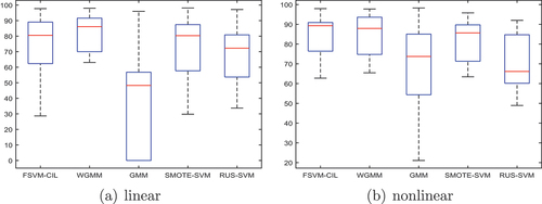
Figure 3. (4) the optimal reference ratio between ${\lambda }_1$ and ${\lambda }_2$ in the formula. (a) is the linear WGMM algorithm. (b) is the nonlinear WGMM algorithm.

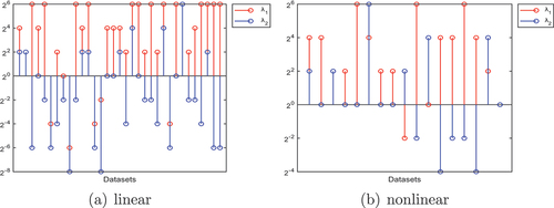
Figure 4. Results of dataset yeast-1-4-5-8, where the $1\mathit{st}$ and $4\mathit{th}$ dimensions are selected.

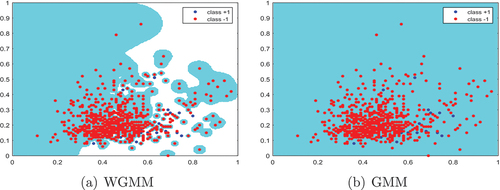
Figure 5. On the datasets of different IR, the GM value of the WGMM method in the selected parameter range. (a)glass0, (b)vehicle2, (c)ecoli1, (d)ecoli3, (e)abalone9–18,(f)winequality-red-4, (g)yeast6,(h)poker-8–9 vs 6, (i)poker-8 vs 6.

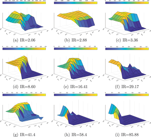
Table 2. GM comparison of linear experiments.

Dataset	IR	LR	FSVM-CIL	WGMM	GMM	SMOTE-SVM	RUS-SVM
glass1	1.82	53.27$\pm$1.82	66.05$\pm$0.81	66.54$\pm$1.46	77.42$\pm$2.04	43.36$\pm$3.70	49.78$\pm$0.00
ecoli-0 vs 1	1.86	97.13$\pm$0.35	97.40$\pm$0.47	97.97$\pm$0.66	95.96$\pm$0.84	97.66$\pm$0.31	94.03$\pm$0.00
wisconsin	1.86	96.35$\pm$0.21	97.72$\pm$0.25	97.70$\pm$0.15	90.01$\pm$0.43	76.73$\pm$0.58	97.14$\pm$0.00
pima	1.87	71.22$\pm$0.48	73.44$\pm$0.43	75.16$\pm$0.66	68.43$\pm$0.48	56.14$\pm$0.64	62.62$\pm$0.00
glass0	2.06	71.41$\pm$0.93	73.98$\pm$1.00	73.18$\pm$1.70	69.47$\pm$1.83	70.38$\pm$0.81	71.02$\pm$0.00
vehicle2	2.88	95.73$\pm$0.31	96.26$\pm$0.36	97.23$\pm$0.22	53.19$\pm$0.75	95.00$\pm$0.43	93.70$\pm$0.00
ecoli1	3.36	84.21$\pm$0.81	89.19$\pm$0.64	89.36$\pm$1.05	73.31$\pm$3.31	87.70$\pm$0.90	87.63$\pm$0.00
ecoli2	5.46	77.60$\pm$0.83	88.64$\pm$0.91	91.58$\pm$0.54	52.34$\pm$2.07	85.70$\pm$0.45	79.83$\pm$0.00
glass6	6.38	89.12$\pm$1.46	90.32$\pm$1.68	92.44$\pm$0.89	57.72$\pm$7.04	87.73$\pm$1.43	80.04$\pm$0.00
yeast3	8.10	81.82$\pm$0.60	88.33$\pm$0.35	91.48$\pm$0.38	50.59$\pm$7.54	89.74$\pm$0.20	85.50$\pm$0.00
ecoli3	8.60	68.80$\pm$2.08	86.71$\pm$0.84	89.43$\pm$1.31	52.23$\pm$6.53	86.60$\pm$0.79	83.85$\pm$0.00
yeast-0-3-5-9 vs 7–8	9.12	54.36$\pm$0.70	64.19$\pm$2.05	68.61$\pm$2.35	53.97$\pm$4.24	62.71$\pm$1.19	57.31$\pm$0.00
ecoli-0-3-4-7 vs 5–6	9.28	87.76$\pm$1.35	90.47$\pm$1.10	91.42$\pm$1.18	0.00$\pm$0.00	85.41$\pm$0.79	81.12$\pm$0.00
ecoli-0-1-4-7 vs 2-3-5-6	10.59	83.70$\pm$1.64	84.77$\pm$3.04	86.10$\pm$1.56	0.00$\pm$0.00	84.72$\pm$0.87	78.13$\pm$0.00
yeast-1 vs 7	14.30	38.30$\pm$2.19	58.23$\pm$3.72	75.64$\pm$1.18	45.94$\pm$4.72	73.05$\pm$0.73	66.27$\pm$0.00
abalone9–18	16.41	68.60$\pm$1.58	80.51$\pm$1.08	84.12$\pm$0.65	49.40$\pm$4.27	80.32$\pm$1.18	66.74$\pm$0.00
glass-0-1-6 vs 5	19.44	89.00$\pm$2.79	96.01$\pm$2.63	97.83$\pm$2.04	0.00$\pm$0.00	98.11$\pm$0.49	76.23$\pm$0.00
yeast-1-4-5-8_vs_7	22.10	0.00$\pm$0.00	39.37$\pm$3.04	68.83$\pm$2.08	0.00$\pm$0.00	58.47$\pm$1.34	49.12$\pm$0.00
glass5	22.78	88.38$\pm$2.48	94.07$\pm$4.56	95.08$\pm$2.58	0.00$\pm$0.00	97.94$\pm$0.35	73.54$\pm$0.00
yeast-2_vs_8	23.10	71.50$\pm$1.53	74.08$\pm$0.01	79.93$\pm$2.59	73.37$\pm$1.51	45.72$\pm$2.42	42.53$\pm$0.00
car-good	24.04	48.17$\pm$1.04	85.64$\pm$1.36	95.30$\pm$0.37	49.04$\pm$2.99	93.27$\pm$0.16	91.81$\pm$0.00
yeast4	28.10	38.73$\pm$1.64	79.65$\pm$1.07	84.43$\pm$0.98	0.00$\pm$0.00	74.96$\pm$0.37	72.24$\pm$0.00
winequality-red-4	29.17	44.80$\pm$6.71	59.59$\pm$1.87	69.89$\pm$1.16	47.58$\pm$2.95	58.89$\pm$0.55	53.60$\pm$0.00
poker-9_vs_7	29.50	40.40$\pm$7.15	59.63$\pm$0.16	70.34$\pm$1.67	44.96$\pm$10.54	57.45$\pm$0.86	54.01$\pm$0.00
abalone-17 vs 7-8-9-10	39.31	52.52$\pm$1.91	80.51$\pm$1.08	88.36$\pm$0.58	48.28$\pm$3.34	84.43$\pm$0.40	78.46$\pm$0.22
abalone-21_vs_8	40.50	85.76$\pm$2.05	83.69$\pm$0.96	91.08$\pm$1.84	45.96$\pm$8.77	84.29$\pm$1.01	65.64$\pm$0.00
yeast6	41.40	58.19$\pm$0.77	87.83$\pm$0.90	88.61$\pm$0.83	21.51$\pm$7.36	82.62$\pm$0.73	73.72$\pm$0.00
winequality-white-3–9 vs 5	58.28	18.80$\pm$1.58	61.72$\pm$3.26	68.21$\pm$2.35	0.00$\pm$0.00	53.72$\pm$1.48	49.29$\pm$0.00
poker-8–9 vs 6	58.40	0.00$\pm$0.00	28.68$\pm$9.23	64.92$\pm$1.01	0.00$\pm$0.00	32.93$\pm$2.25	51.27$\pm$0.00
poker-8–9 vs 5	82.00	0.00$\pm$0.00	42.19$\pm$5.92	66.99$\pm$1.06	4.33$\pm$10.63	29.78$\pm$0.80	33.72$\pm$0.00
poker-8 vs 6	85.88	0.00$\pm$0.00	30.47$\pm$9.58	63.07$\pm$1.33	0.00$\pm$0.00	31.49$\pm$1.49	53.38$\pm$1.43

Table 3. GM comparison of nonlinear experiments.

Dataset	IR	FSVM-CIL	WGMM	GMM	SMOTE-SVM	RUS-SVM
glass1	1.82	77.45$\pm$1.17	75.45$\pm$3.44	76.64$\pm$1.34	72.97$\pm$1.73	65.34$\pm$0.00
ecoli-0 vs 1	1.86	97.46$\pm$0.49	97.34$\pm$0.66	98.26$\pm$0.45	66.67$\pm$3.89	50.62$\pm$0.00
wisconsin	1.86	97.95$\pm$0.11	97.76$\pm$0.25	97.87$\pm$0.13	78.08$\pm$0.33	69.56$\pm$0.00
pima	1.87	73.32$\pm$1.10	66.27$\pm$4.43	67.26$\pm$1.00	63.80$\pm$1.36	57.35$\pm$0.00
glass0	2.06	77.56$\pm$1.04	79.51$\pm$1.56	77.23$\pm$1.63	79.99$\pm$1.10	79.43$\pm$0.00
vehicle2	2.88	96.34$\pm$0.28	96.24$\pm$0.46	91.56$\pm$0.76	95.80$\pm$0.50	77.99$\pm$0.00
ecoli1	3.36	89.96$\pm$0.53	87.89$\pm$2.50	88.19$\pm$1.18	88.22$\pm$0.78	88.29$\pm$0.00
ecoli2	5.46	93.13$\pm$0.84	93.51$\pm$0.63	83.98$\pm$1.01	92.60$\pm$0.69	92.01$\pm$0.00
ecoli3	8.60	90.18$\pm$0.17	86.21$\pm$2.33	70.19$\pm$5.75	89.71$\pm$0.89	89.31$\pm$0.00
yeast-0-3-5-9 vs 7–8	9.12	72.57$\pm$1.39	70.37$\pm$2.13	49.95$\pm$3.64	71.69$\pm$1.46	66.16$\pm$0.00
ecoli-0-3-4-7 vs 5–6	9.28	89.37$\pm$1.72	88.84$\pm$3.23	76.45$\pm$3.39	89.83$\pm$1.58	61.09$\pm$0.00
ecoli-0-1-4-7 vs 2-3-5-6	10.59	89.63$\pm$1.05	89.29$\pm$1.17	70.91$\pm$4.83	87.20$\pm$1.50	57.28$\pm$0.00
yeast-1 vs 7	14.30	73.32$\pm$2.90	72.71$\pm$3.69	55.85$\pm$6.95	70.20$\pm$3.52	61.20$\pm$0.00
glass-0-1-6 vs 5	19.44	89.31$\pm$3.52	90.83$\pm$3.23	47.09$\pm$4.55	89.43$\pm$0.78	86.49$\pm$0.00
yeast-1-4-5-8_vs_7	22.10	62.76$\pm$2.90	65.47$\pm$3.36	49.93$\pm$2.08	63.45$\pm$2.11	48.94$\pm$0.00
glass5	22.78	85.26$\pm$4.25	93.84$\pm$3.22	21.08$\pm$22.37	89.91$\pm$1.66	84.12$\pm$0.00
abalone-21_vs_8	40.50	83.29$\pm$2.98	87.93$\pm$3.06	73.74$\pm$5.05	85.67$\pm$1.70	65.05$\pm$0.00

Table 2 displays the evaluation results for linear models using the GM index. It is evident that WGMM exhibits the best overall performance, particularly when the Imbalance Ratio (IR) is large. Moreover, our method is generally better than LR. In addition, GMM has a GM value of 0.00 on 9 datasets. It can be found that the test accuracy of the minority class on these datasets is 0.00. GMM performs poorly on imbalanced data. In terms of variance, WGMM falls within an acceptable range, and RUS-SVM excels, with variance at 0.00 on most datasets.

Table 3 presents the evaluation of nonlinear experiments using the GM index. Notably, the FSVM-CIL model performs well on datasets with a small Imbalance Ratio (IR), and WGMM and FSVM-CIL show comparable performance. However, as the IR increases, WGMM emerges as the leading performer, exhibiting significantly superior results compared to other methods.

Comparing Tables 2 and 3, we find:

1. In Table 3, out of the 17 datasets, 11 of them exhibit a distinctive pattern. Under the GM metric, our linear algorithm outperforms the nonlinear model, which can be attributed to the influence of data characteristics.

2. The datasets ecoli-0-3-4-7 vs 5-6, ecoli-0-1-4-7 vs 2-3-5-6, glass-0-1-6 vs 5, yeast-1-4- 5-8 vs 7 and glass5 exhibited a GM value of 0.00 in the GMM linear experiments. While substantial improvements were observed in the nonlinear experiments, the results remained less than satisfactory.

Figure 2 consists of two boxplots. Figure 2a represents a comparative boxplot of GM values for five methods in the linear experiment. Notably, WGMM exhibits higher median, first quartile, and third quartile values compared to the other methods, with shorter whiskers. This indicates the superior performance of WGMM. Conversely, the GMM method shows a lower box, longer whiskers, and lower outliers, clearly highlighting the subpar performance of unweighted methods in imbalanced experiments. Figure 2b represents the boxplot comparison of the five methods in the nonlinear experiment. Overall, both FSVM-CIL and WGMM methods perform better. Their boxes are short and skewed upward, signifying larger GM values. While the median and first quartile of FSVM-CIL are slightly greater than WGMM, the third quartile of WGMM is larger, and its upper whisker is longer. This suggests that predictive results of WGMM are notably larger.

In formula (4), ${\lambda }_1$ and ${\lambda }_2$ represent the coefficients of the positive and negative class memory cost functions, respectively, with ${\lambda }_1$ referring to the positive class. Owing to the imbalance in sample sizes between the positive and negative classes, applying the same weight would introduce bias into performance of the model, favoring the class with more samples. Hence, it becomes essential to define different weights. The weight for the minority class is increased to balance the model’s performance on both types of samples. Figure 3a is the optimal reference comparison diagram for ${\lambda }_1$ and ${\lambda }_2$ for each dataset in the context of the linear experiment. Figure 3b is the optimal reference comparison diagram for each dataset comparing ${\lambda }_1$ and ${\lambda }_2$ in the context of nonlinear experiments. Most of the datasets show that ${\lambda }_1>{\lambda }_2$. This implies that greater weight is assigned to the minority samples, thereby achieving data balance through varying weights. In situations of class imbalance, the model attains optimal classification.

Figure 4 selects the 1st and 4th dimensions of the dataset yeast-1-4-5-8 vs 7 for training and testing. Figure 4a represents the optimal parameters, specifically ${\lambda }_1=2^2$, ${\lambda }_2=2^{-4}$, ${\lambda }_3=2^0$ and ${\lambda }_4=2^2$. Figure 4b shows the result when the weights of the cost memory function are equal, that is, ${\lambda }_1={\lambda }_2=2^4$. It is evident that Figure 4b, the trained classifier exhibits a bias toward the majority class samples, favoring the negative class. This underscores the importance of weighting.

Figure 5 is the linear experimental GM change plot of different datasets for different ${\lambda }_1$ and ${\lambda }_2$. We can see the following points.

1. Different datasets correspond to different optimal parameters ${\lambda }_1$ and ${\lambda }_2$, which may be affected by the data structure and IR value.

2. In many data sets, when ${\lambda }_1>{\lambda }_2$, the GM value is larger. And the GM value of the model with non-optimal parameters will be partially 0.00.

3. The larger the IR, the fewer parameter groups have a GM value greater than 0.5, and the more parameter groups have a GM value of 0.00.

From the above results, it can be seen that WGMM is a competitive choice.

Conclusions

In this study, our WGMM sets weight parameters for the memory cost functions of positive and negative class samples, respectively. A new adaptive memory influence function is proposed. Implementation samples are described individually without increasing the weight of the entire category. It will not be affected by different training samples and can adapt to different imbalance scenarios. Ensure zero empirical risk while retaining generalization capabilities.

We conduct a comprehensive evaluation of WGMM on 31 imbalanced datasets, benchmarking its performance against alternative methods. Experimental results demonstrate the efficacy of WGMM in tackling imbalanced classification problems and showcasing robust generalization abilities. Notably, in scenarios with a substantial IR, our model exhibits pronounced characteristics and excels across various evaluation metrics.

Regarding the different parameters set for the positive and negative class memory impact functions, experiments found that the optimal parameters of the minority class sample memory impact function are greater than or equal to the optimal parameters of the majority class sample memory impact function. The adaptive memory influence function enables the model to adapt well to different data, and the effect is better than other methods.

These findings strongly affirm WGMM as an effective approach for addressing imbalanced classification challenges. Its superiority in performance and adaptability across different imbalanced datasets without the need for parameter tuning positions WGMM as a potent tool for practical applications.

Future research avenues may involve further optimizing performance of WGMM and exploring its applicability in diverse fields and tasks. In summary, this study provides novel insights and effective solutions for resolving imbalanced classification problems.

Acknowledgements

The authors would like to thank the anonymous reviewers for their valuable suggestions.

Disclosure Statement

No potential conflict of interest was reported by the author(s).

Data Availability Statement

The data that support the findings of this study are available in [IEEE] at [doi: 10.1109/TCYB.2022.3163974], reference (Rosales-Perez, Garca, and Herrera 2022). These data were derived from the following resources available in the public domain: [https://ieeexplore.ieee.org/document/9756639].

Supplementary Material

Supplemental data for this article can be accessed online at https://doi.org/10.1080/08839514.2024.2355424

Additional information

Funding

The work was supported by the National Natural Science Foundation of China [61966024, 62366035]; National Natural Science Foundation of China [62106112]; Natural Science Foundation of Inner Mongolia Autonomous Region [2023MS01006].

References

- Abdelhamid, D., S. Khaoula, and O. Atika. 2014. Automatic bank fraud detection using support vector machines. In The International Conference on Computing Technology and Information Management, Dubai, UAE, January.
- Alfian, G., M. Syafrudin, I. Fahrurrozi, N. L. Fitriyani, F. T. D. Atmaji, T. Widodo, N. Bahiyah, F. Benes, and J. Rhee. 2022. Predicting breast cancer from risk factors using SVM and extra-trees-based feature selection method. Computers 11 (9):136. doi:10.3390/computers11090136.
- Bach, F. R., D. Heckerman, and E. Horvitz. 2006. Considering cost asymmetry in learning classifiers. Journal of Machine Learning Research 7:1713–20.
- Batuwita, R., and V. Palade. 2010. FSVM-CIL: Fuzzy support vector machines for class imbalance learning. IEEE Transactions on Fuzzy Systems 18 (3):558–71. doi:10.1109/TFUZZ.2010.2042721.
- Caelen, O. 2017. A Bayesian interpretation of the confusion matrix. Annals of Mathematics and Artificial Intelligence 81 (3–4):429–50. doi:10.1007/s10472-017-9564-8.
- Chaabane, S. B., M. Hijji, R. Harrabi, and H. Seddik. 2022. Face recognition based on statistical features and SVM classifier. Multimedia Tools & Applications 81 (6):8767–84. doi:10.1007/s11042-021-11816-w.
- Chawla, N. V., K. W. Bowyer, L. O. Hall, and W. P. Kegelmeyer. 2002. SMOTE: Synthetic minority over-sampling technique. The Journal of Artificial Intelligence Research 16:321–57. doi:10.1613/jair.953.
- Chen, C., X. Xu, G. Wang, and L. Yang. 2022. Network intrusion detection model based on neural network feature extraction and PSO-SVM. In 2022 7th International Conference on Intelligent Computing and Signal Processing (ICSP), Xi’an, China, April, 1462–65.
- Datta, S., and S. Das. 2015. Near-Bayesian support vector machines for imbalanced data classification with equal or unequal misclassification costs. Neural Networks 70:39–52. doi:10.1016/j.neunet.2015.06.005.
- Fletcher, R. 2000. Practical methods of optimization. New Jersey, USA: JohnWiley & Sons.
- Hamdan, Y. B., and A. Sathesh. 2021. Construction of statistical SVM based recognition model for handwritten character recognition. Journal of Information Technology and Digital World 3 (2):92–107. doi:10.36548/jitdw.2021.2.003.
- Hart, P. 1968. The condensed nearest neighbor rule (corresp.). IEEE Transactions on Information Theory 14 (3):515–16. doi:10.1109/TIT.1968.1054155.
- Harvianto, H., L. Ashianti, J. Jupiter, and S. Junaedi. 2016. Analysis and voice recognition in Indonesian language using MFCC and SVM method. ComTech: Computer, Mathematics and Engineering Applications 7 (2):131–39. doi:10.21512/comtech.v7i2.2252.
- He, H., Y. Bai, E. A. Garcia, and S. Li. 2008. ADASYN: Adaptive synthetic sampling approach for imbalanced learning. In 2008 IEEE International Joint Conference on Neural Networks, Hong Kong, China, June, 1322–28.
- He, H., and E. A. Garcia. 2009. Learning from imbalanced data. IEEE Transactions on Knowledge and Data Engineering 21 (9):1263–84. doi:10.1109/TKDE.2008.239.
- Hussain, M., S. K. Wajid, A. Elzaart, and M. Berbar. 2011. A comparison of SVM kernel functions for breast cancer detection. In 2011 Eighth International Conference Computer Graphics, Imaging and Visualization, Singapore, August, 145–50.
- Imam, T., K. M. Ting, and J. Kamruzzaman. 2006. z-SVM: An SVM for improved classification of imbalanced data. In AI 2006: Advances in Artificial Intelligence: 19th Australian Joint Conference on Artificial Intelligence, Proceedings, Hobart, Australia, Vol. 19, 264–73.
- Iranmehr, A., H. Masnadi-Shirazi, and N. Vasconcelos. 2019. Cost-sensitive support vector machines. Neurocomputing 343:50–64. doi:10.1016/j.neucom.2018.11.099.
- Kibria, M. R., A. Ahmed, Z. Firdawsi, and M. A. Yousuf. 2020. Bangla compound character recognition using support vector machine (SVM) on advanced feature sets. In 2020 IEEE Region 10 Symposium, Dhaka, Bangladesh, 965–68.
- Krawczyk, B. and M. Woźniak. 2015. Cost-sensitive neural network with roc-based moving threshold for imbalanced classification. In 16th International Conference, Wroclaw, Poland, October 14–16, 2015, Proceedings 16, 45-52.
- Krawczyk, B., M. Woźniak, and G. Schaefer. 2014. Cost-sensitive decision tree ensembles for effective imbalanced classification. Applied Soft Computing 14:554–62. doi:10.1016/j.asoc.2013.08.014.
- Kumar, M., R. K. Sharma, and M. K. Jindal. 2011. SVM based offline handwritten Gurmukhi character recognition. SCAKD Proceedings 758:51–62.
- LaValley, M. P. 2008. Logistic regression. Circulation 117 (18):2395–99. doi:10.1161/CIRCULATIONAHA.106.682658.
- Lilhore, U. K., S. Simaiya, H. Pandey, V. Gautam, A. Garg, and P. Ghosh. 2022. Breast Cancer Detection in the IoT Cloud-based Healthcare Environment Using Fuzzy Cluster Segmentation and SVM Classifier. In Ambient Communications and Computer Systems. Lecture Notes in Networks and Systems, ed. Y. Hu, S. Tiwari, M. C. Trivedi, and K. K. Mishra. Vol. 356. Singapore: Springer.
- Lu, Y., Y. M. Cheung, and Y. Y. Tang. 2019. Bayes imbalance impact index: A measure of class imbalanced data set for classification problem. IEEE Transactions on Neural Networks and Learning Systems 31 (9):3525–39. doi:10.1109/TNNLS.2019.2944962.
- Luo, H., X. Pan, Q. Wang, S. Ye, and Y. Qian 2019. Logistic regression and random forest for effective imb alanced classification. In 2019 IEEE 43rd Annual Computer Software and Applications Conference (COMPSAC), Milwaukee, WI, USA. 1:916–17.
- Luque, A., A. Carrasco, A. Martin, and A. de Las Heras. 2019. The impact of class imbalance in classification performance metrics based on the binary confusion matrix. Pattern Recognition 91:216–31. doi:10.1016/j.patcog.2019.02.023.
- Mathew, J., C. K. Pang, M. Luo, and W. H. Leong. 2017. Classification of imbalanced data by oversampling in kernel space of support vector machines. IEEE Transactions on Neural Networks and Learning Systems 29 (9):4065–76. doi:10.1109/TNNLS.2017.2751612.
- Nasien, D., H. Haron, and S. S. Yuhaniz. 2010. Support Vector Machine (SVM) for English handwritten character recognition. In 2010 2nd International Conference on Computer Engineering and Applications, Bali Island, 1:249–52.
- Nguyen, H. M., E. W. Cooper, and K. Kamei. 2011. Borderline over-sampling for imbalanced data classification. International Journal of Knowledge Engineering and Soft Data Paradigms 3 (1):4–21. doi:10.1504/IJKESDP.2011.039875.
- Rosales-Pérez, A., S. Garca, and F. Herrera. 2022. Handling imbalanced classification problems with support vector machines via evolutionary bilevel optimization. IEEE Transactions on Cybernetics 53 (8):4735–47. doi:10.1109/TCYB.2022.3163974.
- Seo, H., L. Brand, L. S. Barco, and H. Wang. 2022. Scaling multi-instance support vector machine to breast cancer detection on the BreaKHis dataset. Bioinformatics 38 (Supplement_1):92–100. doi:10.1093/bioinformatics/btac267.
- Sudha, C., and D. Akila. 2021. Credit card fraud detection system based on operational & transaction features using svm and random forest classifiers. In 2021 2nd International Conference on Computation, Automation and Knowledge Management (ICCAKM), Dubai, United Arab Emirates, 133–38.
- Sui, Y., Y. Wei, and D. Zhao. 2015. Computer-aided lung nodule recognition by SVM classifier based on combination of random undersampling and SMOTE. Computational & Mathematical Methods in Medicine 2015:1–13. doi:10.1155/2015/368674.
- Vapnik, V., and R. Izmailov. 2021. Reinforced SVM method and memorization mechanisms. Pattern Recognition 119:108018. doi:10.1016/j.patcog.2021.108018.
- Wang, Z., and Y. H. Shao. 2022. Generalization-Memorization Machines. arXiv preprint arXiv:2207.03976.
- Xiong, Y., and R. Zuo. 2020. Recognizing multivariate geochemical anomalies for mineral exploration by combining deep learning and one-class support vector machine. Computers & Geosciences 140:104484. doi:10.1016/j.cageo.2020.104484.
- Zhang, S., Q. Fu, and W. Xiao. 2017. Advertisement click-through rate prediction based on the weighted-ELM and adaboost algorithm. Scientific Programming 2017:2938369. doi:10.1155/2017/2938369.
- Zheng, X. 2020. SMOTE variants for imbalanced binary classification: Heart disease prediction. Ann Arbor, Michigan, USA: Los Angeles ProQuest Dissertations Publishing. University of California.