Entropy-based deep neural network training optimization for optical coherence tomography imaging

ABSTRACT

This paper presents an optimization technique for the number of training epochs needed for deep learning models. The proposed method eliminates the need for separate validation data and significantly decreases training epochs. Using a four-class Optical Coherence Tomography (OCT) image dataset encompassing Choroidal Neovascularization (CNV), Diabetic Macular Edema (DME), Drusen, and Normal retina categories, we evaluated twelve architectures. These include general-purpose models (Alexnet, VGG11, VGG13, VGG16, VGG19, ResNet-18, ResNet-34, and ResNet-50) and OCT image-specific models (RetiNet, AOCT-NET, DeepOCT, and Octnet). The proposed technique reduced training epochs ranging from 4.35% to 58.27% for all architectures except Alexnet. Although the overall increase in accuracy ranges from 0.28% to 12.6%, with some architectures experiencing minor improvements, this is seen as acceptable considering the substantial reduction in training time. By achieving higher accuracy with fewer training epochs and eliminating the need for separate validation data, our methodology streamlines early stopping significantly. Statistical evaluations via Shapiro-Wilk and Kruskal-Wallis tests further affirm these results, showcasing the potential of this novel technique for efficient deep learning practices in scenarios constrained by time or computational resources.

Introduction

Optical Coherence Tomography (OCT) is a noninvasive imaging technique that uses interferometry-based technology to produce high-resolution cross-sectional images of the retina (Irsch 2021). OCT is primarily used for diagnosing retinal diseases (Podoleanu 2012). Convolutional neural networks (CNNs) have been extensively researched and have shown remarkable performance in addressing image and speech recognition challenges, including natural language processing (Gu et al. 2018). A typical CNN has pooling layers for downsampling, convolution layers for creating ’feature maps,’ and a fully connected layer after several rounds of convolution and pooling layers (Lindsay 2021).

(1) $(\mathit{F}\ast \mathit{k})(\mathit{p})=\sum _{\mathit{s}+\mathit{t}=\mathit{p}}\mathit{F}(\mathit{s})\mathit{k}(\mathit{t})$(1)

Equation 1(1) $(\mathit{F}\ast \mathit{k})(\mathit{p})=\sum _{\mathit{s}+\mathit{t}=\mathit{p}}\mathit{F}(\mathit{s})\mathit{k}(\mathit{t})$(1) represents convolution, where the convolution kernel is denoted by $\mathit{k}$, and the kernel values are known as weights. Convolution plays a crucial role in feature extraction with its ability to recognize image patterns. The convolution outputs are known as feature maps. Node values in the fully connected layer, also known as weights, signify the relevance of a feature, with the strength of the feature directly proportional to the node value. Parameters such as loss function (Janocha and Czarnecki 2017), learning rate (Brownlee 2020), sample size, and the number of iterations must be pre-defined before training a CNN. AlexNet’s 2012 debut sparked a wave of advancements in CNN architectures (Krizhevsky, Sutskever, and Hinton 2012), with focus on optimizing depth, feature mapping, and training methods (Karthik and Mahadevappa 2023; Lindsay 2021; Narkhede, Bartakke, and Sutaone 2022; Rawat and Wang 2017). Training, requiring initial weight setup, aims to minimize prediction error. Standard performance parameters like Sensitivity, Specificity, Precision, and F1 score are calculated post-training (Powers 2020), limiting real-time control during training. Validation data aids in real-time monitoring but reduces training data, affecting classification accuracy.

Entropy, a concept from information theory, measures the variability in data, reflecting its information content (Shannon 1948). It serves as a unit of measurement for information, choice, and uncertainty (Shannon 1948). Entropy quantifies the number of choices involved and the certainty of the outcome.

(2) $\mathit{E}=-\sum _i{p}_i\log p_i$(2)

$\mathit{E}$ represents Shannon entropy, with probability values $p_i$ obtained from the histogram. Training optimization with early stopping prevents overfitting, a condition in which the model gets biased toward the training data, lowering its generalization ability and accuracy. Early stopping approaches have been studied for over 20 years, and early stopping without a validation dataset is still being researched (Bonet et al. 2021; Forouzesh and Thiran 2021; Li et al. 2021; Mahsereci et al. 2017). Backpropagating supervisory signals in training shows that signals from one layer can govern the complete model’s training (Bai et al. 2021). Early stopping techniques utilizing the entire dataset include using the data directly (Raskutti, Wainwright, and Yu 2014) or using a parallel-trained neural network (Li et al. 2021; Vardasbi, de Rijke, and Dehghani 2022). Training data-based early stopping strategies include signal-to-noise ratio figure (SNRF) estimates, also known as goodness-of-fit approximation and gradient disparity (Forouzesh and Thiran 2021; Liu, Starzyk, and Zhu 2008). The fixed number of nodes in a CNN’s neural network makes it similar to a parametric machine learning model. Early stopping without a validation dataset is done via entropy analysis of the posterior distribution of the parametric vector $\mathit{w}$ (Duvenaud, Maclaurin, and Adams 2016). Information theory-based analysis is used to quantify learning algorithms’ generalization capacity (Bu, Zou, and Veeravalli 2020; Steinke and Zakynthinou 2020; Xu and Raginsky 2017). Information theory-based loss functions give deep classification networks label-noise invariance (Xu et al. 2019). Entropy helps optimize neural networks through network pruning (Liu, Ali Amjad, and Geiger 2018) or quantization for deployment in resource-constrained contexts, such as mobile devices (Park, Ahn, and Yoo 2017). Entropy has been utilized to train neural networks with backpropagation instead of mean squared error (Silva, de Sá, and Alexandre 2005). Entropy is also used to map artificial neural networks to real neurons and as a feature in neural networks for computer-assisted epilepsy diagnosis from EEG (Srinivasan, Eswaran, and Sriraam 2007). Adaptive networks use entropy in the retraining step to increase artificial neural network accuracy (Pinto, Morais, and Corchado 2019).

Although entropy has been extensively employed in deep learning, its use for early stopping during neural network training remains an unexplored area. We propose a system that leverages entropy to regulate the training process, stopping it when specific conditions are satisfied. Our paper examines the impact of entropy on the training process and compares the results with those obtained by monitoring validation loss using a separate validation set. Our study neither uses external data, separate validation data, nor training data; it uses entropy, a statistical value computed from the weight matrix during training, for optimized training of CNNs. An entropy-based early stopping technique eliminates the need for validation data to monitor and control deep neural networks while reducing the number of training epochs needed. This approach aims to provide a more resource-efficient yet effective solution for training deep learning models. Our approach is independent of the type and size of the dataset since the threshold value ($\mathit{\delta }$), which determines the termination condition, is determined dynamically using the initial entropy calculated from the weights. The proposed technique calculates entropy from the first fully connected layer. Since most CNN classification architectures will have at least one fully connected layer, the proposed technique can be used with various CNN architectures. Images directly influence what features the feature maps detect, but the fully connected layer’s weights are less dependent on specific visual features. Therefore, the proposed technique could work with CNNs to classify other types of images.

Method

Overview

Deep neural networks, including those used in healthcare applications, perform optimally when provided with a large amount of training data. When constructing a model, it is common to divide the available data into three sets: training, validation, and testing. Traditionally, having a validation set has been the most commonly used approach to adjust the model and prevent overfitting, as it enables researchers to fine-tune the model’s parameters based on its performance on unseen data. This, in turn, helps in identifying an optimal balance between the model’s ability to fit the training data and its generalization to new, unseen data, thereby reducing the risk of overfitting. Our research aims to propose an alternate network training optimization technique that does not require separate validation data. Our methodology proposes the use of entropy as a measure for early stopping. We have conducted tests on twelve different architectures. These architectures include all variations within VGG (Simonyan and Zisserman 2014), AlexNet (Krizhevsky, Sutskever, and Hinton 2012), and ResNet (He et al. 2016) and architectures designed specifically for OCT image classification, such as AOCT-NET (Alqudah 2020), RetiNet (Apostolopoulos et al. 2017), DeepOCT (Altan 2022), and Octnet (Sunija et al. 2021). In our evaluation, we compared the results obtained using validation data for early stopping with those achieved using the proposed early stopping technique, which does not require validation data. To implement our methodology, we utilized the Python programming language and various libraries, such as TensorFlow, NumPy, Scikit-learn, and Matplotlib.

Data

The data used in the study is available as a public dataset under a CC BY-NC-SA 4.0 license. The dataset contains 84,495 images in four classes: Choroidal Neovascularization (CNV), Diabetic Macular Edema (DME), early AMD Drusen, and Normal retina (Kermany, Zhang, and Goldbaum 2018). The dataset consists of 37,205 images categorized as CNV 11,348 images categorized as DME, 8,616 images categorized as Drusen, and 26,315 images categorized as Normal. In order to simplify implementation, the images have been resized to 100 × 100. The dataset can be accessed via the Mendeley data repository (Kermany, Zhang, and Goldbaum 2018). The authors of the dataset have already segregated the dataset; this eliminates any concern regarding bias while testing the model to generate the results. No pre-processing was used to maintain uniformity across general-purpose and OCT-specific architectures. Given the small original validation set, we partitioned the data with 80% as training data and 20% as validation data while preserving the ratio of images in each class, preventing the introduction of any class bias in the model.

Algorithm Development

CNNs update weights across all layers simultaneously. Hence, we can effectively monitor the entire network’s training by focusing on dense layers. Layer-wise analysis is already being used to analyze the performance of CNNs (Bai et al. 2021). Tracking dense layers provides two primary advantages: reduced dimensionality and condensed information from all feature layers. The optimal dense layer for monitoring is the first because its inputs contain features from convolution layers learned from data. Monitoring neurons in a layer is essentially equivalent to monitoring weight updates. These changes can be observed directly, or the updated weights can be tracked. As networks are trained through optimization, the focus shifts toward the significance of the optimization outcome rather than the process itself. Thus, our study focuses on monitoring and utilizing the optimization outcome to guide network training. The weights are interpreted and analyzed as information. Consequently, our study employs entropy to track the training process and stop the training once the change in entropy drops below a predetermined threshold.

An epoch signifies a complete cycle where the entire dataset is used once in the learning process. Extensive training can enhance the model’s accuracy on the training data, but it’s essential to be wary about overfitting and ensure that the epoch count is adequately controlled. Consequently, significant assessments and decisions are made at epoch terminations. Our calculations are performed at the fully connected layer level, encompassing all neurons rather than focusing on individual ones. The weight vector, with dimensions equal to the number of neurons in the layer, is converted into a tensor to facilitate faster computations. The distribution of the trained weights is influenced by the weight initialization. As the network undergoes training, the deviation of weight values initially rises and gradually decreases as the weight values stabilize (Sinha et al. 2017; Yilmaz and Poli 2022). When non-uniform weight initializations are used, the network training leads to a higher standard deviation in the distribution of weights (Sinha et al. 2017). This causes the distribution to become more spread out, indicating increased uncertainty and entropy. The entropy of the fully connected layer will continue to increase during training and cease to change once the optimal weights have been learned. In the case of sensitive networks, continued training after optimal weights should be observed as a reduction in entropy value. Multiple fully interconnected network layers necessitate that the relationship between multiple events be taken into account. The events within a single layer will be independent, whereas the same events witnessed from the subsequent layer will be dependent. Assume that two adjacent layers, $\mathit{x}$ and $\mathit{y}$, each containing $\mathit{m}$ and $\mathit{n}$ nodes, and that $\mathit{p}(\mathit{i},\mathit{z})$ is the joint probability.

(3) $\mathit{E}(\mathit{x},\mathit{y})=-\sum _{\mathit{iz}}\mathit{p}(\mathit{i},\mathit{z})\log \mathit{p}(\mathit{i},\mathit{z})$(3)

While,

(4) $\mathit{E}(\mathit{x})=-\sum _{\mathit{iz}}\mathit{p}(\mathit{i},\mathit{z})\log \sum _z\mathit{p}(\mathit{i},\mathit{z})$(4)

(5) $\mathit{E}(\mathit{y})=-\sum _{\mathit{iz}}\mathit{p}(\mathit{i},\mathit{z})\log \sum _i\mathit{p}(\mathit{i},\mathit{z})$(5)

(6) $\mathit{E}(\mathit{x},\mathit{y})\le \mathit{E}(\mathit{x})+\mathit{E}(\mathit{y})$(6)

Equality occurs when both events are independent (Shannon 1948).

(7) $\mathit{p}(\mathit{i},\mathit{z})=\mathit{p}(\mathit{i})\mathit{p}(\mathit{z})$(7)

In the absence of independence, conditional entropy $($$E_x(\mathit{y})$$)$ is used, which is defined as:

(8) $E_x(\mathit{y})=-\sum _{\mathit{iz}}\mathit{p}(\mathit{i},\mathit{z})\log p_i(\mathit{z})$(8)

The joint entropy can now be expressed as:

(9) $\mathit{E}(\mathit{x},\mathit{y})=\mathit{E}(\mathit{x})+E_x(\mathit{y})$(9)

As seen in equation 9(9) $\mathit{E}(\mathit{x},\mathit{y})=\mathit{E}(\mathit{x})+E_x(\mathit{y})$(9) , a linear relationship between the total entropy of both layers and their individual entropies enables learning based solely on entropy. Error backpropagation necessitates a linear relationship for simplicity and ease of implementation. A linear relationship ensures the independence of the terms’ derivatives; consequently, the update of the weights within the layer is also independent.

Our method calculates the entropy of the weight matrix in the first fully connected layer. The first fully connected layer is the ideal choice, as it is an essential component in every CNN architecture. Furthermore, as previously stated, selecting the first fully connected layer is the most advantageous when dealing with multiple fully connected layers since it contains the highest amount of information. A custom callback function was designed to be invoked at the termination of each epoch. The commands within this function are presented in Algorithm 1. In this function, which gets executed at epoch termination, the weight matrix is extracted, and its entropy is computed. If the change in entropy value ($\mathrm{\Delta }{e}_{\mathit{ij}}$) meets the threshold value ($\mathit{\delta }$), training is terminated. The conversion of the weight matrix to a list in Algorithm 1 is primarily a programming convenience and does not possess any specific technical significance.

Table

Algorithm 1: Monitoring and termination of training using entropy.
1 Store the weight matrix of fully connected layer after each epoch.
2 Compute entropy of the weight matrix $\mathit{W}$ between two adjacent layers $\mathit{x}$ and $\mathit{y}$.
(10) $e_k=\mathit{E}(W_k;x_i,y_z)$(10)
3 Store the entropy values in the form of a list.
4 Compute $\mathit{\delta }$ using initial rate of change of entropy
(11) $\mathit{\delta }=\frac{e_{01}^{\prime }}{10}$(11)
$e_{01}\prime$ represents the initial change in entropy after the second epoch.
5 Compare the entropy of the current epoch with the previous, and stop the training if the following conditions are met:
(12) $\mathrm{\Delta }{e}_{\mathit{ij}}<\mathit{\delta }\text{amp}\mathit{\alpha }>{\alpha }_0$(12)

The value of $\mathit{\delta }$ must either be predetermined or dynamically determined based on the initial entropy values (Equation 11). In order to enhance the algorithm’s overall generalizability, we opted to dynamically assign the value of $\mathit{\delta }$ (Equation 11). $\mathit{\alpha }$ records the current epoch value, and ${\alpha }_0$ is a pre-set constant that holds the value of the minimum number of epochs the network should run for. The default value of ${\alpha }_0$ is three. During the training loop, the callback function is executed after each epoch. Within this callback function, the entropy, accuracy, and loss parameters are computed. These values are stored in a global object that can be accessed outside of the training loop for plotting accuracy curves and calculating performance metrics such as Sensitivity, Specificity, Precision, and F1 score. The confusion matrix, which indicates class-wise performance, is calculated outside the training loop as well. The entire experiment is repeated thirty times, with the learning rate being incremented by a small amount each time (Equation 13(13) ${\gamma }_k=\mathit{\gamma }(\frac{k}{5}+1);\mathit{k}\in [0,29]$(13) ). This process aims to document changes in evaluation parameters at different learning rates, which is necessary to eliminate any dependency between the algorithm’s performance and the learning rate. The same hyperparameters are used across different architectures to enable a comparison between the architectures themselves. Each network architecture is tested using two separate configurations: one that employs validation data for early stopping and another that utilizes the proposed method without validation data for early stopping. For this study, the following hyperparameter values were employed:

• Learning rate ($\mathit{\gamma }$): 0.001

• Patience value(validation set): 7

• Batch size: 128

• The formula for the learning rate for the $k^{\mathrm{th}}$ iteration of the model:

(13) ${\gamma }_k=\mathit{\gamma }(\frac{k}{5}+1);\mathit{k}\in [0,29]$(13)

Ensuring consistency by using the same hyperparameters across all networks allows for direct comparisons of results. These hyperparameters were empirically chosen to achieve the highest accuracy.

Algorithm Evaluation

The proposed early stopping technique is integrated with various deep learning architectures, including multiple versions of VGG and ResNet, as well as AlexNet, AOCT-NET, RetiNet, DeepOCT, and Octnet. We conducted a thorough evaluation and comparison of the model’s performance; this assessment considered the accuracy and the number of epochs needed for convergence in each case. Our graphical analysis includes the analysis of the training curves in each case, which are selected randomly across the thirty different learning rates. Comparing training curves obtained from three other runs, each with a different learning rate eliminates any learning-rate-specific biases. To enable a comprehensive comparison across all learning rates, we plotted accuracy-epoch values to analyze the distribution and identify patterns. By examining the regression lines, we could discern trends and relationships between learning rates, accuracy, and the number of epochs needed for convergence. For statistical analysis, we first conducted the Shapiro-Wilk test for normality on the number of epochs needed for training each architecture across thirty different learning rates, both with and without validation data. Following this, we performed the Kruskal-Wallis test to determine the statistical significance of differences between groups in order to gain a clearer understanding of the impact of the proposed early stopping technique.

Results

Experimental Setup

Utilizing a publicly accessible OCT dataset (Kermany, Zhang, and Goldbaum 2018), we evaluated our entropy-based early stopping method. The dataset is available for download via the Mendeley data repository (Kermany et al. 2018). The dataset consists of images categorized into four different classes which are Choroidal Neovascularization (CNV), Diabetic Macular Edema (DME), Drusen and normal. The twelve architectures used for comparison in our study include Alexnet (Krizhevsky, Sutskever, and Hinton 2012), all VGG (Simonyan and Zisserman 2014) and ResNet (He et al. 2016) versions, and OCT-specific architectures such as AOCT-NET (Alqudah 2020), RetiNet (Apostolopoulos et al. 2017), DeepOCT (Altan 2022), and Octnet (Sunija et al. 2021). We ensured that the testing methodology was consistent with the techniques used by the authors of architectures under study, which involves using a test set. Since the main focus is not on achieving the highest accuracy but on optimizing the training process itself, it is essential to keep the hyperparameters consistent across all architectures under study. Each architecture under study is run thirty times for the different learning rates, with the learning rate calculated as shown in Equation 13.(13) ${\gamma }_k=\mathit{\gamma }(\frac{k}{5}+1);\mathit{k}\in [0,29]$(13)

Analysis

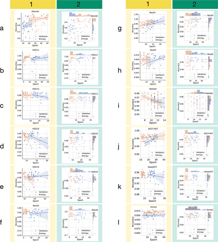
In this study, we graphically represent the analysis in training curves for three unique runs, each employing a different learning rate, randomly selected from a total of thirty. The training curves for the traditional validation data-based method illustrate accuracy curves for both training and validation data, while those for our proposed entropy-based technique display the training data accuracy curve and the entropy curve (E1). This process is executed for each of the twelve architectures under study, comparing both the conventional validation data method for early stopping and our proposed entropy-based method. The resultant data is distributed across six figures (Figures 1–6) to facilitate a more accessible visualization and interpretation of the plots. In Figure 7, we plotted accuracy-epoch values for different learning rates to analyze the distribution and identify patterns. By examining the regression lines, we could discern trends and relationships between accuracy and the number of epochs needed for convergence for different learning rates.

Figure 1. Training curves comparing four architectures using validation data based approach.

Sub-figures (a) Alexnet, (b) VGG11, (c) VGG13, (d) VGG16, illustrating the performance of each architecture when utilizing a validation data based approach for early stopping.

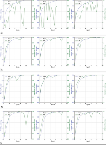
Figure 2. Training curves comparing four architectures using proposed entropy-based method.

Sub-figures (a) AlexNet, (b) VGG11, (c) VGG13, (d) VGG16 demonstrating the performance of each architecture when utilizing the proposed entropy-based method for early stopping.

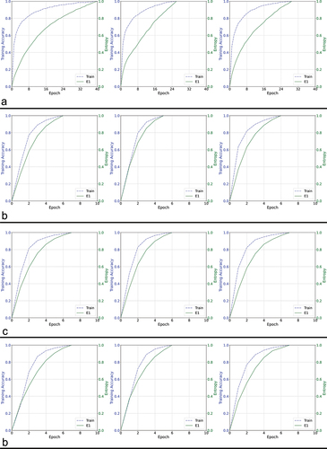
Figure 3. Training curves comparing a different set of four architectures using validation data based approach.

Sub-figures (a) VGG19, (b) ResNet-18, (c) ResNet-34, (d) ResNet-50, illustrating the performance of each architecture when utilizing a validation data based approach for early stopping.

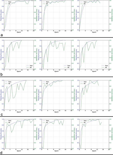
Figure 4. Training curves comparing a different set of four architectures using proposed entropy-based method.

Sub-figures (a) VGG19, (b) ResNet-18, (c) ResNet-34, (d) ResNet-50, demonstrating the performance of each architecture when utilizing the proposed entropy-based method for early stopping.

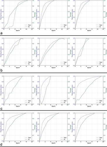
Figure 5. Training curves comparing a different set of four architectures using validation data based approach.

Sub-figures (a) RetiNet, (b) AOCT-NET, (c) DeepOCT, (d) Octnet, illustrating the performance of each architecture when utilizing a validation data based approach for early stopping.

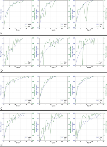
Figure 6. Training curves comparing a different set of four architectures using proposed entropy-based method.

Sub-figures (a) RetiNet, (b) AOCT-NET, (c) DeepOCT, (d) Octnet, demonstrating the performance of each architecture when utilizing the proposed entropy-based method for early stopping.

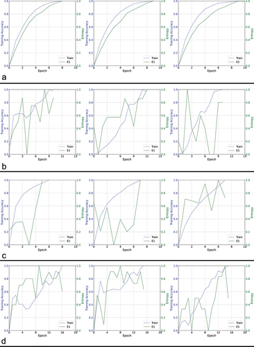
Figure 7. Comparing scatter and regression plots for final accuracy-epoch values in independent runs of architectures using both validation data-based and proposed entropy-based approaches.

Sub-figures (a) AlexNet, (b) VGG11, (c) VGG13, (d) VGG16, (e) VGG19, (f) ResNet-18, (g) ResNet-34, (h) ResNet-50, (i) RetiNet, (j) AOCT-NET, (k) DeepOCT, (l) Octnet dipict individual curves for both (1) validation data based approach and (2) the proposed entropy-based early stopping technique.

In the quantitative portion of our analysis, we identify, for each architecture under study, the run whose accuracy is closest to the mean accuracy of all thirty runs. From this identified run, we generate the confusion matrix and calculate Sensitivity, Specificity, Precision, and F1 scores for each class. Furthermore, we compute the average accuracy and the mean number of training epochs across all runs, providing a comprehensive view. These findings are consolidated in Table 1. For the statistical analysis, we initially evaluate the distribution of epoch values for each iteration to assess normality. This is performed using the Shapiro-Wilk test (Shapiro and Wilk 1965), under both configurations: with validation data and with the proposed early stopping method. Subsequently, the Kruskal-Wallis test (Hoffman 2019) is employed to scrutinize the statistical differences in the number of training epochs required when the proposed early stopping method is used, as compared to the traditional validation data approach. The threshold value for both tests is 0.05. The outcomes of these tests are collated in Table 2.

Table 1. Classification parameters with confusion matrix for different architectures using both validation data-based and proposed entropy-based approaches.

	Validation											Entropy
		CNV	DME	DRU	NOR	Sen	Spe	Pre	F1	Avg. Accuracy	Avg. Epoch	CNV	DME	DRU	NOR	Sen	Spe	Pre	F1	Avg. Accuracy	Avg. Epoch
	CNV	241	1	0	0	0.99	0.81	0.64	0.78			217	24	1	0	0.90	0.96	0.88	0.89
Alexnet	DME	11	230	1	0	0.95	0.96	0.89	0.92			1	240	1	0	0.99	0.93	0.83	0.90
	DRU	124	0	118	0	0.49	0.96	0.80	0.61			29	10	197	6	0.81	0.99	0.99	0.89
	NOR	0	25	2	189	0.78	1	1	0.88			0	14	0	228	0.94	0.99	0.97	0.96
										0.79	14.73									0.89	35.56
	CNV	226	4	12	0	0.93	0.99	0.99	0.96			238	3	1	0	0.98	0.99	0.97	0.97
VGG11	DME	2	238	2	0	0.98	0.99	0.98	0.98			4	237	0	1	0.98	0.99	0.98	0.98
	DRU	0	0	242	0	1	0.97	0.92	0.96			5	0	236	1	0.97	0.99	0.97	0.97
	NOR	0	1	7	234	0.97	1	1	0.98			0	1	5	236	0.97	1	0.99	0.98
										0.96	15.4									0.97	6.5
	CNV	238	4	0	0	0.98	0.99	0.97	0.97			232	10	0	0	0.96	0.99	0.99	0.97
VGG13	DME	2	240	0	0	0.99	0.99	0.97	0.98			2	240	0	0	0.99	0.98	0.95	0.97
	DRU	4	0	238	0	0.98	0.99	0.97	0.97			0	0	242	0	1	0.99	0.98	0.99
	NOR	0	4	8	230	0.95	1	1	0.97			0	3	4	235	0.97	1	1	0.98
										0.97	14.93									0.98	7.4
	CNV	231	5	6	0	0.95	0.99	0.99	0.97			233	9	0	0	0.96	0.99	0.98	0.97
VGG16	DME	2	240	0	0	0.99	0.99	0.97	0.98			1	241	0	0	0.99	0.99	0.96	0.98
	DRU	0	0	242	0	1	0.98	0.96	0.98			3	0	237	2	0.98	1	1	0.99
	NOR	0	3	5	234	0.97	1	1	0.98			0	0	0	242	1	1	0.99	0.99
										0.97	17.9									0.97	8.7
	CNV	232	9	1	0	0.96	0.99	0.98	0.97			236	5	1	0	0.98	0.98	0.96	0.96
VGG19	DME	0	242	0	0	1	0.98	0.95	0.97			0	241	0	1	1	0.99	0.98	0.99
	DRU	3	0	239	0	0.98	0.99	0.98	0.99			11	0	231	0	0.95	1	0.99	0.97
	NOR	0	2	2	238	0.98	1	1	0.99			0	1	0	241	0.99	1	0.99	0.99
										0.98	18.87									0.98	11.67
	CNV	241	1	0	0	0.99	0.95	0.87	0.93			232	8	0	2	0.96	0.97	0.90	0.93
ResNet-18	DME	12	230	0	0	0.95	0.99	0.99	0.97			2	239	0	1	0.99	0.99	0.96	0.97
	DRU	24	0	218	0	0.90	0.97	0.92	0.91			23	0	218	1	0.90	0.99	0.99	0.94
	NOR	0	1	19	222	0.92	1	1	0.96			0	2	2	238	0.98	0.98	0.98	0.98
										0.94	11.76									0.96	6.2
	CNV	232	9	1	0	0.96	0.99	0.99	0.97			222	13	7	0	0.92	1	1	0.96
ResNet-34	DME	0	242	0	0	1	0.98	0.96	0.98			0	241	1	0	0.99	0.98	0.94	0.96
	DRU	3	0	239	0	0.99	0.99	0.99	0.99			0	0	242	0	1	0.96	0.90	0.94
	NOR	0	2	2	238	0.98	1	1	0.99			0	3	22	217	0.90	0.99	0.96	0.94
										0.95	15.13									0.95	9.97
	CNV	232	2	1	1	0.98	0.96	0.90	0.94			222	13	7	0	0.92	1	1	0.96
ResNet-50	DME	2	236	0	4	0.97	0.99	0.99	0.98			0	240	1	1	0.99	0.98	0.94	0.96
	DRU	24	0	205	13	0.85	0.99	0.99	0.91			0	0	242	0	1	0.96	0.89	0.94
	NOR	0	0	0	242	1	0.95	0.93	0.96			0	3	22	217	0.90	1	0.99	0.94
										0.94	16.13									0.90	10.1
	CNV	231	11	0	0	0.95	0.96	0.88	0.92			234	5	3	0	0.97	0.99	0.99	0.98
AOCT-NET	DME	0	235	0	7	0.97	0.98	0.95	0.96			3	218	1	20	0.90	0.99	0.98	0.94
	DRU	30	0	204	8	0.84	0.99	0.99	0.91			0	0	237	5	0.98	0.99	0.98	0.98
	NOR	0	0	1	241	0.99	0.98	0.94	0.97			0	0	1	241	0.99	0.97	0.96	0.95
										0.94	24.13									0.96	16.3
	CNV	228	10	4	0	0.94	0.99	0.98	0.96			226	14	2	0	0.93	0.99	0.98	0.96
RetiNet	DME	1	231	4	6	0.95	0.98	0.96	0.95			2	234	1	5	0.97	0.98	0.94	0.95
	DRU	3	0	238	1	0.98	0.98	0.94	0.96			3	0	239	0	0.99	0.99	0.96	0.98
	NOR	0	0	7	235	0.97	0.99	0.97	0.97			0	1	6	235	0.97	0.99	0.98	0.98
										0.96	11.56									0.96	10.46
	CNV	236	3	3	0	0.97	0.97	0.91	0.94			235	6	1	0	0.97	0.98	0.94	0.95
DeepOCT	DME	13	219	0	10	0.90	0.99	0.98	0.94			3	231	1	7	0.95	0.99	0.96	0.96
	DRU	9	0	228	5	0.94	0.99	0.97	0.96			13	3	218	8	0.90	0.99	0.99	0.94
	NOR	0	2	3	237	0.98	0.98	0.94	0.96			0	1	1	240	0.99	0.98	0.94	0.96
										0.95	18.93									0.95	7.9
	CNV	238	4	0	0	0.98	0.97	0.91	0.94			228	14	0	0	0.94	0.98	0.95	0.95
Octnet	DME	3	228	1	10	0.94	0.99	0.98	0.96			1	239	0	2	0.99	0.97	0.93	0.96
	DRU	21	0	217	4	0.90	0.99	0.99	0.94			11	0	231	0	0.95	0.99	0.99	0.97
	NOR	0	0	1	241	0.99	0.98	0.94	0.97			0	5	1	236	0.97	0.99	0.99	0.98
										0.95	24.57									0.96	23.5

Table 2. Statistical testing.

	Shapiro – Wilk Test (Validation)	Shapiro – Wilk Test (Entropy)	Kruskal-Wallis Test
Alexnet	0.178	0.022	6.492 × 10^−11
VGG11	0.001	0.002	2.101 × 10^−11
VGG13	0.112	8.502 × 10^−4	2.274 × 10^−11
VGG16	8.543 × 10^−4	0.001	2.335 × 10^−11
VGG19	0.176	0.053	3.608 × 10^−5
RES18	0.143	6e-4	2.420 × 10^−11
RES34	0.858	0.253	8.073 × 10^−6
RES50	0.535	0.182	1.898 × 10^−10
AOCT-NET	0.610	2.209 × 10^−6	1.248 × 10^−7
RetiNet	2.036 × 10^−4	0.175	5.161 × 10^−3
DeepOCT	3.225 × 10^−4	1.676 × 10^−3	2.110 × 10^−11
OctNet	0.273	0.026	0.477

Discussion

In our tests, we observed that the entropy (E1) curve generally exhibits a monotonically increasing function among the different test CNN architectures, with exceptions observed in OCT-specific network architectures other than RetiNet (Figure 6). However, the validation accuracy curve for OCT-specific architectures is not smooth either (Figure 5). Therefore, the roughness in the entropy (E1) curve can be attributed to the network architecture. The monotonic increase in the entropy curves enables more accessible monitoring of the network’s training progress without requiring a specific termination condition when local maxima occur due to abrupt changes. The implementation is straightforward and does not necessitate a patience factor. Additionally, the nearly uniform rate of change in the entropy curve allows for a 1:1 mapping with the training state, which can help estimate the proportion of training that will be completed within a given time frame when the estimated execution time is known. Despite the uneven shape of these curves, the overall trend across epochs is increasing, indicating that entropy remains a suitable metric for tracking the network’s progress. In cases where the entropy curve is not smooth, a small constant $({\alpha }_0)$ is needed to ensure the network does not terminate prematurely. Although the irregular curve makes monitoring more challenging, it is unlikely to affect the overall accuracy, as the curve does eventually reach maxima and terminate. This observation is further supported by the accuracy values presented in Table 1. We analyzed every accuracy-epoch pair value from several iterations of the algorithms with varying learning rates, presenting them as scatter plots with regression lines to examine the overall trend, and as histograms to visualize the distribution of values. In Figure 7, the histograms show that, except for AlexNet and Octnet, the values corresponding to the proposed method are skewed to the left, indicating an overall reduction in the number of training epochs required. Moreover, the proposed entropy approach results in a smaller dispersion of values in terms of accuracy, except for ResNet-34, RetiNet, and Octnet, where the spread is similar to when validation data is used. The overall trend, as observed through regression lines, reveals that the proposed method maintains a similar trend to when validation data is used, except in the case of VGG13, VGG19, ResNet-50, and Octnet. However, except for VGG19 and ResNet-50, the difference in trend is acceptable, as the trend in other networks using the proposed method is increasing, while the existing validation data-based approach shows a decrease in accuracy with increasing epochs. Based on these observations, the proposed methodology is overall more effective than the existing validation data-based approach.

Quantitative Analysis

The actual label and classifier output is positive in True Positive (TP) cases. False Positive (FP) occurs when the real label is negative, yet the classifier’s output is positive. False Negative (FN) occurs when the real label is positive, yet the classifier’s result is negative. True Negative (TN) situations occur when both the output of the classifier and the actual label are negative.

(14) $\mathrm{Precision}=\frac{\mathit{TP}}{\mathit{TP}+\mathit{FP}}$(14)

(15) $\mathrm{Sensitivity}/\mathrm{Recall}=\frac{\mathit{TP}}{\mathit{TP}+\mathit{FN}}$(15)

(16) $\mathrm{Specificity}=\frac{\mathit{TN}}{\mathit{TN}+\mathit{FP}}$(16)

(17) $\mathrm{F}1-\mathrm{Score}=\frac{2\ast \mathrm{Precision}\ast \mathrm{Recall}}{\mathrm{Precision}+\mathrm{Recall}}$(17)

Precision quantifies the number of accurate positive predictions, whereas Recall, also known as Sensitivity, quantifies the proportion of accurate positive predictions among all positive forecasts. The F1-Score is the harmonic mean of the Precision and Recall measures. Specificity, or the true negative rate (TNR), evaluates the capacity to determine healthy cases correctly. In a classification problem with several classes, values must be computed independently for each class. However, accuracy can be used to compare all classes using a single metric. The classification model contains four categories, including disease classes for CNV, DME, and Drusen and a separate healthy class. The confusion matrix compares the output of the model derived from test data to the actual test labels in a $\mathit{n}$ x $\mathit{n}$ matrix, where $\mathit{n}$ is the number of classes. Since our model includes four classes, the confusion matrix’s dimensions are 4 × 4. The confusion matrix comprehensively studies the classification model due to its class-by-class comparison. After determining the algorithm iteration that is closest to the mean accuracy across multiple iterations, the confusion matrix is constructed. Sensitivity (Sen), specificity (Spe), precision (Pre), and the F1 score are calculated separately for each class in the dataset. Comparing the proposed entropy technique to the method based on validation data, along with the average accuracy and the average number of training iterations, the values for each architecture are listed separately (Table 1).

As evidenced in Table 1, there is a reduction in training epochs in all cases except AlexNet, and an increase in average accuracy in all instances except ResNet-50. Given that ResNet-50 has a greater number of layers than the other architectures in the study, it is plausible to deduce that the larger number of layers could be one of the contributing factors to the observed decrease in accuracy. In other evaluated networks, the gain in accuracy is either limited or similar to the traditional validation data-based approach. However, this minor limitation does not overshadow our main objective, which is to present an alternative to using validation data for early stopping, with the added benefit of reducing the number of epochs needed for training. Therefore, despite some variations, our proposed methodology provides a more efficient solution.

Statistical Analysis

In our study, we conducted two different statistical tests with a standard threshold p-value of 0.05. The results of these tests are presented in Table 2. Since each network was run thirty times, we had thirty data points available for statistical analysis. We initially employed the Shapiro-Wilk test to assess the normality of the distribution of epoch values across the different learning rates used in our study. Under the existing validation data-based method for early stopping, epoch values generally followed a normal distribution, with exceptions noted for VGG11, VGG16, RetiNet, and Octnet. However, when using our proposed entropy-based method, a non-normal distribution was observed, except for VGG19, ResNet-34, ResNet-50, and Retinet.

The normal distribution observed in the existing validation data-based method for early stopping suggests that the number of epochs required for training is consistent and predictable for most of the learning rates studied, except for VGG11, VGG16, RetiNet, and Octnet. This consistency and predictability can be advantageous in settings with limited computational resources or time constraints, as it provides a clear expectation for the computational costs involved in training the model. On the other hand, the non-normal distribution observed in the proposed entropy-based method implies a variability in the number of epochs required for training across different learning rates. While this may seem less predictable, it potentially indicates a more flexible approach that adapts to the specific requirements of different learning rates. This adaptability could lead to more efficient training, especially in cases where a learning rate that would typically require a high number of epochs can be trained with fewer epochs using the entropy-based method. In essence, the non-normal distribution in the proposed method may be an indication of its adaptability and efficiency across diverse learning rates, while the normal distribution in the existing method indicates its predictability and consistency across different learning rates.

The Kruskal-Wallis test, a non-parametric method, was used to compare the median number of training epochs between the existing validation data-based method and the proposed entropy-based method. Except for the Octnet architecture, our research discovered a significant difference in all other instances. This suggests that, for most architectures, the number of training epochs required by the proposed entropy-based method differs from that required by the currently used validation data-based method. Specifically, the significant Kruskal-Wallis results indicate the potential efficacy of the proposed entropy-based method, as it generally requires fewer training epochs across most architectures. For the Octnet architecture, where no significant difference was found, this indicates that the proposed entropy-based method does not significantly affect the number of training epochs compared to the existing validation data-based method. This may be due to particular characteristics of the Octnet architecture or its interaction with various learning rates.

Conclusion

The entropy-based deep neural network training optimization technique proposed in this paper offers a compelling alternative to the traditional validation data-based early stopping method, demonstrating efficiency and adaptability across various deep learning architectures. The technique effectively reduces the required training epochs while enhancing model accuracy. The proposed technique presents an independent monitoring system that effectively addresses potential bias concerns associated with the size of the validation dataset or the distribution of classes. Simultaneously, given the nature of our methodology, it remains unaffected by the dataset, thereby exhibiting a restricted reliance on the data quality. The implementation of the proposed technique is straightforward and does not necessitate any modifications to the optimizer or the loss function; this guarantees that the training of the network remains unaffected. The data flow remains unaltered, as the proposed training technique does not entail any modifications to the underlying network architecture. The proposed technique solely focuses on the monitoring of the weights. Hence, if the network goes out of bounds, it will remain undetected. With the exception of the ResNet-50 architecture, there was an observed increase in accuracy ranging from 0.28% to 12.66%. Furthermore, there was a notable reduction in training epochs required, varying from 4.35% to 58.27%, with the exception of Alexnet. Through the Shapiro-Wilk test, it was observed that the epoch value distribution with the conventional method followed a normal distribution, except for VGG11, VGG16, RetiNet, and Octnet, while with the proposed technique, the trend veered toward a non-normal distribution, except in the cases of VGG19, ResNet-34, ResNet-50, and Retinet. The Kruskal-Wallis test further substantiated these observations, revealing a significant difference in epoch values between the two methods for all architectures except Octnet. Despite these exceptions, the proposed technique’s potential is apparent, particularly where computational resources or time are limited. The proposed technique assumes the presence of at least one multi-node fully connected layer. The proposed methodology will not be applicable if the architecture has only one fully connected layer with a single node.

Disclosure Statement

No potential conflict of interest was reported by the author(s).

Data Availability Statement

The data that support the findings of this study are openly available in ’Mendeley Data’ at http://doi.org/10.17632/rscbjbr9sj.2_oct_2017_data.

References

- Alqudah, A. M. 2020. AOCT-NET: A convolutional network automated classification of multiclass retinal diseases using spectral-domain optical coherence tomography images. Medical & Biological Engineering & Computing 58 (1):41–25. doi:10.1007/s11517-019-02066-y
- Altan, G. 2022. DeepOCT: An explainable deep learning architecture to analyze macular edema on OCT images. Engineering Science and Technology, an International Journal 34:101091. doi:10.1016/j.jestch.2021.101091
- Apostolopoulos, S., C. Ciller, S. De Zanet, S. Wolf, and R. Sznitman. 2017. RetiNet: Automatic AMD identification in OCT volumetric data. Investigative Ophthalmology & Visual Science 58 (8):387–387.
- Bai, Y., E. Yang, B. Han, Y. Yang, J. Li, Y. Mao, G. Niu, and T. Liu. 2021. Understanding and improving early stopping for learning with noisy labels. Advances in Neural Information Processing Systems 34:24392–403.
- Bonet, D., A. Ortega, J. Ruiz-Hidalgo, and S. Shekkizhar. 2021. Channel-wise early stopping without a validation set via NNK polytope interpolation. arXiv preprint arXiv:2107.12972.
- Brownlee, J. 2020. Understand the impact of learning rate on neural network performance. Accessed September 3 2021. https://machinelearningmastery.com/understand-the-dynamics-of-learning-rate-on-deep-learning-neural-networks/
- Bu, Y., S. Zou, and V. V. Veeravalli. 2020. Tightening mutual information-based bounds on generalization error. IEEE Journal on Selected Areas in Information Theory 1 (1):121–30. doi:10.1109/JSAIT.2020.2991139
- Duvenaud, D., D. Maclaurin, and R. Adams. 2016. Early Stopping as Nonparametric Variational Inference. In Proceedings of the 19th International Conference on Artificial Intelligence and Statistics, ed. A. Gretton and C. C. Robert, 1070–1077. Cadiz, Spain: Proceedings of Machine Learning Research (PMLR).
- Forouzesh, M., and P. Thiran. 2021. “Disparity between batches as a signal for early stopping.” In Machine Learning and Knowledge Discovery in Databases. Research Track: European Conference, ECML PKDD 2021, Bilbao, Spain, September 13–17, 2021, Proceedings, Part II 21, 217–32. Springer.
- Gu, J., Z. Wang, J. Kuen, L. Ma, A. Shahroudy, B. Shuai, T. Liu, X. Wang, G. Wang, J. Cai, et al. 2018. Recent advances in convolutional neural networks. Pattern Recognition 77:354–77. doi:10.1016/j.patcog.2017.10.013
- He, K., X. Zhang, S. Ren, and J. Sun. 2016. Deep residual learning for image recognition. In Proceedings of the IEEE conference on computer vision and pattern recognition, June 26 - July 1, Las Vegas, Nevada, 770–78.
- Hoffman, J. I. E. 2019. Chapter 25 - analysis of variance. I. One-way. In Basic biostatistics for medical and biomedical practitioners, ed. J. I. E. Hoffman, 391–417. 2nd ed. London: Academic Press.
- Irsch, K. 2021. Optical principles of OCT. In Albert and Jakobiec’s principles and practice of ophthalmology, ed. Daniel M. Albert, Joan W. Miller, Dimitri T. Azar and Lucy H. Young, 1–14. Springer Nature Switzerland AG: Springer.
- Janocha, K., and W. M. Czarnecki. 2017. On loss functions for deep neural networks in classification. CoRR abs/1702.05659. http://arxiv.org/abs/1702.05659
- Karthik, K., and M. Mahadevappa. 2023. Convolution neural networks for optical coherence tomography (OCT) image classification. Biomedical Signal Processing and Control 79:104176. doi:10.1016/j.bspc.2022.104176
- Kermany, D. S., M. Goldbaum, W. Cai, C. C. Valentim, H. Liang, S. L. Baxter, A. McKeown, G. Yang, X. Wu, F. Yan, et al. 2018. Identifying medical diagnoses and treatable diseases by image-based deep learning. Cell 172(5):1122–31.e9. doi:10.1016/j.cell.2018.02.010
- Kermany, D., K. Zhang, and M. Goldbaum. 2018. Labeled optical coherence tomography (OCT) and chest X-ray images for classification (2018). Mendeley Data V2. doi:10.17632/rscbjbr9sj.2
- Krizhevsky, A., I. Sutskever, and G. E. Hinton. 2012. Imagenet classification with deep convolutional neural networks. Advances in Neural Information Processing Systems 25: 1097–105.
- Lindsay, G. W. 2021. Convolutional neural networks as a model of the visual system: Past, present, and future. Journal of Cognitive Neuroscience 33 (10):2017–31. doi:10.1162/jocn_a_01544
- Liu, K., R. Ali Amjad, and B. C. Geiger. 2018. Understanding individual neuron importance using information theory. arXiv Preprint arXiv: 1804.06679.
- Liu, Y., J. A. Starzyk, and Z. Zhu. 2008. Optimized approximation algorithm in neural networks without overfitting. IEEE Transactions on Neural Networks 19 (6):983–95. doi:10.1109/TNN.2007.915114
- Li, T., Z. Zhuang, H. Liang, L. Peng, H. Wang, and J. Sun. 2021. Self-validation: Early stopping for single-instance deep generative priors. arXiv Preprint arXiv: 2110.12271.
- Mahsereci, M., L. Balles, C. Lassner, and P. Hennig. 2017. Early stopping without a validation set. arXiv Preprint arXiv: 1703.09580.
- Narkhede, M. V., P. P. Bartakke, and M. S. Sutaone. 2022. A review on weight initialization strategies for neural networks. Artificial Intelligence Review 55 (1):291–322. doi:10.1007/s10462-021-10033-z
- Park, E., J. Ahn, and S. Yoo. 2017. Weighted-entropy-based quantization for deep neural networks. In Proceedings of the IEEE Conference on Computer Vision and Pattern Recognition, Honolulu, Hawaii, 5456–64.
- Pinto, T., H. Morais, and J. M. Corchado. 2019. Adaptive entropy-based learning with dynamic artificial neural network. Neurocomputing 338:432–40. doi:10.1016/j.neucom.2018.09.092
- Podoleanu, A. G. 2012. Optical coherence tomography. Journal of Microscopy 247 (3):209–19. doi:10.1111/j.1365-2818.2012.03619.x
- Powers, D. M. 2020. Evaluation: From precision, recall and F-measure to ROC, informedness, markedness and correlation. arXiv Preprint arXiv: 2010.16061.
- Raskutti, G., M. J. Wainwright, and B. Yu. 2014. Early stopping and non-parametric regression: An optimal data-dependent stopping rule. The Journal of Machine Learning Research 15 (1):335–66.
- Rawat, W., and Z. Wang. 2017. Deep convolutional neural networks for image classification: A comprehensive review. Neural Computation 29 (9):2352–449. doi:10.1162/neco_a_00990
- Shannon, C. E. 1948. A mathematical theory of communication. The Bell System Technical Journal 27 (3):379–423. doi:10.1002/j.1538-7305.1948.tb01338.x
- Shapiro, S. S., and M. B. Wilk. 1965. An analysis of variance test for normality (complete samples). Biometrika 52 (3/4):591–611. doi:10.1093/biomet/52.3-4.591
- Silva, L. M., J. M. de Sá, and L. A. Alexandre. 2005. Neural network classification using Shannon’s entropy. In Esann, 217–222. Citeseer.
- Simonyan, K., and A. Zisserman. 2014. Very deep convolutional networks for large-scale image recognition. arXiv Preprint arXiv: 14091556.
- Sinha, A., M. Sarkar, A. Mukherjee, and B. Krishnamurthy. 2017. Introspection: Accelerating neural network training by learning weight evolution. arXiv Preprint arXiv: 1704.04959.
- Srinivasan, V., C. Eswaran, and N. Sriraam. 2007. Approximate entropy-based epileptic EEG detection using artificial neural networks. IEEE Transactions on Information Technology in Biomedicine 11 (3):288–95. doi:10.1109/TITB.2006.884369
- Steinke, T., and L. Zakynthinou. 2020. Reasoning about generalization via conditional mutual information. In Conference on Learning Theory, Graz, Austria, 3437–52. PMLR.
- Sunija, A. P., S. Kar, S. Gayathri, V. P. Gopi, and P. Palanisamy. 2021. Octnet: A lightweight cnn for retinal disease classification from optical coherence tomography images. Computer Methods and Programs in Biomedicine 200:105877. doi:10.1016/j.cmpb.2020.105877
- Vardasbi, A., M. de Rijke, and M. Dehghani. 2022. Intersection of Parallels as an Early Stopping Criterion. In Proceedings of the 31st ACM International Conference on Information & Knowledge Management, Atlanta,GA, USA, 1965–74.
- Xu, Y., P. Cao, Y. Kong, and Y. Wang. 2019. L_dmi: A novel information-theoretic loss function for training deep nets robust to label noise. Advances in Neural Information Processing Systems 32.
- Xu, A., and M. Raginsky. 2017. Information-theoretic analysis of generalization capability of learning algorithms. Advances in Neural Information Processing Systems 30.
- Yilmaz, A., and R. Poli. 2022. Successfully and efficiently training deep multi-layer perceptrons with logistic activation function simply requires initializing the weights with an appropriate negative mean. Neural Networks 153:87–103. doi:10.1016/j.neunet.2022.05.030