Generation of Vessel Track Characteristics Using a Conditional Generative Adversarial Network (CGAN)

ABSTRACT

Machine learning (ML) models often require large volumes of data to learn a given task. However, access and existence of training data can be difficult to acquire due to privacy laws and availability. A solution is to generate synthetic data that represents the real data. In the maritime environment, the ability to generate realistic vessel positional data is important for the development of ML models in ocean areas with scarce amounts of data, such as the Arctic, or for generating an abundance of anomalous or unique events needed for training detection models. This research explores the use of conditional generative adversarial networks (CGAN) to generate vessel displacement tracks over a 24-hour period in a constraint-free environment. The model is trained using Automatic Identification System (AIS) data that contains vessel tracking information. The results show that the CGAN is able to generate vessel displacement tracks for two different vessel types, cargo ships and pleasure crafts, for three months of the year (May, July, and September). To evaluate the usability of the generated data and robustness of the CGAN model, three ML vessel classification models using displacement track data are developed using generated data and tested with real data.

Introduction

The movement of vessels through both national and international waters are of interest to both security and defense personnel. In international waters, vessel monitoring takes place for the benefit of the environment, safety, and the defense and security of national jurisdictions. In national waters, the motivation behind vessel monitoring is expanded to include protection of natural habitats, enforcement of national shipping regulations, collision avoidance, etc. In general terms, more constraints are added to vessel movement within a nation’s water space.

Vessel movement constraints are environmental (e.g., coastline, ice, ship density), vessel-based (e.g., maximum speed, fuel capacity), and regulatory (e.g., speed regulations, shipping lanes). As well, depending on the specific constraint, violating the constraint will result in different consequences. The lower end of the consequence scale would include a warning from an authority to reduce vessel speed. The upper end of the consequence scale could involve the grounding or sinking of a vessel due to an impact with the coastline or an underwater obstacle.

Some national waters have an abundance of physical hazards that produce constraints. As well, the opening of new potential waterways adds to the complexity of vessel movement, as these waterways often have old or incomplete charts. An example is the Canadian Arctic, where the intricate physical characteristics of the land mass are combined with the moving constraint of ice.

As vessel traffic is introduced into the waterways of the Canadian Arctic, it is important to combine modern monitoring capabilities with modern vessel predictive techniques. For example (Campbell, Isenor, and Dais Ferreira 2022), used machine learning (ML) to successfully identify a large group of fabricated vessels that were reported to be crossing the Atlantic. Although ML can be considered predictive in terms of classification, ML does require a sizable amount of high quality (i.e., clean) data. This means modern analysis approaches (e.g., ML) need to be supported with an information infrastructure that can provide high quality data (Syms et al. 2021).

Access to large, diverse, and annotated data sets¹ represents another challenge to using ML. Annotations are a problem as they often are assigned by humans which is a time-consuming process. However, generated data are automatically annotated when created, which avoids the labeling issue. In this paper, we use a form of generative Artificial Intelligence (AI), called a conditional generative adversarial network (CGAN) (Mirza and Osindero 2014) to generate vessel displacement tracks using Automatic Identification System (AIS) data.² The displacement track, which is the shortest path of a vessel between its first and last position of the day, is considered preliminary progress toward the generation of more complete and complex vessel tracks under constraints. The conditional model is used in this work as a method to isolate the statistical characteristics of a specific vessel type.

Generative Adversarial Networks and Related Work

In 2014, generative adversarial networks (GANs) were introduced by Goodfellow et al. (2014). as a form of generative AI used to create synthetic data values. A GAN consists of two neural networks, the discriminator (D) and the generator (G) that compete in an adversarial setting (Campbell, Ferreira, and Isenor 2023). A GAN can produce a large volume of generated data with minimal effort. Generated data can be used to improve data quality, enhance scalability, help remove bias, up-sample rare events to improve diversity, and address privacy issues associated with granting access to data (Campbell, Ferreira, and Isenor 2023).

Since the introduction of GANs, there have been promising applications in the field of image generation (thispersondoesnotexist.com Accessed: 2024) (Bao et al. 2017; Zhang et al. 2022),; text-text generation (OpenAI:Chatgpt Accessed: 2024b) (Chen et al. 2020; Li et al. 2023),; and text-image generation (OpenAI:Dalle 2024a) (Liao et al. 2022; Tao et al. 2022); that has fueled research toward developing and evolving the architectures and applications of GANs. As a result, many adaptations to the original GAN architecture have developed including Deep Convolutional GAN (Radford, Metz, and Chintala 2016), CGAN (Mirza and Osindero 2014), Wasserstein GAN (Arjovsky, Chintala, and Bottou 2017), InfoGAN (Chen et al. 2016), etc.

GANs have also been used for various tasks related to the generation and imputation of missing values in a wide variety of data sets. This includes application to medical records and historical air quality data (Yonghong et al. 2018), as well as, traffic flow data, basketball player trajectories, and billiard ball trajectories (Lui, et al. 2019). GANs have been used to model and generate classical music (Mogren 2016), real-value medical data (Esteban, Hyland, and Rätsch 2017), and stock prices and energy data (Yoon, Jarrett, and van der Schaar 2019).

Considering spatio-temporal data, a review by Gao, et al (Nan et al. 2022). indicates the considerable depth of spatio-temporal GANs applications including in the areas of time series, trajectories, spatio-temporal events, and spatio-temporal graphs. In topics related to trajectories of objects, GANs have been used to model and predict pedestrian trajectories and interactions (Gupta et al. 2018; Kosaraju et al. 2019; Liu et al. 2020; Sadeghian et al. 2019), taxi hot-spots (Yu et al. 2020), and crime related events for security and protection (Jin et al. 2019).

Specific to the movement of maritime vessels, GANs have been used to generate several minutes of missing positions in a vessel trajectory (Zhang et al. 2023). As well, the handling behavior of a vessel has been predicted using a GAN (Gao and Shi 2020) for the purpose of collision avoidance. In the current literature, the research focuses on augmenting the track of an existing vessel. To the best of our knowledge, generating vessel trajectories for non-existent ships using GANs is still an open area to be investigated and is explored in this piece of work.

In the application of constraints within a GAN, work has been done on pedestrian trajectory prediction while considering stationary and mobile obstacles (Sadeghian et al. 2019). For vessels, trajectory prediction within a channel has been considered using a repulsive potential field method (Lu et al. 2023). Specific to Liang et. al (Liang et al. 2024) is the introduction of spatial and temporal correction, which is relevant to the vessel positional data used in this study. Although spatial correlations have not been incorporated in the current work, such correlations do exist in vessel data. These correlations result from report-to-report relationships for a single vessel and vessel-to-vessel relationships in well-defined vessel traffic routes (McArthur and Isenor 2021).

Motivation and Contributions

The ultimate goal of this work is the generation of realistic vessel tracks for the Canadian Arctic that considers the constraints of the intricate coastline and ice conditions. The vessel tracks will be used for algorithm testing related to defense and security monitoring. This paper represents a step toward this goal, with the establishment of an operating GAN that generates realistic daily positions of vessels without accounting for environmental, vessel-based, and regulatory constraints.

The contributions of this work include:

• the application of a GAN to geospatial vessel movement data in an area of complex shoreline;

• investigation of the realism of generated vessel positions using sparse input data, such as would exist in the Arctic;

• the generation of representative features for vessel displacement tracks for two different vessel types;

• a comprehensive evaluation of the model performance using loss curves, column shapes, correlation measures, boundary adherence, and new row synthesis;

• the evaluation of the proposed model using machine learning efficacy tests that show that the use of generated data is promising for the development of vessel models deployed in a real-world setting; and

• showing the robustness of the model by generating data for different times of the year.

The paper is structured as follows. Section 2 describes how GANs and CGANs are trained to generate synthetic data. Section 3 discusses the data set and model architectures used to perform the generation of vessel displacement tracks. Section 4 covers the results of the generation process and discusses the outcome and evaluation of all the generated data. Lastly, Section 5 summarizes the conclusions and discusses the future work.

Conditional Generative Adversarial Networks

GANs were first introduced as a form of generative modeling used to create synthetic data samples that resemble or mimic real data. The CGAN is an adaptation of the original GAN framework that incorporates conditional information into the training process. This section will discuss the architecture and training process associated with the original GAN framework and then cover how the condition information is incorporated to create the CGAN.

Original GAN Framework

The original GAN framework consists of two neural networks that compete with one another in an adversarial setting with opposing objectives. The networks compete in a zero-sum game where the loss of one network is the other’s gain and vice versa (Saxena and Cao 2021). The two networks that make up the architecture of the GAN are the $\mathcal{G}$ and $\mathcal{D}$. The goal of each network is as follows:

• $\mathcal{D}$: the $\mathcal{D}$ receives both real and synthetic data as input and estimates the probability that a data instance came from the real data class. The goal of the $\mathcal{D}$ is to correctly classify a data point as real or generated.

• $\mathcal{G}$: the $\mathcal{G}$ creates synthetic data from random noise that captures and mimics the distribution of the real data. The goal of the $\mathcal{G}$ is to create data that fools the $\mathcal{D}$ into believing it is real.

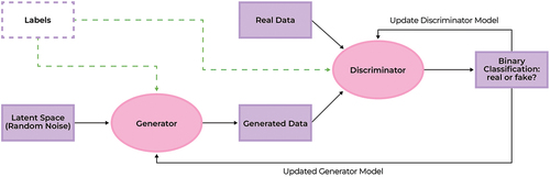
Figure 1 illustrates the original GAN architecture (solid lines only). The training process starts with random noise being fed into the $\mathcal{G}$ where synthetic data samples are created. These data are then fed into the $\mathcal{D}$ alongside real data where the $\mathcal{D}$ must classify each instance as real or generated. The $\mathcal{D}$ outputs a scalar value that represents the probability that the data point is from the real data distribution. The probabilities for the real and generated data are combined into a value function for the GAN, given below:

(1) $E_{\mathit{X}\sim {\mathit{p}}_{\mathit{data}}}[log(\mathit{D}(\mathit{X}))]+E_{Z\sim p_Z}[log(1-\mathit{D}(\mathit{G}(\mathit{Z})))]$(1)

Figure 1. The depiction of the GAN architecture is represented by the solid lines. When the purple and green dotted lines are taken into consideration the diagram represents the structure of a CGAN.

This can be generalized into more common probability theory notation as:

(2) $E_X[{log}_2(D_{\theta }(\mathit{X}))]+E_Z[{log}_2(1-D_{\theta }(\mathit{G}(\mathit{Z})))]$(2)

where $E_X/E_Z$ is the expected value over real $(\mathit{X})$/random noise $(\mathit{Z})$ samples, $D_{\theta }(\mathit{X})$ is the $\mathcal{D}$’s probability that a real instance is real, $\mathit{G}(\mathit{Z})$ is the $\mathcal{G}$ output for a generated sample created from random noise, $D_{\theta }(\mathit{G}(\mathit{Z}))$ is the $\mathcal{D}$’s probability that a generated instance is real, $\mathit{\theta }$ are the hyperparameters that define the $\mathcal{D}$, and $1-D_{\theta }(\mathit{G}(\mathit{Z}))$ is the probability that a generated instance is generated.

The value function above is then used to define an objective function. The objective function is based on a game theory concept that involves the “simultaneous” optimization of both the $\mathcal{G}$ and $\mathcal{D}$ networks (Campbell, Ferreira, and Isenor 2023). As a result, each network competes to maximize its probability of “winning” this adversarial game. The goal of the $\mathcal{G}$ is to minimize the value function as it wants to reduce the number of generated data points being assigned a low probability by the $\mathcal{D}$. In contrast, the $\mathcal{D}$’s goal is to maximize the number of generated data points being assigned a low probability, and maximize the number of real data points being assigned a high probability. This will occur when the value function is maximized.

To train both networks, independent backpropagation procedures are performed (Nielsen 2015). Backpropagation depends on the loss calculation which is computed using binary cross entropy in this study. The loss compares the actual outcome to the predicted outcome to assess the error of the model output, which is then used to adjust the values of the model parameters. This training process continues until a balance is reached where the $\mathcal{G}$ creates realistic data and the $\mathcal{D}$ cannot easily identify the synthetic data from the real data. The training process aims to find the Nash equilibrium (Hazra and Anjaria 2022), where the $\mathcal{G}$ and $\mathcal{D}$ reach a state where neither can improve significantly without the other changing.

Conditional GAN

The conditional GAN extends the capability of the original GAN framework by incorporating conditional information into the training process for both the $\mathcal{G}$ and $\mathcal{D}$. This extra information can be a label or data from other modalities which are fed into $\mathcal{G}$ and $\mathcal{D}$ as part of the input (Mirza and Osindero 2014). This condition is fed into the $\mathcal{D}$ and $\mathcal{G}$ as part of the input as illustrated by the purple and green dotted lines in Figure 1. In the case of the condition being a class label, it would provide specific information to inform the $\mathcal{G}$ which class the synthetic data should mimic or resemble. For the $\mathcal{D}$, the particular class preconditions the $\mathcal{D}$ before it assesses if the data point is real or synthetic. Figure 1 shows how this conditional information is fed into a CGAN via the dotted lines.

In a CGAN the value function used to evaluate the samples is now defined as (Mirza and Osindero 2014):

(3) $E_X[{log}_2(D_{\theta }(\mathit{X}|\mathit{Y}))]+E_Z[{log}_2(1-D_{\theta }(\mathit{G}(\mathit{Z}|\mathit{Y})))]$(3)

where $\mathit{Y}$ is the predefined condition. The value function now incorporates both the adversarial aspect of detecting real from generated, as well as the predefined condition. The CGAN is trained in the same manner as the GAN described in Section 2.1.

The benefit to using a conditional model is that this allows control of the modes or classes that the $\mathcal{G}$ creates. In the original GAN framework, the only method of incorporating a condition on the generated data is through the separate execution of the model for each vessel type. For this work, the choice of implementing a CGAN allows for an input condition, such as the vessel type, that limits the generated data to be applicable to that specific category of vessel. Therefore, the CGAN offers the flexibility of generating many vessel types or modalities within a single model.

The Experiment

This work investigates the use of CGANs for generating data that is representative of vessel displacement tracks in a constraint-free environment; i.e., the data generated are not required to adhere to any ship movement, environmental, or regulatory constraints.

The choice to use a GAN based architecture was made due to the model’s ability to generate diverse instances when very little data is available. Furthermore, the recent success of GAN based architectures in other applications of data generation (thispersondoesnotexist.com Accessed: 2024; OpenAI:Chatgpt Accessed: 2024b; OpenAI:Dalle 2024a) has shown remarkable success with convincing results. For this work, the CGAN was chosen so that different types of ship data could be generated using a single architecture.

The Data

The Automatic Identification System (AIS)³ data set used in this experiment was obtained from MarineCadastre.gov,⁴ which is an open and available source that provides ocean information, tools, and vessel traffic data. These AIS data are collected by the United States Coast Guard in both US and international waters. The data sets used for this work cover the months of May, July, and September of 2022 and is available at (NOAA 2024). The data files contain the following features: day, time, a vessel identifier called the Maritime Mobile Service Identity (MMSI), vessel latitude position, vessel longitude position, the vessel’s Speed Over Ground (SOG), the vessel’s Course Over Ground (COG), and vessel type. The month of July was empirically chosen as the data set used to train and select the CGAN architecture presented in this work. The remaining May and September data sets are used to test the robustness of the selected architecture by generating data for months where seasonal changes occur.

The cleaning process involved the removal of records that contained invalid entries, such as SOG $<$ 0 knots, COG $<$ 0° T (degrees true), COG $\ge$ 360° T, $|$latitude$|$ $>$ 90°, $|$longitude$|$ $>$ 180°. Duplicate records that have the same entries for MMSI, day, and time were also removed. In addition, records with missing values were removed as these pose an issue in the development of the machine learning models. Lastly, records with SOG = 0 knots had the COG set to −1, since a stationary vessel does not have a valid COG.

The final data set used to train the models consisted of features that were aggregated representations of the original data features. This aggregation was based on day and MMSI. The features are as follows:

• avg_sog: average speed over ground.

• start_lat: the first latitude point of the day.

• end_lat: the last latitude point of the day.

• start_lon: the first longitude point of the day.

• end_lon: the last longitude point of the day.

These particular features were chosen as they represent relevant characteristics used to describe a vessel track. They were selected as a way to simplify the modeling process by removing the temporal component associated with a full vessel track. This data set was filtered to obtain only pleasure crafts and cargo vessels in and near the Juan de Fuca Strait, which is located on the western coast of Canada.

The final aggregated data sets had:

• July: 3763 aggregated entries for pleasure crafts and 1374 aggregated entries for cargo vessels;

• May: 2332 aggregated entries for pleasure crafts and 1432 aggregated entries for cargo vessels; and

• September: 3480 aggregated entries for pleasure crafts and 1664 aggregated entries for cargo vessels.

The total number of vessels in each class were as follows:

• July: 2258 pleasure crafts and 824 cargo ships.

• May: 1399 pleasure crafts and 859 cargo ships.

• September: 2088 pleasure crafts and 998 cargo ships.

Note, all input data were standardized before the training process.

The distribution for each feature was inspected prior to model development. This showed that many of the feature distributions were highly skewed⁵ which can pose a problem for artificial neural networks. To address this, a power transform (Scikit-learn developers Accessed: 2024) was applied to the data to make the data features more Gaussian-like and reduce the skewness.

CGAN Architecture

For this work, the CGAN $\mathcal{D}$ and $\mathcal{G}$ were fully-connected feed-forward neural networks. An in-depth description of feed-forward neural networks, the components of the architecture, and hyperparameters for this type of model are described in SR1. The following architecture was selected to create the (Campbell 2021) model:

• $\mathcal{D}$ first hidden layer: 38

• $\mathcal{D}$ second hidden layer: 114

• $\mathcal{D}$ third hidden layer: 128

• $\mathcal{D}$ batch normalization: True

• $\mathcal{D}$ activation function: Leaky ReLU (threshold of 0.2)

• $\mathcal{D}$ learning rate: 0.001

• $\mathcal{G}$ first hidden layer: 28

• $\mathcal{G}$ second hidden layer: 140

• $\mathcal{G}$ third hidden layer: 26

• $\mathcal{G}$ batch normalization: False

• $\mathcal{G}$ activation function: ReLU

• $\mathcal{G}$ learning rate: 0.0006

• $\mathcal{G}$ optimizer function: Adam⁶

This architecture was trained using a batch size⁷ = 16 with the number of training epochs⁸ = 128. Through the training process, the loss is monitored with respect to the number of epochs to evaluate the stability and convergence of the model. Note, the selection of the parameters and hyperparameters listed above were chosen using a Bayesian optimization search.

Results and Discussion

This section will analyze the performance of the CGAN architecture developed using the July 2022 data set. The data generated by this CGAN will be evaluated, the loss curves for both the $\mathcal{G}$ and $\mathcal{D}$ will be assessed, and the column shapes, correlations, boundaries, and synthesis are examined. Visualizations will be shown to help compare the real and synthetic data for both vessel types, and a machine learning efficacy test will also be performed to assess the usability of the synthetic data, and the generated and real displacement tracks will be plotted for comparison. Lastly, the CGAN model will then be applied to two additional data sets to test the models robustness in generating data from different months of that year when seasonal changes occur (spring, summer, and fall).

Loss

The loss function evaluates how well the model predicts the “ground truth” result. Monitoring this loss throughout the training process can provide insight on the stability and progression of the model. The goal of the combined $\mathcal{D}$ and $\mathcal{G}$ is to find a balance or equilibrium from this adversarial training process. GANs in general are difficult to train due to stability issues, resulting in convergence issues. It is important to note that small fluctuations in the loss value are expected between training batches.

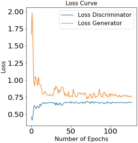
The loss curves for both the $\mathcal{D}$ and $\mathcal{G}$ are shown in Figure 2. This plot shows the change in loss with respect to the number of epochs for the $\mathcal{D}$ and $\mathcal{G}$ architectures described in Section 3.2. The loss curves for both networks appear stable at 150 training epochs while still exhibiting small fluctuations as expected in the training.

Figure 2. Loss curves for the $\mathcal{D}$ and $\mathcal{G}$ of the CGAN. The values indicate the $\mathcal{D}$’s classification on both real and generated data for the July data set. Note, the Keras package in python was used for the training process and calculation of the binary cross entropy loss. This package uses $\mathit{lo}{g}_e$ instead of $\mathit{lo}{g}_2$.

The $\mathcal{D}$’s classification performance on the real and generated data can be examined by interpreting the confusion matrix of the final classifications made by the $\mathcal{D}$ (Table 1). This table shows that the true negatives are higher than the false positives which implies that the $\mathcal{D}$ can detect the generated data more easily then it can detect the real data. Both the true positives and false negatives are more evenly split, implying that the $\mathcal{D}$ has more difficulty classifying the real data as real.

Table 1. Confusion matrix outputs for the CGAN using the July data set.

Metric	Metric Interpretation	Value
True Positives	classifies real as real	1406
True Negatives	classifies generated as generated	2170
False Positives	classifies generated as real	912
False Negatives	classifies real as generated	1676

Metrics: Column Shapes, Correlations, Boundary Adherence, and Synthesis for the July Data Set

To assess the generated data the SDMetrics package in python (SDMetrics 2024e) was used to evaluate the column shapes, correlations, boundary adherence, and synthesis of the data with respect to the real data distribution.

Column Shapes

The column shape of each feature in the generated data set is analyzed using the Kolmogorov-Smirnov (KS) statistic. This statistic converts each numerical distribution into its cumulative distribution function. From here, the maximum difference between the two cumulative distribution functions is determined (SDMetrics 2024c). This metric inverts the statistic and returns $1-\mathit{KS}\mathit{statistic}$.⁹ Therefore, the higher the score the more similar the real and generated data are to one another.

Table 2 reports the column shape metrics of each feature for both vessel types along with the overall average. This table shows that all features report moderate to high column shape values that are $>$0.70. The overall average of the column shapes for each vessel type are high with values $\ge$ 0.86.

Table 2. Column Shape Scores for the generated pleasure craft and cargo vessel data using the July data set.

Feature	Cargo Vessels	Pleasure Craft Vessels
avg_sog	0.95	0.90
start_lat	0.88	0.84
end_lat	0.80	0.85
start_lon	0.72	0.94
end_lon	0.94	0.83
Overall Average	0.86	0.87

Figures 3 and 4 help illustrate what the column shape metric is reporting. To visually compare the real and generated data, scatter plots of the features and the individual feature distributions are presented in these figures. The data sets are color coded where orange represents the real data and blue the generated data. The plots along the diagonal of the figures are the data distributions for each individual feature highlighting the similarities and differences between the real and generated distributions. The distribution plots of the generated data features model the real data features well, as confirmed by the moderate to high column shape values ($>0.70$).

Figure 3. Feature plots and distributions for the pleasure craft vessel type using the July data set. The axes are based on the standardized values for the corresponding feature.

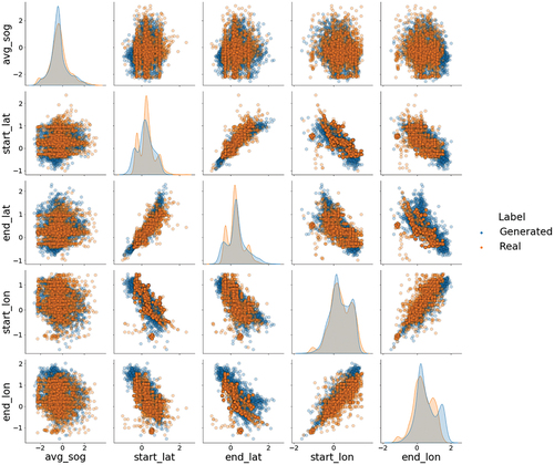
Figure 4. Feature plots and distributions for cargo vessel type using the July data set. The axes are based on the standardized values for the corresponding feature.

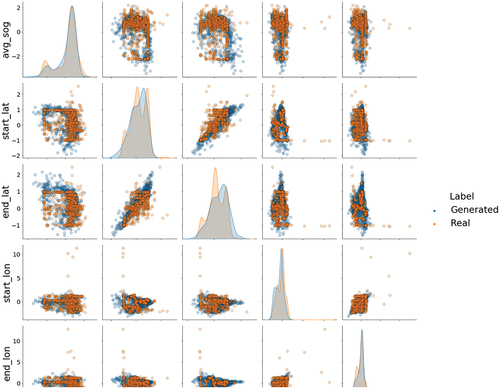
Figures 3 and 4 show that the real data features are multimodal in nature. It is clear that the generated data distributions learned by the $\mathcal{G}$ do not model the different modes perfectly, but do capture the larger scale shapes of the real distributions. The $\mathcal{G}$ seems to struggle with modeling the features that have more distinct modes closer together (e.g., start_lat and end_lat). However, the $\mathcal{G}$ appears to better model multimodal features with two modes when one of the modes does not have a distinct maximum (e.g., start_lon and avg_sog). Nevertheless, the individual modes may be better modeled by developing a network with deeper layers and more nodes that can capture the more complex distributions.

The scatter plots were included as a way to illustrate the density of the data from a different perspective and provide insight to the feature distribution plots. The real data distributions for both vessel types still exhibit a skewness after applying the power transform. It is likely that the cargo vessel type column shape results for the latitudes and longitudes were adversely impacted by the generator’s inability to generate data that mimicked the long right tails seen in the real data distributions. When the scatter plot is taken into consideration for these features, it shows that there are very few points that fall far outside of the distribution. As a result, these points could be considered as outliers that are affecting the overall fit of the distribution.

It is important to note that a design choice of this study was to use a simple architecture for the $\mathcal{G}$ and $\mathcal{D}$ as the data set contained a small set of features. Given the results of the column shape scores shown in Table 2 and the feature distributions in Figures 3 and 4, it is possible that using a deeper and more complex architecture may better capture the nuances within the distributions.

Pairwise Correlations

Column pair trends measure the correlation between the real and generated data for each pairwise feature and calculates the overall average (SDMetrics 2024b). The output ranges from 0 to 1, where a higher value represents a higher similarity between the real and generated data. The column pair trends for the vessel types using the July data set were

• cargo vessels: 0.93

• pleasure craft vessels: 0.94

The column pair trends for both vessel types are high as both are $>$0.90. This shows that generated and real data features within the data set for both vessel types are similar.

Figures 5 and 6 show two visualizations in a single figure. The left side of the figures show the correlation plot of the features from the real data set while the right sides show the correlation plot of the features from the generated data. Comparing the correlation plots of the real and generated data for a specific vessel type can show how similar the correlation relationships are between both data sets.

Figure 5. Correlation plots for real data (left) and generated data (right) for the cargo vessel type using the July data set. The scale indicates the strength of the relationship between the two features, where 1 is perfectly correlated.

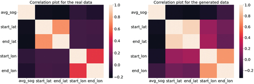
Figure 6. Correlation plots for real data (left) and generated data (right) for the pleasure craft vessel type using the July data set. The scale indicates the strength of the relationship between the two features, where 1 is perfectly correlated.

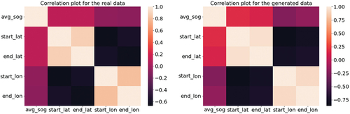
The correlation plots of the real and generated data appear visually similar for both vessel types. This implies that the correlations between the features in the generated data closely mimic that of the real data. However, it is noted that for the cargo vessel type the real and generated correlation plots have greater visual intensity variations as compared to the pleasure crafts, showing that the correlations for the cargo vessel type are not modeled as well as the pleasure crafts. Such comparisons are important when training certain types of ML models as they use the relationships within the feature space to make predictions and classifications. This is important when training certain types of ML models as they use the relationships within the feature space to make predictions and classifications.

Boundary Adherence

Boundary adherence measures whether the generated data for each feature respects the minimum and maximum values of the real data (SDMetrics 2024a). The boundary metric returns the percentage of generated rows that fall within the real data boundaries. The average feature boundary adherence’s for the July data set were as follows:

• Cargo Vessels: 0.98

• Pleasure Crafts: 0.99.

This shows that the generated data respects the boundaries of the real data.

Synthesis

New row synthesis reports the number of new rows generated and if there were any copies of the real data (SDMetrics 2024d). For the generated July data set, both vessel types reported that all of the synthetic data points were new and there were no copies of the real data.

Machine Learning Efficacy Evaluation

Machine learning efficacy is a common approach used to evaluate the performance of synthetic data (Brenninkmeijer 2019). There are a number of ways to perform an efficacy test. The methods differ in how the training and testing data sets are selected. For this study, the machine learning efficacy test was conducted by training classification models on the generated data and then testing each model on real data. The models are trained to classify the data by vessel type: pleasure crafts and cargo ships. The three machine learning methods used were decision tree, random forest, and multi-layer perceptron (MLP). The result of this efficacy test shows how well the method can classify vessel types from the real data based on the model that was developed using the generated data from the CGAN.

As a baseline, the models were first trained and tested on the real data in order to see how well this classification task can be performed. The results for the July data set are shown in Table 3 and the calculated F1 scores¹⁰ are used to measure the success of the model. All three classification models performed with F1 scores $\ge 0.84$ with an overall performance average of 0.89. The overall average of the F1 scores for the individual vessel types were 0.83 and 0.89 for cargo ships and pleasure crafts, respectively. These results show that the classification models had more success at classifying pleasure crafts then cargo ships.

Table 3. Results from machine learning efficacy test using real data for training and testing. This test was performed using the July data set.

ML Technique	F1 Score	F1 Cargo	F1 Pleasure Craft
Decision Tree^a	0.87	0.81	0.93^a b c
Random Forest^b	0.95	0.93	0.97
Multi-layer Perceptron^c	0.84	0.76	0.93
Overall Average	0.89	0.83	0.94

^aThe decision tree model set: max depth = 7.

^bThe random forest model set: the number of estimators = 20.

^cThe multi-layer perceptron set: first layer = 8 nodes, second layer = 10 nodes, third layer = 8 nodes, activation function = relu, optimizer = adam, and iterations = 800.

Table 4 displays the classification test performance using the generated data for the training process and the real data points for the testing of the models. It is important to note that the classification model architectures for the results in Tables 3 and 4 are identical. All models trained using the generated data were able to classify the real data with a F1 score $\ge$ 0.77 with an overall average of 0.80.

Table 4. Results from machine learning efficacy test using generated data to train the model and real data for testing. This test was performed using the July data set.

ML Technique	F1 Score	F1 Cargo	F1 Pleasure Craft
Decision Tree^a	0.80	0.70	0.88
Random Forest^b	0.80	0.72	0.88
Multi-layer Perceptron^c	0.77	0.70	0.85
Overall Average	0.80	0.71	0.87

^aThe decision tree model set: max depth = 7.

^bThe random forest model set: the number of estimators = 20.

^cThe multi-layer perceptron set: first layer = 8 nodes, second layer = 10 nodes, third layer = 8 nodes, activation function = relu, optimizer = adam, and iterations = 800.

When examining the classification performance of each vessel type for the models trained on the real and generated data the overall averaged F1 scores show a 12% and 7% difference in performance for cargo ships and pleasure crafts, respectively. However, the results from the classification models trained with generated data follow the same pattern of the models trained on real data where the success of classifying the pleasure crafts is higher then for cargo ships.

Overall, the results from this efficacy test show promise toward the use of generated data for model development deployed in a real-world setting for vessel tracking characteristics. In order to improve the classification results of models trained with generated data, a more complex CGAN architecture could be explored to improve the modeling the real data.

Comparison of Real and Generated Displacement Tracks

To visually compare the real and generated data for both vessel types, the starting and ending coordinates were used to create displacement tracks. These displacement tracks are illustrated in Figures 7 and 8, respectively. Note, outlier tracks were removed so a closer view of the generated displacement tracks could be displayed.

Figure 7. Plots illustrating the displacement tracks created by the starting and ending coordinates for the pleasure crafts. The left plot and right plot show the displacement tracks for the real data and generated data, respectively. The star represents the end of the displacement track. These plots represent the displacement tracks generated for the month of July.

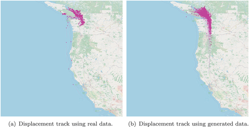
Figure 8. Plots illustrating the displacement tracks created by the starting and ending coordinates for the cargo vessels. The left plot and right plot show the displacement tracks for the real data and generated data, respectively. The star represents the end of the displacement track. These plots represent the displacement tracks generated for the month of July.

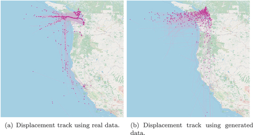
These figures show that the generated displacement tracks are localized to the same regions as the real displacement tracks. However, it is clear that the generated displacement tracks are generalized within the region and not as tightly bound to the traveled paths in the real data. For example, when observing the generated data some of starting and ending positions of the displacement tracks appear on land masses. This is likely a result of the real-world relationship between latitude and longitude being broken in the generated data. The validly of the vessel’s latitude and longitude positions is dictated by it being over water. A possible approach to rectifying this issue is to incorporate a feature into the model that represents the relationship between the latitude and longitude values or incorporate land constraints.

In addition, when examining the location of the start and end points for the real data, it is observed that they tend to be concentrated in similar areas. For example, the end point of a displacement track is represented by the star symbol and these points seem to have a higher concentration of points grouped near the coastline, likely near a location suitable for docking. As a result, the real data displacement tracks follow more consistent route directions as compared to the generated data. The start and end points of the generated displacement tracks are generalized and are not concentrated in specific regions. This is another feature that could be incorporated into the model so that route directions can be captured within the modeled regions.

Overall, such results are promising and the generalization of generated data provided by the CGAN can help train models and make them more robust.

Testing the CGAN Model’s Robustness to Seasonal Changes

In this section, additional experiments are conducted using the CGAN model defined in Section 3.2 to generate data from different months of the year. The months of May and September in 2022 were chosen as they cover the changes from spring-to-summer and summer-to-fall using July to represent the summer period. Testing the CGAN architecture on data sets that vary in season will test robustness of the model. Both data sets are fed into the CGAN to generate data and the results are evaluated using the metrics from Section 4.2 and tested with the vessel classification models reported in Section 4.3. Note, winter months that contain seasonal changes were not used for this study.

Assessing Model’s Generation Performance for May and September Data Sets

Table 5 and 6 highlight the results of the evaluation metrics used to assess the generated data with respect to the real data for May and September, respectively. These results will be compared to the July metrics in order to assess the models robustness to seasonal changes.

Table 5. Average of Feature Column Shapes, Correlations, Boundary Adherence, and Synthesis for May 2022 data.

Metric	Cargo Vessels	Pleasure Craft Vessels
Average of feature column shapes	0.86	0.89
Column pair trends	0.97	0.98
Boundary adherence	0.99	1.00
Synthesis	No Copies	No Copies

Table 6. Average of Feature Column Shapes, Correlations, Boundary Adherence, and Synthesis for September 2022 data.

Metric	Cargo Vessels	Pleasure Craft Vessels
Average of feature column shapes	0.86	0.90
Column pair trends	0.95	0.97
Boundary adherence	0.98	1.00
Synthesis	No Copies	No Copies

Column Shapes

The overall average of the column shapes metric for the May and September data sets are consistent with, or better then the July column shape results. For the month of May, the feature distributions of the generated data model the real data well with an overall average column shape value of 0.86 and 0.89 for cargo vessels and pleasure crafts, respectively. For September, the overall column shape value for the cargo vessels is 0.86, where pleasure crafts reported a value of 0.90. Both experiments generate data distributions for cargo ships that are consistent (identical) to the July results based on the column shape averages. However, the results show slight improvements in modeling the pleasure craft feature distributions with an increase in the column shape average of 2% for May and 3% for September.

Figures 9 and 10 illustrate the column shape metric for the May results while Figures 11 and 12 show the results for September. Based on a visual inspection, the generated data distributions model the real distributions well by capturing the larger scale shapes of the real data for both May and September. However, when comparing these distributions to the July results, the CGAN appears to better capture the nuances related to distinct modes (e.g., start_lat and end_lat) in the May and September feature distributions (e.g., start_lat and end_lat). This is evident when examining the pleasure craft feature distributions.

Figure 9. Feature plots and distributions for the pleasure craft vessel type for May 2022. The axes are based on the standardized values for the corresponding feature.

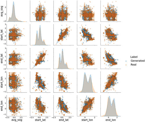
Figure 10. Feature plots and distributions for cargo vessel type for May 2022. The axes are based on the standardized values for the corresponding feature.

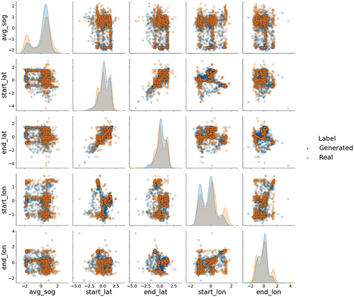
Figure 11. Feature plots and distributions for the pleasure craft vessel type for September 2022. The axes are based on the standardized values for the corresponding feature.

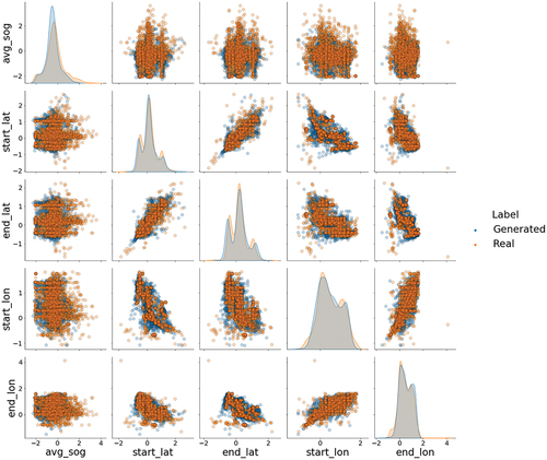
Figure 12. Feature plots and distributions for cargo vessel type for September 2022. The axes are based on the standardized values for the corresponding feature.

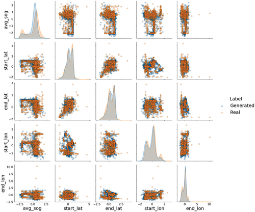
The CGANs ability to model the column shapes (or feature distributions) is unaffected by the changes in season that occur in May and September. However, it is important to note that the distributions of the features for the real data for all three months appear to have similar characteristics. This suggests that the model is robust to the vessel displacement track generation through the spring, summer, and fall months.

Column Pair Trends

The overall column pair trends for the data generated using the May and September data sets are higher than the July results. For May, the column pair trends for both vessel types are 4% higher than the July data, while the September results are 2% and 3% higher for cargo ships and pleasure crafts, respectively. This shows that CGAN model is able to successfully capture and preserve the relationship amongst the features for months that contain seasonal changes.

Boundary Adherence

The overall boundary adherence metric for pleasure crafts and cargo vessels in the month of May and September are consistent with, or better then the July results. Therefore, the boundary adherence is unaffected when using the CGAN model to generate data for the additional months.

Synthesis

The synthesis analysis shows that the generated data sets for both May and September performed similarly to the July data as they did not contain duplicate values. All generated instances were unique.

Machine Learning Efficacy Evaluation

Tables 7 and 8 summarize the results of the efficacy tests performed for May and September, respectively. All models were trained on the generated data and tested on the real data. The results show that efficacy tests are able to classify the real data with an overall averaged F1 score of 0.80 for May and 0.83 for September. These results are consistent with July’s overall F1 score of 0.80.

Table 7. Results from machine learning efficacy test using generated data to train the model and real data for testing for May 2022.

ML Technique	F1 Score	F1 Cargo	F1 Pleasure Craft
Decision Tree^a	0.76	0.71	0.82
Random Forest^b	0.80	0.76	0.85
Multi-layer Perceptron^c	0.82	0.78	0.86
Overall Average	0.80	0.75	0.84

^aThe decision tree model set: max depth = 7.

^bThe random forest model set: the number of estimators = 20.

^cThe multi-layer perceptron set: first layer = 8 nodes, second layer = 10 nodes, third layer = 8 nodes, activation function = relu, optimizer = adam, and iterations = 800.

Table 8. Results from machine learning efficacy test using generated data to train the model and real data for testing for September 2022.

ML Technique	F1 Score	F1 Cargo	F1 Pleasure Craft
Decision Tree^a	0.81	0.75	0.87
Random Forest^b	0.85	0.80	0.90
Multi-layer Perceptron^c	0.82	0.76	0.88
Overall Average	0.83	0.77	0.88

^aThe decision tree model set: max depth = 7.

^bThe random forest model set: the number of estimators = 20.

^cThe multi-layer perceptron set: first layer = 8 nodes, second layer = 10 nodes, third layer = 8 nodes, activation function = relu, optimizer = adam, and iterations = 800.

When comparing the overall averaged F1 score classification results for the different vessel types, the models trained on the data generated from May and September showed consistent results with July classification models. The results for May showed a 4% increase in the classification of cargo ships, while pleasure crafts had a 1% decrease. The results for September showed a 6% increase in classification for cargo ships, while pleasure crafts had a 1% increase. A commonality amongst the efficacy tests performed for each of the three months is the higher classification performance for pleasure craft. This result could be related to the fact that in each of the months there was more data for pleasure crafts then cargo ships.

Nevertheless, these tests show that the CGAN presented in this paper can generate data for different months of the year that include seasonal differences and that is usable for training vessel classification models deployed on real world data.

Discussion

This work shows that the CGAN model presented in Section 3.2 is able to generate synthetic vessel displacement track characteristics that represent the real data for different months of the year, including times where seasonal changes are present.

The CGAN architecture was developed solely on vessel data from July 2022. However, the efficacy tests show that the CGAN generated data was usable for training classification models deployed on real world data for May, July, and September with similar performance outcomes. When comparing the feature distributions of the real data for all three months it was noted that the distributions were similar in shape. This indicates that the overall behavior of the vessel classes amongst these months is similar in nature. Therefore, the CGAN model is robust to the seasonal changes that occur in the different months of the year and does not affect how the model generates the synthetic data.

A curious result in the comparison of real and generated data for the two vessel types is the better model performance for pleasure craft as compared to cargo vessels for all three months as seen in Tables 2 to 8. There are plausible potential reasons for this result.

The presence of data imbalances amongst the different vessel types in each of the data sets. All three datasets had more records and vessels for pleasure craft class than cargo ship. With more data it is possible the CGAN is better able to model the features used to create the vessel displacement tracks.

In addition, pleasure crafts typically occupy a more confined geospatial area. This would in turn mean less scatter in the positional data represented here in the start/end latitudes and longitudes. This geospatial confining is also likely to impact the speed profiles of the pleasure craft, perhaps even restricting the speeds due to pleasure craft density or speed restrictions in the area of pleasure craft operation.

It is then reasonable to think such restrictions could result in the pleasure craft feature profiles for position and speed being more normalized in shape. This would in turn provide a better feature environment for the CGANs and quite likely produce better overall results.

The restrictions are visible in the data. For pleasure craft (Figure 7 left panel), there is considerable variation in latitude with less pronounced variability in longitude. We believe these characteristics manifest themselves as a 3-mode shape for latitude in the feature space (see Figure 3), with longitude appearing to have a smoother tail region to the feature space distribution.

In the case of the cargo vessels, the latitudinal variation could be expected to be smoother as there is a greater volume of cargo vessel traffic visible along the eastern Pacific US coast (Figure 8 left panel). As for longitude, the cargo vessels are confined by a desire to be close to the continent which is oriented north-south from Vancouver Island to the western most region of continental US. There is an exception, this being the tracks near the Baja Peninsula. We believe these tracks are visible as outliers in the feature space and are indicated by the few scattered points in start_lon and end_lon in Figures 4, 10 , and 12.

Exploring the potential relationships between the generated data and the feature space, allows us to better understand what constitutes a well-defined feature space. This will be important when constructing vessel tracks over broad spatial regions where the statistical properties of the feature space may be naturally changing due to constraints or geography.

Conclusion and Future Work

This research explores the generation of displacement tracks using a CGAN model in a constraint-free environment for different months of the year. This work is the first building block toward the goal of generating vessel tracks with constraints. The outcome of the developed model has shown promising results toward this goal as the column shapes, correlation comparisons, and machine learning efficacy test indicates that the generated data is similar to the real data for both cargo vessels and pleasure crafts. The development of this research will help train future ML models involving vessel tracks in ocean areas with various constraints, such as the Arctic.

The future work and next steps in this research include incorporating the temporal component into the data set and model to generate complete vessel tracks. This will follow an analysis of these models when constraints are introduced into the generation process, such as land restrictions, ice, and route constraints that vessels encounter in the maritime environment. New generative model architectures and techniques will be explored to facilitate this research.

Abbreviations

Artificial Intelligence	=	AI
Automatic Identification System	=	AIS
Course Over Ground	=	COG
Conditional Adversarial Network	=	CGAN
Discriminator	=	$\mathcal{D}$
Generative Adversarial Network	=	GAN
Generator	=	$\mathcal{G}$
Kolmogorov-Smirnov	=	KS
Machine Learning	=	ML
Multi-Layer Perceptron	=	MLP
Maritime Mobile Service Identity	=	MMSI
Rectified Linear Unit	=	ReLU
Speed Over Ground	=	SOG

Data Availability Statement

The AIS data set from 2022 used in this experiment is openly available at https://coast.noaa.gov/htdata/CMSP/AISDataHandler/2022/index.html. It was acquired from the National Oceanic and Atmospheric Administration (NOAA) Vessel Traffic Data repository https://marinecadastre.gov/AIS/.

Disclosure Statement

No potential conflict of interest was reported by the author(s).

Supplementary Material

Supplemental data for this article can be accessed online at https://doi.org/10.1080/08839514.2024.2360283

Notes

1. Annotations are labels that assign an instance to a category or group.

2. AIS data provides details about vessel motion including speed, location coordinates, course, etc.

3. The AIS provides both dynamic and static information with respect to vessels. This includes information related to: time, date, speed, course, heading, ship type, ship dimensions, etc.

4. Web site: https://marinecadastre.gov/AIS/data

5. Skew refers to the distortion of symmetrical distribution within the data.

6. Adaptive Moment Estimation is the algorithm used to help determine the optimal network parameters.

7. The batch size is a number of instances that are processed before updating the weights.

8. An epoch is a full pass through the entire training set.

9. This statistic has a range of 0 to 1.

10. The F1 score is the harmonic mean of the precision and recall. The desired value is one which indicates perfect precision and recall.

References

- Arjovsky, M., S. Chintala, and L. Bottou. 2017. Wasserstein generative adversarial networks. In Proceedings of the 34th International Conference on Machine Learning, Sydney, NSW, Australia, PMLR.
- Bao, J., D. Chen, F. Wen, H. Li, and G. Hua. 2017. CVAE-Gan: Fine-grained image generation through asymmetric training. In 2017 IEEE International Conference on Computer Vision (ICCV), October. doi:10.1109/iccv.2017.299.
- Brenninkmeijer, B. 2019. On the generation and evaluation of tabular data using GANs. thesis, Master Thesis Data Science.
- Campbell, J. 2021. Machine learning literacy and applications in defence and security. Defence research and development Canada - scientific report. November.
- Campbell, J., M. Ferreira, and A. Isenor. 2023. Developing generative adversarial networks (GANs) for the generation of synthetic vessel movement data. Defence research and development Canada - scientific report. December.
- Campbell, J. N. A., A. W. Isenor, and M. Dais Ferreira. 2022. Detection of invalid AIS messages using machine learning techniques. Procedia Computer Science 205:229–29. doi:10.1016/j.procs.2022.09.024.
- Chen, L., S. Dai, C. Tao, D. Shen, Z. Gan, H. Zhang, Y. Zhang, and L. Carin. 2020. Adversarial text generation via feature-mover’s distance. arXiv.org August 12, 2020. https://arxiv.org/abs/1809.06297.
- Chen, X., Y. Duan, R. Houthooft, J. Schulman, I. Sutskever, and P. Abbeel. 2016. InfoGAN: Interpretable representation learning by information maximizing generative adversarial nets. In Advances in neural information processing systems, ed. D. D. Lee, U. von Luxburg, R. Garnett, M. Sugiyama, and I. Guyon, 2180–2188. Red Hook, NY, USA: Curran Associates, Inc.
- Esteban, C., S. L. Hyland, and G. Rätsch. 2017. Real-valued (Medical) time series generation with recurrent conditional GANs. ArXiv abs/1706.02633.
- Gao, M., and G.-Y. Shi. 2020. Ship collision avoidance anthropomorphic decision-making for structured learning based on AIS with SEQ-CGAN. Ocean Engineering 217 (December):107922. doi:10.1016/j.oceaneng.2020.107922.
- Goodfellow, I., J. Pouget-Abadie, M. Mirza, B. Xu, D. Warde-Farley, S. Ozair, A. Courville, and Y. Bengio. 2014. Generative Adversarial Nets. Advances in Neural Information Processing Systems 27 63:139–144.
- Gupta, A., J. Johnson, L. Fei-Fei, S. Savarese, and A. Alahi. 2018. Social GAN: Socially acceptable trajectories with generative adversarial networks. In 2018 IEEE/CVF Conference on Computer Vision and Pattern Recognition, Salt Lake City, UT, USA, 2255–64.
- Hazra, T., and K. Anjaria. 2022. Applications of game theory in deep learning: A survey. Multimedia Tools and Applications 81 (6):8963–94. doi:10.1007/s11042-022-12153-2.
- Jin, G., Q. Wang, X. Zhao, Y. Feng, Q. Cheng, and J. Huang. 2019. Crime-Gan: A context-based sequence generative network for crime forecasting with adversarial loss. In 2019 IEEE International Conference on Big Data (Big Data), December. doi:10.1109/bigdata47090.2019.9006388.
- Kosaraju, V., A. Sadeghian, R. Martín-Martín, S. H. R. Ian Reid, and S. Savarese. 2019. Social-Bigat: Multimodal trajectory forecasting using bicycle-gan and graph attention networks. arXiv.org July 17, 2019. https://arxiv.org/abs/1907.03395.
- Liang, K., S. Zhou, M. Liu, Y. Liu, W. Tu, Y. Zhang, L. Fang, Z. Liu, and X. Liu. 2024. Hawkes-enhanced spatial-temporal hypergraph contrastive learning based on criminal correlations. Proceedings of the AAAI Conference on Artificial Intelligence 38 (8):8733–41. doi:10.1609/aaai.v38i8.28719.
- Liao, W., K. Hu, M. Ying Yang, and B. Rosenhahn. 2022. Text to Image Generation with Semantic-Spatial Aware Gan. In 2022 IEEE/CVF Conference on Computer Vision and Pattern Recognition (CVPR), June. doi:10.1109/cvpr52688.2022.01765.
- Li, X., K. Mao, F. Lin, and Z. Feng. 2023. Feature-aware conditional gan for category text generation. arXiv.org. Accessed August 2, 2023. https://arxiv.org/abs/2308.00939.
- Liu, S., H. Liu, H. Bi, and T. Mao. 2020. CoL-GAN: Plausible and collision-less trajectory prediction by attention-based GAN. IEEE Access 8:101662–71. doi:10.1109/ACCESS.2020.2987072
- Liu, Y., R. Yu, S. Zheng, E. Zhan, and Y. Yue. 2019. NAOMI: Non-autoregressive multiresolution sequence imputation. In Guide Proceedings. Accessed December 1, 2019. https://dl.acm.org/doi/10.5555/3454287.3455295.
- Lu, X., M. He, J. Ma, H. Wang, and Y. Shao. 2023. Vessel Trajectory Prediction with the Introduction of Channel Information. In 2023 7th International Conference on Transportation Information and Safety (ICTIS). Accessed August 4, 2023. doi:10.1109/ictis60134.2023.10243977.
- MarineCadastre.gov. 2024. “Vessel Traffic Data.” MarineCadastre.Gov | Vessel Traffic Data. Accessed February 29, 2024. https://marinecadastre.gov/AIS/.
- McArthur, B. A., and A. W. Isenor. 2021. Applying spatial mutual information to AIS DATA. The Journal of Navigation.” Cambridge Core 75 (1):95–105. Accessed October 1, 2021. doi:10.1017/s0373463321000734.
- Mirza, M., and S. Osindero. 2014. Conditional Generative Adversarial Nets.” arXiv.org, Accessed November 6, 2014. https://arxiv.org/abs/1411.1784.
- Mogren, O. 2016. C-RNN-Gan: Continuous recurrent neural networks with adversarial training.” arXiv.org, Accessed November 29, 2016. https://arxiv.org/abs/1611.09904.
- Nan, G., H. Xue, W. Shao, S. Zhao, K. Kai Qin, A. Prabowo, M. Saiedur Rahaman, and F. D. Salim. 2022. Generative adversarial networks for spatio-temporal data: A Survey. ACM Transactions on Intelligent Systems and Technology 13 (2):1–25, February 6. doi:10.1145/3474838.
- Nielsen, M. A. 2015. Neural networks and deep learning. Determination Press. http://neuralnetworksanddeeplearning.com/.
- NOAA. 2024. AIS data for 2020. NOAA office for coastal management. Accessed February 29, 2024. https://coast.noaa.gov/htdata/CMSP/AISDataHandler/2020/index.html.
- OpenAI. 2024a. Dall‧·E 2. Dall‧e 2. Accessed February 29, 2024a. https://openai.com/dall-e-2.
- OpenAI. 2024b. Introducing Chatgpt. Introducing ChatGPT. Accessed February 29, 2024b. https://openai.com/blog/chatgpt.
- Radford, A., L. Metz, and S. Chintala. 2016. Unsupervised representation learning with deep convolutional generative adversarial networks.” arXiv.org, Accessed January 7, 2016. https://arxiv.org/abs/1511.06434.
- Sadeghian, A., V. Kosaraju, A. Sadeghian, N. Hirose, H. Rezatofighi, and S. Savarese. 2019. SoPhie: An attentive GAN for predicting paths compliant to social and physical constraints. In 2019 IEEE/CVF Conference on Computer Vision and Pattern Recognition (CVPR), Long Beach, CA, USA.
- Saxena, D., and J. Cao. 2021. Generative adversarial networks (Gans). ACM Computing Surveys 54 (3):1–42. doi:10.1145/3446374.
- Scikit-learn developers. 2024. Sklearn.Preprocessing.powertransformer. scikit. Accessed February 29, 2024. https://scikit-learn.org/stable/modules/generated/sklearn.preprocessing.PowerTransformer.html.
- SDMetrics. 2024a. “BoundaryAdherence.” BoundaryAdherence - SDMetrics. Accessed February 29, 2024a. https://docs.sdv.dev/sdmetrics/metrics/metrics-glossary/boundaryadherence.
- SDMetrics. 2024b. “CorrelationSimilarity.” CorrelationSimilarity - SDMetrics. Accessed February 29, 2024b. https://docs.sdv.dev/sdmetrics/metrics/metrics-glossary/correlationsimilarity.
- SDMetrics. 2024c. Kscomplement. KSComplement - SDMetrics. Accessed February 29, 2024c. https://docs.sdv.dev/sdmetrics/metrics/metrics-glossary/kscomplement.
- SDMetrics. 2024d. “NewRowsynthesis.” NewRowSynthesis - SDMetrics. Accessed February 29, 2024d. https://docs.sdv.dev/sdmetrics/metrics/metrics-glossary/newrowsynthesis.
- SDMetrics. 2024e. What’s included? What’s included? - SDMetrics. Accessed February 29, 2024e. https://docs.sdv.dev/sdmetrics/reports/quality-report/whats-included.
- Syms, M. S., A. W. Isenor, B. Chivari, A. DeBaie, A. Hogue, and B. Glessing. 2021. Building a maritime picture in the era of big Data: The development of the geospatial communication Interface+. In 2021 International Conference on Military Communication and Information Systems (ICMCIS). Accessed May 4, 2021. doi:10.1109/icmcis52405.2021.9486392.
- Tao, M., H. Tang, F. Wu, X. Jing, B.-K. Bao, and C. Xu. 2022. DF-Gan: A simple and effective baseline for text-to-image synthesis. In 2022 IEEE/CVF Conference on Computer Vision and Pattern Recognition (CVPR), June. Accessed February 29, 2024. doi:10.1109/cvpr52688.2022.01602.thispersondoesnotexist.com. https://thispersondoesnotexist.com/.
- Yonghong, L., X. Cai, Y. Zhang, J. Xu, and X. Yuan. 2018. Multivariate Time Series Imputation with Generative Adversarial Networks. Neural Information Processing Systems 31:1603–1614.
- Yoon, J., D. Jarrett, and M. van der Schaar. 2019. Time-series Generative Adversarial Networks. Neural Information Processing Systems 32:5508–5518.
- Yu, H., Z. Li, G. Zhang, P. Liu, and J. Wang. 2020. Extracting and predicting taxi hotspots in spatiotemporal dimensions using conditional generative adversarial neural networks. IEEE Transactions on Vehicular Technology 69 (4):3680–92. doi:10.1109/TVT.2020.2978450
- Zhang, B., S. Gu, Z. Bo, J. Bao, D. Chen, B. Guo, Y. Wang, and F. Wen. 2022. StyleSwin: Transformer-Based GAN for High-Resolution Image Generation. In Proceedings of the IEEE/CVF conference on computer vision and pattern recognition, New Orleans, LA, USA.
- Zhang, W., W. Jiang, Q. Liu, and W. Wang. 2023. AIS data repair Model based on generative adversarial network. Reliability Engineering & System Safety 240 (December):109572. doi:10.1016/j.ress.2023.109572