Developing Machine Learning-based Control Charts for Monitoring Different GLM-type Profiles With Different Link Functions

ABSTRACT

In certain situations, the quality of a process is determined by dependent variables in relation to independent variables, often modeled through a regression framework referred to as a profile. The practice of monitoring and preserving this relationship is known as profile monitoring. In this paper, we propose an innovative approach that uses different machine-learning (ML) techniques for constructing control charts and monitoring generalized linear model (GLM) profiles with three different GLM-type response distributions of Binomial, Poisson, and Gamma, and by examining different link functions for each response distribution. Through our simulation study, we undertake a comparative analysis of different training methods. We measure the charts’ performance using the average run length, which signifies the average number of samples taken before observing a data point that exceeds the predefined control limits. The result shows that the selection of ML control charts is contingent on the response distribution and link function, and depends on the shift sizes in the process and the utilized training method. To illustrate the practical application of the proposed ML control charts, we present two real-world cases as examples: a drug–response study and a volcano-eruption study, to demonstrate how each ML chart can be implemented in practice.

Introduction

Statistical quality control (SQC) is the utilization of statistical tools and techniques to control a product or service’s quality and is used across a range of industries. It can be divided into three main categories: statistical process control (SPC), design of experiments (DOE), and acceptance samplings.

SPC is a quality control method used to monitor and control a process to ensure that it operates within a specified range of variation. The goal of SPC is to detect and correct process variations before they result in defective products or services. By monitoring and controlling processes, organizations can improve quality, reduce waste, and increase efficiency. More details about SQC can be found in Montgomery (2012).

The main tool in SPC is a control chart. In 1924, the first control chart was introduced by Dr. Walter A. Shewhart. At the same time, the concept of statistical process monitoring started developing.

A special case of SPC is profile monitoring, in which we monitor a relationship over time instead of monitoring quality characteristics. Profile monitoring is used to detect changes or shifts in the relationship between the key variables over time, allowing for proactive action to be taken to address any issues or identify opportunities for improvements. Profile monitoring can be characterized as the relationship between one or more response variables and one or more explanatory variables. This functional relationship is in the form of a regression model. If the regression has one explanatory variable, it is called a simple profile; otherwise, it is called a multiple profile. The focus of this paper is solely on the simple profiles. Profile monitoring using control charts is divided into two phases: Phase I and Phase II. In Phase I, a set of historical data points is available, and the main goal of Phase I is evaluating the process stability and estimating the process parameters from the in-control samples. In most of the studies, as well as in ours, it is assumed that the parameters are estimated before the investigation and the study is performed in Phase II to conduct online monitoring and detect shifts.

Kang and Albin (2000) introduced simple linear profiles with two main applications in semiconductor and food manufacturing. They used the memory-less Hotelling´s T² and memory-type exponentially weighted moving average (EWMA) control charts. A significant development in monitoring simple linear profiles was made by Kim, Mahmoud, and Woodall (2003). Other notable work has been proposed by Zou, Zhang, and Wang (2006). They used a control chart based on a change-point model to monitor linear profiles. More information about different profile types and profile monitoring schemes can be found in Noorossana, Saghaei, and Amiri (2011).

Simple linear profiles are generally used with the assumptions of being quantitative and the normal distribution of the response variable (Amiri et al. 2010; Soleimani, Noorossana, and Amiri 2009). However, these assumptions can be violated in some applications, and instead, generalized linear models (GLMs) can be used to describe the profiles. We can use a range of distributions and different link functions in GLMs. Koosha and Amiri (2011) investigated the effect of link functions on monitoring logistic regression profiles using the Hotelling’s T² control chart. The other types of distributions most commonly used other than the Binomial distribution, are the Gamma and Poisson distributions. Amiri, Koosha, and Azhdari (2012) used the Hotelling’s T²-based methods for monitoring Gamma profiles, while Sharafi, Aminnayeri, and Amiri (2013) used the maximum likelihood estimator approach for estimating the time of the step changes in Poisson regression profiles. Koosha and Amiri (2013) considered a generalized linear mixed model for monitoring autocorrelated logistic regression profiles. Shadman et al. (2014) used a change point approach based on the Rao score test for monitoring GLM profiles. Qi et al. (2016) used the weighted likelihood ratio charts for monitoring GLM profiles. Amiri, Sogandi, and Ayoubi (2018) developed some EWMA-based methods for simultaneous monitoring of the multivariate linear and GLM regression profiles.

One strategy would be using machine learning (ML) techniques for process or profile monitoring for different purposes such as dimension reduction, detection, identification, pattern recognition, and diagnosis. The most common ML techniques used for process monitoring are Support Vector Machines (SVM), Random Forests (RF), and Neural Networks (NN) (Apsemidis, Psarakis, and Moguerza 2020; Escobar and Morales-Mendez 2018; Mohd Amiruddin et al. 2020; Yeganeh et al. 2022; Yeganeh, Pourpanah, and Shadman 2021). In recent years, researchers have combined ML techniques with process monitoring and have used them to construct control charts (Mohammadzadeh, Yeganeh, and Shadman 2021; Sabahno and Amiri 2023; Sabahno and Niaki 2023; Yeganeh et al. 2023; Yeganeh, Chukhrova, et al. 2023; Yeganeh, Johannssen, et al. 2023; Yeganeh, Johannssen, Chukhrova, et al. 2023; Yeganeh et al. 2024). These studies have shown superior performances of the ML-based control charts over the statistics-based control charts.

Sabahno and Amiri (2023) developed statistical and ML control charts for monitoring GLM profiles. However, they only investigated the Binomilly distributed response and the logit link function. In this paper, for the first time in the literature, we investigate different ML techniques, namely SVM, RF, and NN to build control charts for monitoring different GLM profiles with different link functions. To model profiles, we consider three main distributions: Binomial, Gamma, and Poisson, each with three different corresponding link functions detailed in Section GLM Profiles. We simulate data with fixed parameters and try a variety of training methods to obtain the best ML structures to achieve the desired performance. The performances are evaluated regarding the average run length (ARL) with different shift sizes and types. Run length is the number of samples (subgroups) taken before the chart signals a point beyond the control limit. The main purpose of this paper is to use a range of ML techniques to build the control charts and investigate different response distributions and different link functions as well as different training methods for the ML structures to see which one results in better performance (smaller values of ARL).

This paper is structured as follows. In Section GLM Profiles, we introduce the main theory connected with GLM profiles, explain the differences between profiles for different distributions used in this paper, and briefly describe the theory connected with the link functions. Section Machine Learning Techniques follows with a description of ML techniques. Following the introduction of ML techniques, ML control charts are described in Section Control Charts. In Section Simulation Studies, extensive numerical analyses to evaluate the ML control charts with different distributions, link functions, training methods, and shift sizes and types are performed. After the simulation studies, two different illustrative examples are presented in Section Illustrative Examples. Finally, we summarize the results obtained by this study, state our conclusions, and make some suggestions for future research in Section Concluding Remarks.

GLM profiles

We describe GLM profiles according to Sogandi and Amiri (2017) and Olsson (2002). We assume for the kth profile to have a set of n observations $\{(x_{\mathit{j},\mathit{k}},\mathit{\hspace{0.17em}}{y}_{\mathit{j},\mathit{k}}),\mathit{j}=1,\dots ,\mathit{n}\},$ where $x_{\mathit{j},\mathit{k}}$ is a vector of predictor variables and $y_{\mathit{j},\mathit{k}}$ represents the jth response variable in the kth profile. We assume that the relationship between the response $y_{\mathit{j},\mathit{k}}$ and the predictor variables $x_{\mathit{j},\mathit{k}}$ is defined by generalized linear models (GLM), where $x_{\mathit{j},\mathit{k}}$ is a vector of q predictor variables ($x_{\mathit{j},\mathit{k},1},\dots ,x_{\mathit{j},\mathit{k},\mathit{q}})$. As a result, the response variables $y_{\mathit{j},\mathit{k}}$ have the same distribution for each profile. The predictor variables are combined linearly with the coefficients vector ${\beta }_j$ to define the linear predictor ${\mu }_{\mathit{j},\mathit{k}}=x_{j,k}^T{\beta }_j$, where ${\beta }_j=\left({\beta }_{\mathit{j},1},\dots ,{\beta }_{\mathit{j},\mathit{q}}\right)$. We also assume a monotone link function g defined with the following relationship:

$\mathit{g}\left({\eta }_{\mathit{j},\mathit{k}}\right)={\mu }_{\mathit{j},\mathit{k}}=x_{j,k}^T{\beta }_j,$

where ${\eta }_{\mathit{j},\mathit{k}}=\mathit{E}\left(y_{\mathit{j},\mathit{k}}\right)$ and g is a monotone link function. The link functions will be described in the following section. If the value of $x_{\mathit{j},\mathit{k},1}$ is equal to 1, ${\beta }_{\mathit{j},1}$ is the intercept of the model, and in our study we have $\mathit{q}=2$. Most of the studies in profile monitoring assume that the response variable follows the Normal distribution. However, in this paper, we assume that the response variable belongs to the exponential family of distributions and has a Binomial, Poisson, or Gamma distribution, because they are more common in real practices. For the kth profile, the probability distribution belongs to the exponential family if it can be written as:

$\mathit{f}\left(y_{\mathit{j},\mathit{k}},{\theta }_{\mathit{j},\mathit{k}},{\varphi }_{\mathit{j},\mathit{k}}\right)=\exp \left(\frac{\left({\mathit{y}}_{\mathit{j},\mathit{k}}{\theta }_{\mathit{j},\mathit{k}}-\mathit{b}\left({\theta }_{\mathit{j},\mathit{k}}\right)\right)}{\mathit{a}\left(y_{\mathit{j},\mathit{k}}\right)}+\mathit{c}\left(y_{\mathit{j},\mathit{k}},{\theta }_{\mathit{j},\mathit{k}}\right)\right),$

where $\mathit{a}\left(.\right),\mathit{b}\left(.\right)$ and $\mathit{c}\left(.\right)$are some functions, and ${\varphi }_{\mathit{j},\mathit{k}}$ is the dispersion parameter. ${\varphi }_{\mathit{j},\mathit{k}}$ is the canonical parameter representing some function of the location parameter of the distribution. More information about these functions and parameters for the corresponding distribution can be found in Olsson (2002).

Link functions transform the probabilities of the levels of a categorical response variable to a continuous scale that is unbounded. Link function g represents a relationship between the mean of the response variable and the explanatory variables as:

$\mathit{g}\left(\mathit{E}\left(\mathit{Y}\right)\right)=X^T\mathit{\beta }.$

We also know the canonical link functions. The canonical link functions transform the mean to a canonical location parameter of the exponential family member. For the canonical link function $\mathit{g}\left(.\right)$, we have $\mathit{g}\left(\mathit{E}\left(\mathit{Y}\right)\right)=\mathit{\theta }$. So for the Binomial distribution, the canonical link is logit, for the Poisson is log and for the Gamma is negative inverse. There are also some references where the Gamma distribution has different parametrization or the canonical link function (e.g. in Myers et al. 2010, it is mentioned that the canonical link function is inverse). The choice of the link function mostly depends on the data type and there are times when the canonical link may not be appropriate. Therefore, we define the most common link functions in the following tables, which are later used for the corresponding distributions. For the Binomial distribution from Table 1 we have for the cloglog link function${\mu }_B=1-\exp \left(-exp\left(X^T\mathit{\beta }\right)\right)$, for the logit link function ${\mu }_B=\frac{\exp \left(X^T\mathit{\beta }\right)}{1+\exp \left(X^T\mathit{\beta }\right)}$ and for the probit link function ${\mu }_B={\varphi }^{-1}\left(X^T\mathit{\beta }\right)$, where ${\mu }_B$ represents the mean value for the Binomial distribution.

Table 1. Link functions for Binomial distribution.

Type	$\mathit{Link}\mathit{function}{\nu }_B=\mathit{g}\left({\mathit{\mu }}_B\right)$	$\mathit{Inverse}\mathit{link}\mathit{function}{\mathit{\mu }}_B=g^{-1}\left({\nu }_B\right)$
Cloglog	$\ln \left(-ln\left(1-{\mathit{\mu }}_{\mathit{B}}\right)\right)$	$1-\exp \left(-exp\left({\mathit{\nu }}_B\right)\right)$
Logit	$ln\left(\frac{{\mathit{\mu }}_{\mathit{B}}}{1-{\mathit{\mu }}_{\mathit{B}}}\right)$	$\frac{\exp \left({\mathit{\nu }}_B\right)}{1+\exp \left({\mathit{\nu }}_B\right)}$
Probit	${\varphi }^{-1}\left({\mathit{\mu }}_{\mathit{B}}\right)$	$\mathit{\varphi }\left({\mathit{\nu }}_B\right)$

For the Poisson distribution from Table 2 we have the identity link function $\mathit{\lambda }=X^T\mathit{\beta }$, the log link function $\mathit{\lambda }=\exp \left(X^T\mathit{\beta }\right)$, and the sqrt link function $\mathit{\lambda }=(X^T\mathit{\beta }{)}^2$.

Table 2. Link functions for Poisson distribution.

Type	$\mathit{Link}\mathit{function}{\nu }_P=\mathit{g}\left(\mathit{\lambda }\right)$	$\mathit{Inverse}\mathit{link}\mathit{function}\mathit{\lambda }=g^{-1}\left({\nu }_P\right)$
Identity	$\mathit{\lambda }$	${\mathit{\nu }}_P$
Log	$\ln \left(\mathit{\lambda }\right)$	$\exp \left({\mathit{\nu }}_P\right)$
Sqrt	$\sqrt{\mathit{\lambda }}$	${{\mathit{\nu }}_P}^2$

For the Gamma distribution from Table 3 we have the identity link function ${\mu }_G=\mathit{\kappa \omega }=X^T\mathit{\beta }$, the inverse link function ${\mu }_G=\mathit{\kappa \omega }=(X^T\mathit{\beta }{)}^{-1}$, and the log link function ${\mu }_G=\mathit{\kappa \omega }=\exp (X^T\mathit{\beta })$.

Table 3. Link functions for Gamma distribution.

Type	$\mathit{Link}\mathit{function}{\nu }_G=\mathit{g}\left({\mathit{\mu }}_G\right)$	$\mathit{Inverse}\mathit{link}\mathit{function}{\mathit{\mu }}_G=g^{-1}\left({\nu }_G\right)$
Identity	${\mathit{\mu }}_{\mathit{G}}$	${\mathit{\nu }}_G$
Inverse	${{\mathit{\mu }}_{\mathit{G}}}^{-1}$	${{\mathit{\nu }}_G}^{-1}$
Log	$\ln \left({\mathit{\mu }}_{\mathit{G}}\right)$	$\exp \left({\mathit{\nu }}_G\right)$

Machine Learning Techniques

We use several ML techniques to build control charts, namely Support Vector Machine (SVM), Random Forest (RF), and Neural Networks (NN), which are briefly described in what follows.

Support Vector Machine

SVM is one of the supervised learning algorithms used for the analysis of data in classification or regression problems. In the case of a regression problem, it is called SVR. The algorithm was first proposed by Boser, Guyon, and Vapnik (1992). The goal of SVM is to transform the input space to a higher dimensional feature space through a mapping function and to construct a separating hyperplane with maximum distance from the closest points, called support vectors.

The kernel functions are used for the transformation of the input space to a higher dimensional feature space. The most commonly used kernel functions are linear, polynomial, sigmoid, and radial basis. The process of training an SVM involves solving a quadratic optimization problem to find the optimal solution. For optimization, in our case, the computer package uses the sequential minimization optimization algorithm. For more information about SVM, we refer interested readers to Stoean and Stoean (2014).

Random Forest

RF is another ML algorithm that is widely used in classification and regression problems. It is a statistical learning method based on the principle of ensemble learning, which combines an ensemble (group of trained models). An RF algorithm consists of many decision trees. We can also call them the building blocks of the RF. Ensemble learning combines predictions (by taking the average in a regression case or choosing the class with the maximum number of occurrences in a classification case) from multiple ML algorithms to make a more accurate prediction than a single model (a decision tree, in the RF case). There are several ways to improve the model. We can specify the maximum depth of the trees, increase or decrease the number of trees, and specify the maximum number of features to be included at each node split. Increasing the number of trees can increase the precision of the prediction. For more information about RF, readers are referred to Breiman (2001).

Neural Networks

The last ML technique used in this paper is NN, whose name and structure are inspired by the human brain. It can be described as a set of algorithms designed to recognize a pattern in a dataset. A NN consists of an input layer, one or more hidden layers, and an output layer.

We will only consider one hidden layer in this research. NNs with more than one hidden layer are called deep learning techniques. Nodes from one layer to another are connected with weight parameters. The problem of an NN is to determine the optimal values of the connection weights and node biases. Node bias refers to a constant input value added to each node, affecting its activation and allowing the network to account for the varying importance of different nodes. In this paper, we use the Broyden-Fletcher-Goldfarb-Shanno optimization method. The most popular NNs are multilayer perceptron, convolutional, and recurrent NNs. More information about NNs can be found in Patterson (1998).

Control Charts

Control charts are the main tool of the SPC and they check whether the process is stable or not (in-control or out-of-control). The values of a measured characteristic (statistic) must be within control limits, otherwise the process is called out-of-control.

Developing control charts involves Phases I and II. In Phase-I, it is necessary to ensure the stability of the process and estimate the in-control values of the process parameters, whereas in Phase II, we monitor the future observations (online monitoring) to detect any shift in the process from the in-control state determined in Phase-I.

Many quality characteristics can be expressed in terms of numerical measurements. We call single measurable characteristics (such as weight, volume, or dimension) variables. That is one type of statistical control charts. Another type of control charts can be for attribute data (such as counts or percentages). More information about variable and attribute control charts can be found in Montgomery (2012).

In the construction of control charts for process monitoring, we consider sample size, sampling interval, and control limits. Usually, sample size and sampling interval are fixed, and the control limit can be obtained with the following algorithm:

Step 1: Set the values of the probability of Type-I error $\mathit{\alpha }$ and sample size n.

Step 2: Find a suitable statistic based on the problem at hand.

Step 3: Generate and sort 10,000 in-control samples in ascending order using the statistic from Step 2. The initial value of UCL will be the $\left[10000\left(1-\mathit{\alpha }\right)\right]$th value in this set.

Step 4: Run at least 5000 simulations and adjust UCL to obtain $\mathit{ARL}=\frac{1}{\alpha }$.

ML Control Charts

In this paper, we focus on the ML control charts similar to Sabahno and Amiri (2023). We consider three input variables, the estimated slope $\widehat{{\beta }_0}$, intercept $\widehat{{\beta }_1}$, and sample mean $\bar{Y}$ for all the ML control charts. The output variable is a continuous variable that generates a linear number (regression output). As a result, we call the SVM, support vector regression (SVR), and we call the RF, random forest regression (RFR). An out-of-control signal is triggered provided that $\mathit{output}>\mathrm{UCL}$.

UCL is an upper control limit and is obtained using the following algorithm:

Step 1: For each distribution, link function, training method, and regression parameters values, we generate in-control and out-of-control data consisting of the estimated regression intercepts, slopes, and means of the response variables as predictor variables (inputs for the ML structure).

Step 2: Assign 0 to the response variable for the in-control training data and 1 to the response variable for the out-of-control training data.

Step 3: Train the ML structure with the training data in regression form (the training data will be described in Section Simulation Studies).

Step 4: Generate 10 000 samples from the in-control process.

Step 5: Set the value of the probability of Type-I error $\mathit{\alpha }$.

Step 6: Sort ML structure outputs in an ascending order.

Step 7: The initial value of UCL will be the $\left[10000\left(1-\mathit{\alpha }\right)\right]$th value in the set.

Step 8: Run at least 5000 simulations and adjust UCL to obtain $\mathit{ARL}=\frac{1}{\alpha }$.

The performance is evaluated with the shifts in the intercept, slope, and simultaneous shifts with the ML structures described in Section Simulation Studies.

Simulation Studies

In this paper, we consider three different training methods. The first training method consists of 2400 profiles, where 1200 are in-control and 1200 are out-of-control. The out-of-control profiles have three types of shifts, namely shifts in the intercept, shifts in the slope, and simultaneous shifts. All types of shifts consist of 400 out-of-control profiles and the shift sizes are equal to 0.1. The second training method consists of 2700 profiles, 1350 in-control profiles, and 1350 out-of-control profiles. The same as the first method, the out-of-control profiles have three types of shifts. In this case, we have three different shift sizes, namely 0.1, 0.5, and 1. We have 150 out-of-control profiles for each size and type. The third training method consists of 1200 in-control and 1200 out-of-control profiles. For the out-of-control profiles, we consider the same types of shifts, but only two shift sizes 0.1 and 1. In this case, we have 200 out-of-control profiles for each type and size. We adopted the first and third training methods from Sabahno and Amiri (2023), and the other one is then proposed with small, moderate, and large shift sizes.

We evaluate the performance of control charts using the ARL for different profiles with corresponding distribution and link functions for each training method and ML technique. The ARL represents the average run length, the average number of samples (subgroups) taken before the chart signals (point beyond the control limits). In addition, we mention the SDRL (standard deviation of run length) as additional information. Changes are made in the profile parameters and a step change of size $\mathrm{\Delta }={\left({\delta }_1,{\delta }_2\right)}^{\mathit{T}}$ occurs in the profile parameters, where ${\delta }_1$ and ${\delta }_2$ represent changes in the intercept and slope in terms of its standard deviation, so ${\sigma }_1$ and ${\sigma }_2$ are the standard deviations of the intercept and slope parameters adopted from different studies to be mentioned. To calculate the ARL and SDRL, we use the following algorithm:

This algorithm is used for the calculation of UCL in the in-control situation with ${\delta }_1=0$ and ${\delta }_2=0$as described in Section ML Control Charts. Assuming $\mathit{\alpha }$ = 0.005, the ARL value for the in-control situation is set to 200 for all the control charts. We also use the algorithm for evaluation of the performance and calculation of the ARL and SDRL in the out-of-control situations (${\delta }_1$and/or${\delta }_2\ne 0)$.

We use similar shift sizes as used in Mohammadzadeh, Yeganeh, and Shadman (2021). For training models, R packages e1071/svm (Meyer 2023), randomForest (Liaw and Wiener 2022), and nnet (Ripley and Venables 2023) are used, in which there are built-in functions for training the corresponding ML techniques. In the case of the SVR, we use the svm() function with default settings, except for the kernel function type. We consider linear, polynomial, radial, and sigmoid kernels to find the best one for each model by considering the performance and the root mean square error (RMSE). For the RFR, we use the randomForest() function by changing the number of trees, other than that, we use the default setting. The same as before, we try to find the best number of trees according to the performance and the RMSE. We use the nnet() function for training the NN. We use the default setting and only vary the number of nodes for the hidden layer and the number of iterations. To be as consistent as possible, we build the NN model with a small number of nodes. We also consider the RMSE and the performance as in previous cases. The obtained RMSEs and the package settings for all the following simulation studies are not reported in this paper to save space but they are available in table formats and can be requested from the corresponding author.

Binomial Profiles

For the Binomial profiles described in Section GLM Profiles, we assume $y_{\mathit{j},\mathit{k}}\sim \mathit{Bin}\left(\mathit{m},p_{\mathit{j},\mathit{k}}\right)$, where $\mathit{m}=30$ is the number of observations and $p_{\mathit{j},\mathit{k}}$ represents the probability of success in the kth profile for the jth observation. It is defined by the following relationship with the same simulation setting as in Shadman et al. (2014):

$\mathit{g}\left(p_{\mathit{j},\mathit{k}}\right)={\beta }_0+{\beta }_1{x}_{\mathit{j},\mathit{k}},$

where the in-control parameters are set to ${\mathit{\beta }}_0={\left(-2.8,1\right)}^T$. The values of the predictor variable are $0.1,0.2,0.3,0.4,0.5,0.6,0.7,0.8,0.9,1$ with and corresponding link function $\mathit{g}$. The out-of-control setting is defined for the parameters as ${\mathit{\beta }}_{1\mathit{\hspace{0.17em}}}={\mathit{\beta }}_0+\mathrm{\Delta }$, where $\mathrm{\Delta }={\left({\sigma }_1{\delta }_1,{\sigma }_2{\delta }_2\right)}^{\mathit{T}}$. The covariance matrix of the Binomial regression parameters is

$\sum =\left[\begin{array}{cc}{{\sigma }_1}^2& {\sigma }_1{\sigma }_2\\ {\sigma }_1{\sigma }_2& {{\sigma }_2}^2\end{array}\right]=\left[\begin{array}{cc}0.2186& -0.2936\\ -0.2936& 0.4771\end{array}\right].$

Hence, ${\sigma }_1=0.4676$ and ${\sigma }_2=0.6907$.

For the Binomial distribution with the logit link function in Tables 4, 5 and 6, we investigate different shift sizes of the intercept, slope, and simultaneous shifts using the ARL with different training methods and ML control charts. In the case of the first training method, we obtain the smallest values of ARL with the SVR control chart. We see different results for the second training method. The smallest values of ARL are for the NN control chart with some exceptions under shifts in the slope and simultaneous shifts (see Tables 5 and 6). For the third training method, we obtain the smallest values of ARL with the SVR control chart, except for the smallest and largest shift sizes in the intercept, slope, and simultaneous shift. In these cases, we obtain the smallest values of ARL with the NN control chart. We can see that the ARL values decrease with increasing shift sizes for all the control charts except for the RFR control chart with the first training method.

Table 4. ARL (SDRL) values of the SVR, RFR and NN control charts under different shifts in the intercept for Binomial distribution with the logit link function.

δ1	Training method
	First training method			Second training method			Third training method
	Control chart			Control chart			Control chart
	SVR	RFR	NN	SVR	RFR	NN	SVR	RFR	NN
0.1	104.51 (103.47)	156.33 (155.57)	112.36 (111.11)	101.97 (102.51)	104.76 (106.76)	99.50 (97.95)	105.19 (105.14)	104.19 (104.01)	102.66 (103.96)
0.3	28.88 (28.03)	101.42 (102.36)	43.08 (41.62)	30.40 (29.73)	34.39 (32.99)	30.13 (29.47)	30.34 (29.92)	34.15 (33.55)	30.32 (28.94)
0.5	10.66 (10.24)	79.90 (77.67)	20.11 (19.73)	10.91 (10.33)	13.55 (12.91)	10.68 (10.01)	10.90 (9.97)	13.08 (12.40)	11.32 (10.63)
0.8	3.23 (2.70)	75.85 (75.07)	8.60 (8.13)	3.50 (2.96)	4.48 (3.92)	3.37 (2.87)	3.48 (2.96)	4.21 (3.82)	3.55 (2.92)
1	1.90 (1.33)	92.81 (90.77)	6.19 (5.70)	2.09 (1.48)	2.68 (2.15)	1.97 (1.40)	2.04 (1.43)	2.48 (1.93)	2.10 (1.55)
2	1.00 (0.02)	>2000 (>2000)	4.55 (4.11)	1.02 (0.07)	1.45 (0.80)	1.01 (0.08)	1.01 (0.05)	1.06 (0.25)	1.01 (0.05)

The smallest numbers in all rows are bolded.

Table 5. ARL (SDRL) values of the SVR, RFR and NN control charts under different shifts in the slope for Binomial distribution with the logit link function.

δ2	Training method
	First training method			Second training method			Third training method
	Control chart			Control chart			Control chart
	SVR	RFR	NN	SVR	RFR	NN	SVR	RFR	NN
0.1	102.21 (102.44)	152.03 (153.64)	103.13 (101.32)	98.42 (97.49)	100.74 (95.78)	99.04 (99.21)	100.81 (99.75)	111.30 (111.41)	98.99 (97.18)
0.3	29.67 (28.64)	92.76 (92.81)	33.48 (33.23)	28.68 (27.79)	31.86 (31.64)	27.06 (26.37)	28.98 (29.12)	34.64 (34.51)	28.80 (27.73)
0.5	10.40 (9.69)	67.77 (65.54)	12.57 (12.11)	10.14 (9.48)	11.23 (10.69)	9.90 (9.46)	10.14 (9.45)	12.58 (12.24)	10.46 (9.73)
0.8	3.18 (2.66)	54.22 (53.52)	4.53 (3.99)	3.21 (2.71)	3.78 (3.22)	3.03 (2.46)	3.18 (2.64)	4.07 (3.58)	3.30 (2.76)
1	1.84 (1.27)	58.23 (57.48)	2.76 (2.22)	1.91 (1.29)	2.22 (1.63)	1.82 (1.23)	1.87 (1.30)	2.32 (1.71)	1.98 (1.41)
2	1.00 (0.03)	>2000 (>2000)	1.64 (1.03)	1.01 (0.06)	1.07 (0.27)	1.10 (0.32)	1.00 (0.05)	1.12 (0.37)	1.01 (0.04)

The smallest numbers in all rows are bolded.

Table 6. ARL (SDRL) values of the SVR, RFR, and NN control charts under different simultaneous shifts for Binomial distribution with the logit link function.

(δ1,δ2)	Training method
	First training method			Second training method			Third training method
	Control chart			Control chart			Link function
	SVR	RFR	NN	SVR	RFR	NN	SVR	RFR	NN
(0.1,0.1)	50.97 (51.84)	123.98 (120.67)	62.46 (60.11)	51.39 (52.41)	58.65 (58.26)	52.57 (52.58)	51.66 (52.86)	58.42 (57.62)	50.30 (50.39)
(0.3,0.1)	17.09 (16.17)	85.41 (84.46)	26.17 (25.42)	17.54 (17.07)	21.03 (20.16)	17.12 (16.61)	17.53 (16.28)	20.40 (20.32)	17.59 (16.41)
(0.4,0.1)	10.33 (9.65)	77.62 (77.87)	17.55 (16.97)	10.93 (10.27)	13.17 (12.79)	10.61 (10.18)	10.67 (10.06)	13.06 (12.41)	10.97 (10.57)
(0.3,0.4)	4.53 (3.96)	61.07 (59.29)	7.06 (6.44)	4.50 (3.92)	5.76 (5.27)	4.51 (3.94)	4.58 (3.91)	5.92 (5.39)	4.61 (4.13)
(0.9,0.1)	1.90 (1.32)	86.23 (83.91)	5.29 (4.71)	2.05 (1.48)	2.63 (2.04)	1.94 (1.34)	1.97 (1.34)	2.45 (1.90)	2.04 (1.41)
(0.5,0.6)	1.57 (0.92)	77.73 (77.58)	2.82 (2.28)	1.60 (0.97)	1.97 (1.35)	1.57 (0.93)	1.62 (0.98)	1.95 (1.36)	1.66 (1.06)
(0.3,0.9)	1.36 (0.70)	82.77 (82.22)	2.13 (1.59)	1.37 (0.72)	1.61 (1.01)	1.35 (0.68)	1.35 (0.70)	1.61 (1.01)	1.39 (0.75)
(0.8,0.5)	1.22 (0.52)	134.01 (128.70)	2.44 (1.89)	1.24 (0.55)	1.50 (0.87)	1.23 (0.54)	1.24 (0.54)	1.41 (0.75)	1.25 (0.55)
(1,0.6)	1.04 (0.20)	>2000 (>2000)	1.97 (1.39)	1.05 (0.24)	1.20 (0.49)	1.04 (0.22)	1.05 (0.23)	1.14 (0.40)	1.06 (0.24)
(0.8,1)	1.01 (0.09)	>2000 (>2000)	1.49 (0.83)	1.01 (0.10)	1.09 (0.32)	1.01 (0.12)	1.01 (0.10)	1.07 (0.26)	1.01 (0.10)

When we compare the overall results, the first training method generally delivers the smallest values of ARL under shifts in the intercept with the SVR control chart except for the smallest shift size. Under shifts in the slope, we obtain the smallest values of ARL with the SVR and NN control charts and the second training method, depending on the shift sizes (see Table 5). Under simultaneous shifts, we can observe a similar trend to the intercept shifts case. We obtain the smallest values of ARL with the SVR control chart and the first training method with some exceptions (see Table 6).

For the Binomial distribution with the probit link function, using the first training method, the smallest values of ARL are obtained with the SVR control chart. For the other two training methods, the smallest values of ARL are obtained with the NN control chart with some exceptions (see Tables 7, 8 and 9). As mentioned for the logit link function, from a certain value of shift size, the ARL values start to increase as the shift sizes increase, for the RFR control chart and with the first training method.

Table 7. ARL (SDRL) values of the SVR, RFR and NN control charts under different shifts in the intercept for Binomial distribution with the probit link function.

δ1	Training method
	First training method			Second training method			Third training method
	Control chart			Control chart			Control chart
	SVR	RFR	NN	SVR	RFR	NN	SVR	RFR	NN
0.1	90.86 (91.69)	149.65 (151.34)	165.47 (166.97)	90.73 (91.35)	106.33 (105.08)	90.80 (89.55)	122.04 (122.33)	106.72 (105.51)	91.69 (92.18)
0.3	22.37 (22.09)	90.76 (89.99)	117.91 (114.97)	22.53 (22.12)	30.24 (29.72)	21.78 (21.18)	33.29 (32.24)	29.67 (28.85)	23.41 (22.65)
0.5	7.45 (7.06)	73.13 (70.61)	66.38 (64.91)	7.52 (7.13)	10.13 (9.68)	7.19 (6.60)	9.73 (9.23)	9.65 (9.08)	7.45 (7.04)
0.8	2.25 (1.68)	93.69 (92.71)	12.27 (11.87)	2.24 (1.66)	2.90 (2.39)	2.24 (1.67)	2.57 (2.00)	2.74 (2.20)	2.28 (1.72)
1	1.42 (0.78)	183.31 (182.01)	4.30 (3.80)	1.48 (0.86)	1.72 (1.11)	1.41 (0.76)	1.52 (0.88)	1.59 (0.97)	1.44 (0.80)
2	1.00 (0.00)	>2000 (>2000)	1.01 (0.07)	1.89 (1.30)	1.08 (0.30)	1.00 (0.00)	1.10 (0.33)	1.04 (0.20)	1.00 (0.00)

The smallest numbers in all rows are bolded.

Table 8. ARL (SDRL) values of the SVR, RFR and NN control charts under different shifts in the slope for Binomial distribution with the probit link function.

δ2	Training method
	First training method			Second training method			Third training method
	Control chart			Control chart			Control chart
	SVR	RFR	NN	SVR	RFR	NN	SVR	RFR	NN
0.1	84.09 (82.47)	136.71 (135.38)	150.38 (147.11)	85.47 (84.20)	97.48 (99.17)	85.89 (86.22)	111.06 (109.48)	97.36 (96.95)	86.36 (85.65)
0.3	18.30 (17.57)	73.90 (75.44)	86.48 (87.41)	19.23 (18.42)	25.45 (24.60)	19.20 (18.72)	27.42 (27.26)	24.89 (24.51)	18.61 (18.07)
0.5	5.56 (4.93)	61.36 (60.72)	57.53 (55.33)	6.13 (5.54)	8.13 (7.66)	6.05 (5.62)	7.96 (7.43)	7.51 (7.13)	5.77 (5.16)
0.8	1.82 (1.21)	99.45 (99.02)	19.97 (19.23)	1.96 (1.34)	2.43 (1.84)	1.89 (1.30)	2.12 (1.54)	2.19 (1.60)	1.84 (1.26)
1	1.22 (0.52)	>2000 (>2000)	8.31 (7.91)	1.35 (0.71)	1.49 (0.86)	1.28 (0.59)	1.34 (0.68)	1.37 (0.69)	1.24 (0.54)
2	1.00 (0.00)	>2000 (>2000)	1.77 (1.15)	1.57 (0.93)	1.04 (0.20)	1.00 (0.00)	1.06 (0.25)	1.02 (0.15)	1.00 (0.00)

The smallest numbers in all rows are bolded.

Table 9. ARL (SDRL) values of the SVR, RFR and NN control charts under different simultaneous shifts for Binomial distribution with the probit link function.

(δ1,δ2)	Training method
	First training method			Second training method			Third training method
	Control chart			Control chart			Link function
	SVR	RFR	NN	SVR	RFR	NN	SVR	RFR	NN
(0.1,0.1)	40.75 (39.95)	99.06 (99.46)	127.52 (123.86)	41.86 (41.19)	51.75 (51.77)	40.68 (40.12)	60.71 (60.01)	52.09 (53.47)	41.19 (40.54)
(0.3,0.1)	11.80 (11.39)	66.75 (66.81)	87.05 (87.69)	11.96 (11.44)	16.53 (15.99)	11.56 (11.02)	17.34 (16.67)	15.83 (15.19)	12.25 (11.75)
(0.4,0.1)	6.89 (6.39)	60.41 (59.52)	66.49 (66.93)	6.90 (6.30)	9.73 (9.15)	6.95 (6.47)	9.22 (8.67)	9.55 (9.04)	7.14 (6.57)
(0.3,0.4)	2.69 (2.15)	54.07 (54.25)	27.51 (26.65)	2.82 (2.26)	3.68 (3.10)	2.77 (2.19)	3.41 (2.87)	3.43 (2.90)	2.75 (2.21)
(0.9,0.1)	1.40 (0.72)	119.58 (122.57)	4.48 (4.04)	1.44 (0.80)	1.68 (1.06)	1.38 (0.72)	1.53 (0.91)	1.60 (0.97)	1.41 (0.76)
(0.5,0.6)	1.17 (0.45)	191.82 (189.03)	3.87 (3.33)	1.27 (0.61)	1.35 (0.67)	1.18 (0.47)	1.25 (0.55)	1.29 (0.61)	1.18 (0.47)
(0.3,0.9)	1.07 (0.27)	>2000 (>2000)	3.36 (2.75)	1.27 (0.58)	1.19 (0.48)	1.07 (0.28)	1.11 (0.34)	1.13 (0.39)	1.07 (0.28)
(0.8,0.5)	1.04 (0.21)	>2000 (>2000)	1.95 (1.35)	1.30 (0.62)	1.13 (0.39)	1.04 (0.21)	1.07 (0.28)	1.09 (0.31)	1.05 (0.22)
(1,0.6)	1.00 (0.04)	>2000 (>2000)	1.23 (0.52)	2.23 (1.67)	1.04 (0.20)	1.00 (0.04)	1.01 (0.08)	1.02 (0.12)	1.00 (0.04)
(0.8,1)	1.00 (0.00)	>2000 (>2000)	1.20 (0.50)	2.27 (1.76)	1.01 (0.12)	1.00 (0.00)	1.00 (0.04)	1.01 (0.09)	1.00 (0.01)

The smallest numbers in all rows are bolded.

We mostly obtain the smallest values of ARL with the NN control chart and the second training method under shifts in the intercept. Under shifts in the slope, the SVR control chart delivers the smallest values of ARL with the first training method. The results under simultaneous shifts depend on the shifts in the intercept and slope (see Table 9).

The first training method for the Binomial distribution with the cloglog link function delivers the smallest values of ARL with the SVR control chart, except for the shift size 0.1 in the intercept (see Table 10). For the second training method, we obtain the smallest values of ARL with the NN control chart except for some shift sizes in the slope (see Table 11). The results for the third training method are similar to those obtained for the first one. The smallest values of ARL are for the SVR control charts with some exceptions. Here again, we can observe the increasing values of ARL with the RFR control chart by increasing the shift sizes from a certain value (see Tables 10 and 12), using the first training method.

Table 10. ARL (SDRL) values of the SVR, RFR and NN control charts under different shifts in the intercept for Binomial distribution with the cloglog link function.

δ1	Training method
	First training method			Second training method			Third training method
	Control chart			Control chart			Control chart
	SVR	RFR	NN	SVR	RFR	NN	SVR	RFR	NN
0.1	95.77 (96.92)	124.87 (124.86)	94.38 (96.18)	105.42 (104.85)	99.33 (99.80)	93.66 (93.13)	97.51 (95.85)	104.15 (101.97)	98.17 (96.21)
0.3	24.83 (24.09)	58.01 (57.90)	25.55 (24.87)	32.46 (31.93)	28.96 (27.86)	25.28 (24.78)	25.91 (25.30)	31.22 (31.17)	27.62 (27.48)
0.5	8.14 (7.48)	34.07 (33.17)	9.26 (8.63)	11.94 (10.98)	10.53 (10.13)	8.46 (7.92)	8.78 (8.20)	11.90 (11.57)	9.11 (8.61)
0.8	2.48 (1.88)	26.09 (25.23)	3.37 (2.79)	3.72 (3.10)	3.36 (2.81)	2.59 (1.96)	2.74 (2.18)	3.68 (3.08)	2.82 (2.24)
1	1.54 (0.89)	33.61 (33.14)	2.75 (2.17)	2.12 (1.54)	2.01 (1.40)	1.59 (0.96)	1.69 (1.09)	2.19 (1.61)	1.73 (1.11)
2	1.00 (0.01)	>2000 (>2000)	4.10 (3.44)	1.01 (0.05)	1.00 (0.02)	1.00 (0.01)	1.00 (0.02)	1.41 (0.77)	1.01 (0.06)

The smallest numbers in all rows are bolded.

Table 11. ARL (SDRL) values of the SVR, RFR and NN control charts under different shifts in the slope for Binomial distribution with the cloglog link function.

δ2	Training method
	First training method			Second training method			Third training method
	Control chart			Control chart			Control chart
	SVR	RFR	NN	SVR	RFR	NN	SVR	RFR	NN
0.1	92.97 (91.27)	122.42 (121.65)	99.72 (97.25)	91.93 (92.08)	95.27 (95.55)	91.77 (90.29)	92.75 (91.61)	100.70 (97.67)	95.31 (92.07)
0.3	24.76 (24.03)	50.80 (50.16)	33.69 (33.34)	23.53 (22.83)	26.30 (25.33)	22.73 (22.02)	24.38 (23.70)	29.65 (29.71)	24.91 (24.52)
0.5	8.30 (7.87)	27.85 (27.51)	13.03 (12.91)	7.62 (7.14)	9.09 (8.33)	7.77 (7.16)	8.03 (7.71)	10.40 (9.76)	8.12 (7.60)
0.8	2.55 (2.03)	20.06 (19.32)	5.13 (4.58)	2.32 (1.71)	2.79 (2.26)	2.35 (1.76)	2.49 (1.93)	3.02 (2.52)	2.57 (1.97)
1	1.54 (0.91)	26.78 (25.64)	4.14 (3.60)	1.46 (0.80)	1.70 (1.09)	1.48 (0.86)	1.58 (0.95)	1.80 (1.19)	1.55 (0.92)
2	1.00 (0.00)	>2000 (>2000)	3.38 (3.07)	1.00 (0.00)	1.00 (0.00)	1.00 (0.00)	1.00 (0.03)	1.05 (0.23)	1.00 (0.00)

The smallest numbers in all rows are bolded.

Table 12. ARL (SDRL) values of the SVR, RFR and NN control charts under different simultaneous shifts for Binomial distribution with the probit link function.

(δ1,δ2)	Training method
	First training method			Second training method			Third training method
	Control chart			Control chart			Link function
	SVR	RFR	NN	SVR	RFR	NN	SVR	RFR	NN
(0.1,0.1)	46.36 (45.37)	79.32 (78.39)	54.85 (53.99)	49.72 (49.28)	50.83 (51.27)	45.53 (44.67)	46.44 (45.62)	56.70 (55.91)	48.54 (48.47)
(0.3,0.1)	13.81 (13.37)	41.20 (40.97)	15.90 (15.76)	17.30 (16.91)	16.89 (16.42)	13.83 (13.63)	14.40 (13.87)	18.12 (18.03)	15.26 (14.96)
(0.4,0.1)	8.02 (7.55)	32.03 (30.71)	9.98 (9.27)	10.72 (10.19)	10.09 (9.49)	8.43 (7.91)	8.60 (8.15)	11.54 (10.82)	9.04 (8.52)
(0.3,0.4)	3.55 (3.06)	22.19 (22.12)	5.69 (5.25)	3.97 (3.41)	4.24 (3.63)	3.46 (2.89)	3.54 (2.99)	4.80 (4.23)	3.71 (3.21)
(0.9,0.1)	1.56 (0.93)	29.70 (29.07)	2.87 (2.32)	2.04 (1.45)	1.97 (1.40)	1.61 (0.98)	1.65 (1.02)	2.22 (1.69)	1.68 (1.07)
(0.5,0.6)	1.35 (0.67)	32.63 (31.73)	3.48 (2.97)	1.42 (0.78)	1.54 (0.89)	1.33 (0.66)	1.36 (0.68)	1.64 (1.02)	1.35 (0.69)
(0.3,0.9)	1.19 (0.48)	47.53 (47.47)	4.22 (3.62)	1.19 (0.47)	1.29 (0.61)	1.17 (0.44)	1.19 (0.48)	1.36 (0.70)	1.21 (0.49)
(0.8,0.5)	1.10 (0.34)	72.64 (72.57)	4.60 (4.08)	1.18 (0.46)	1.21 (0.50)	1.10 (0.33)	1.11 (0.34)	1.31 (0.64)	1.12 (0.37)
(1,0.6)	1.01 (0.10)	>2000 (>2000)	17.11 (17.04)	1.02 (0.15)	1.03 (0.18)	1.01 (0.10)	1.01 (0.12)	1.11 (0.34)	1.01 (0.11)
(0.8,1)	1.00 (0.02)	>2000 (>2000)	88.51 (86.87)	1.00 (0.06)	1.01 (0.06)	1.00 (0.02)	1.00 (0.05)	1.05 (0.23)	1.00 (0.03)

The smallest numbers in all rows are bolded.

We generally obtain the smallest values of ARL almost for all shift sizes with the SVR control chart and with the first training method under shifts in the intercept. Under shifts in the slope, we obtain the smallest values of ARL with the second training method and the SVR and NN control charts depending on the shift size (see Table 11). Under simultaneous shifts, we obtain the smallest values of ARL with the first training method and the SVR control chart or with the second training method and the NN control chart depending on the shift size (see Table 12).

Poisson Profiles

We use a similar approach for Poisson distribution. We use the same setting as was used in Shadman et al. (2014). The predictor variables are the same as for Binomial profiles and the relationship is defined as:

$\mathit{g}\left({\lambda }_{\mathit{j},\mathit{k}}\right)={\beta }_0+{\beta }_1{x}_{\mathit{j},\mathit{k}},$

with ${\mathit{\beta }}_0={\left(3,2\right)}^T$and also the covariance matrix of the Poisson regression parameters is

$\sum =\left[\begin{array}{cc}{{\sigma }_1}^2& {\sigma }_1{\sigma }_2\\ {\sigma }_1{\sigma }_2& {{\sigma }_2}^2\end{array}\right]=\left[\begin{array}{cc}0.0117& -0.0146\\ -0.0146& 0.0207\end{array}\right].$

Therefore, ${\sigma }_1=0.1082$ and ${\sigma }_2=0.1440$.

First, we will consider Poisson profiles with the log link function. For the first training method, the SVR control chart delivers the smallest values of ARL under shifts in the intercept and simultaneous shifts with some similar performances to the NN control chart (see Tables 13, 14 and 15). Under shifts in the slope, the smallest values of ARL are mostly obtained with the NN control chart (see Table 14). For the second training method, we generally obtain the smallest values of ARL with the NN control chart with some similarities to the performance of the SVR control chart under certain shift types and sizes (see Tables 13, 14 and 15). In the case of the third training method, we obtain the smallest values of ARL with the SVR control chart with some similar performances to the NN control chart.

Table 13. ARL (SDRL) values of the SVR, RFR and NN control charts under different shifts in the intercept for Poisson distribution with the log link function.

δ1	Training method
	First training method			Second training method			Third training method
	Control chart			Control chart			Control chart
	SVR	RFR	NN	SVR	RFR	NN	SVR	RFR	NN
0.1	88.01 (87.65)	153.93 (152.60)	88.06 (87.21)	89.44 (88.84)	97.60 (98.23)	88.03 (86.25)	88.27 (87.56)	94.85 (93.73)	89.48 (88.80)
0.3	21.55 (20.88)	87.97 (86.42)	21.66 (20.97)	22.15 (21.65)	26.07 (25.27)	21.97 (21.54)	22.09 (21.56)	24.93 (24.25)	22.39 (21.84)
0.5	7.29 (6.74)	49.56 (47.17)	7.30 (6.75)	7.41 (6.89)	9.38 (9.02)	7.35 (6.83)	7.36 (6.79)	8.73 (8.42)	7.46 (6.96)
0.8	2.40 (1.78)	29.07 (28.63)	2.41 (1.80)	2.46 (1.85)	3.13 (2.64)	2.46 (1.84)	2.46 (1.87)	2.86 (2.32)	2.47 (1.87)
1	1.55 (0.94)	27.31 (27.10)	1.55 (0.94)	1.58 (0.96)	2.04 (1.42)	1.57 (0.96)	1.58 (0.97)	1.82 (1.22)	1.58 (0.96)
2	1.00 (0.00)	>2000 (>2000)	1.00 (0.00)	1.00 (0.00)	1.30 (0.62)	1.00 (0.00)	1.00 (0.00)	1.07 (0.28)	1.00 (0.00)

The smallest numbers in all rows are bolded.

Table 14. ARL (SDRL) values of the SVR, RFR and NN control charts under different shifts in the slope for Poisson distribution with the log link function.

δ2	Training method
	First training method			Second training method			Third training method
	Control chart			Control chart			Control chart
	SVR	RFR	NN	SVR	RFR	NN	SVR	RFR	NN
0.1	94.29 (94.46)	165.66 (163.51)	94.24 (94.32)	92.78 (92.68)	97.20 (98.84)	88.14 (85.96)	91.55 (91.63)	97.32 (97.66)	92.48 (91.50)
0.3	23.67 (23.19)	88.25 (89.07)	23.73 (23.25)	22.58 (21.94)	26.17 (25.44)	22.49 (21.88)	22.03 (21.55)	26.45 (26.20)	22.15 (21.78)
0.5	7.98 (7.49)	51.10 (50.38)	7.90 (7.42)	7.46 (7.01)	9.59 (9.11)	7.42 (7.02)	7.34 (6.87)	9.33 (8.68)	7.35 (6.80)
0.8	2.68 (2.17)	31.04 (30.64)	2.65 (2.14)	2.52 (1.97)	3.29 (2.66)	2.52 (1.97)	2.50 (1.96)	3.16 (2.60)	2.50 (1.96)
1	1.66 (1.06)	31.62 (32.41)	1.65 (1.05)	1.59 (0.98)	2.08 (1.48)	1.59 (0.98)	1.57 (0.96)	2.00 (1.44)	1.57 (0.96)
2	1.00 (0.04)	>2000 (>2000)	1.00 (0.03)	1.00 (0.03)	1.15 (0.40)	1.00 (0.03)	1.00 (0.03)	1.07 (0.26)	1.00 (0.03)

The smallest numbers in all rows are bolded.

Table 15. ARL (SDRL) values of the SVR, RFR and NN control charts under different simultaneous shifts for Poisson distribution with the log link function.

(δ1,δ2)	Training method
	First training method			Second training method			Third training method
	Control chart			Control chart			Link function
	SVR	RFR	NN	SVR	RFR	NN	SVR	RFR	NN
(0.1,0.1)	44.04 (43.12)	123.29 (126.72)	44.04 (43.36)	43.89 (42.57)	49.60 (48.71)	43.62 (42.42)	43.08 (41.99)	48.70 (48.49)	43.46 (42.38)
(0.3,0.1)	12.29 (11.74)	61.70 (61.49)	12.37 (11.74)	12.36 (11.78)	14.57 (14.42)	12.26 (11.70)	12.29 (11.75)	14.15 (13.76)	12.37 (11.79)
(0.4,0.1)	7.50 (6.83)	49.35 (48.98)	7.52 (6.86)	7.50 (6.93)	9.27 (8.57)	7.47 (6.88)	7.52 (6.93)	8.93 (8.19)	7.59 (7.02)
(0.3,0.4)	3.45 (2.94)	32.57 (32.22)	3.44 (2.94)	3.33 (2.82)	4.35 (3.78)	3.34 (2.83)	3.31 (2.79)	4.09 (3.54)	3.34 (2.83)
(0.9,0.1)	1.54 (0.91)	24.69 (24.22)	1.54 (0.92)	1.56 (0.93)	1.99 (1.37)	1.56 (0.93)	1.57 (0.94)	1.80 (1.20)	1.57 (0.95)
(0.5,0.6)	1.37 (0.72)	28.14 (27.34)	1.37 (0.72)	1.36 (0.71)	1.67 (1.06)	1.36 (0.71)	1.35 (0.70)	1.58 (0.95)	1.36 (0.71)
(0.3,0.9)	1.24 (0.55)	34.82 (35.41)	1.23 (0.54)	1.21 (0.51)	1.51 (0.92)	1.21 (0.51)	1.21 (0.51)	1.40 (0.75)	1.21 (0.51)
(0.8,0.5)	1.13 (0.40)	35.03 (33.95)	1.13 (0.40)	1.12 (0.39)	1.36 (0.71)	1.12 (0.38)	1.12 (0.39)	1.24 (0.57)	1.13 (0.39)
(1,0.6)	1.02 (0.14)	91.68 (93.73)	1.02 (0.14)	1.02 (0.13)	1.18 (0.45)	1.02 (0.13)	1.02 (0.13)	1.07 (0.27)	1.02 (0.13)
(0.8,1)	1.00 (0.06)	>2000 (>2000)	1.00 (0.06)	1.00 (0.06)	1.12 (0.37)	1.00 (0.06)	1.00 (0.05)	1.04 (0.20)	1.00 (0.05)

The smallest numbers in all rows are bolded.

We obtain the smallest values of ARL mostly with the SVR control chart. The smallest values of ARL are with the first training method under shifts in the intercept and with the third training method under shifts in the slope, with some similar performances to the NN control chart (see Tables 10 and 11). Under simultaneous shifts, we obtain the smallest values of ARL with the SVR and NN control charts and with all training methods depending on the shift sizes (see Table 12).

Second, we will consider the sqrt link function for the Poisson profiles. We obtain the smallest values of ARL for the first training method with the SVR control charts (see Tables 16, 17 and 18). For the second and third training methods, we obtain the smallest values of ARL with the NN control chart under shifts in the intercept, and with the SVR control chart under shifts in the slope. However, it is different under simultaneous shifts, in which we obtain the smallest values of ARL with the SVR and NN control charts depending on the shift sizes (see Table 18).

Table 16. ARL (SDRL) values of the SVR, RFR and NN control charts under different shifts in the intercept for Poisson distribution with the sqrt link function.

δ1	Training method
	First training method			Second training method			Third training method
	Control chart			Control chart			Control chart
	SVR	RFR	NN	SVR	RFR	NN	SVR	RFR	NN
0.1	110.68 (111.24)	162.75 (165.70)	131.82 (181.07)	105.48 (104.56)	114.53 (116.53)	104.32 (104.62)	105.80 (103.00)	111.45 (107.67)	105.56 (104.58)
0.3	38.43 (38.84)	101.38 (102.69)	63.86 (63.67)	32.67 (32.62)	38.01 (37.62)	32.08 (31.41)	32.94 (32.93)	39.07 (38.12)	32.67 (32.63)
0.5	15.15 (14.97)	69.95 (66.53)	36.12 (35.63)	12.20 (11.50)	15.70 (15.36)	11.86 (11.33)	12.26 (11.60)	16.02 (15.47)	12.19 (11.51)
0.8	5.27 (4.73)	50.49 (48.41)	20.34 (19.79)	4.10 (3.55)	5.42 (4.95)	3.92 (3.31)	4.15 (3.58)	5.50 (5.09)	4.10 (3.55)
1	3.15 (2.44)	50.72 (52.79)	16.61 (15.50)	2.50 (1.87)	3.20 (2.56)	2.39 (1.78)	2.52 (1.89)	3.22 (2.63)	2.50 (1.86)
2	1.06 (0.24)	>2000 (>2000)	79.81 (79.52)	1.02 (0.14)	1.21 (0.51)	1.02 (0.13)	1.02 (0.15)	1.17 (0.46)	1.02 (0.14)

The smallest numbers in all rows are bolded.

Table 17. ARL (SDRL) values of the SVR, RFR and NN control charts under different shifts in the slope for Poisson distribution with the sqrt link function.

δ2	Training method
	First training method			Second training method			Third training method
	Control chart			Control chart			Control chart
	SVR	RFR	NN	SVR	RFR	NN	SVR	RFR	NN
0.1	159.14 (165.27)	201.12 (198.83)	186.08 (181.07)	165.30 (166.89)	177.25 (177.96)	174.41 (178.25)	163.24 (164.75)	172.47 (172.38)	165.53 (167.04)
0.3	107.52 (107.06)	172.37 (173.12)	147.04 (142.57)	112.12 (112.05)	125.57 (127.54)	120.42 (119.61)	110.37 (110.44)	125.73 (127.55)	112.34 (112.15)
0.5	74.72 (75.99)	150.18 (148.52)	121.35 (118.83)	78.57 (80.81)	91.40 (90.77)	84.40 (82.53)	78.21 (79.92)	92.79 (92.89)	78.86 (81.01)
0.8	43.97 (43.42)	118.91 (118.98)	96.06 (98.11)	45.89 (46.22)	60.82 (59.87)	52.55 (51.67)	45.26 (44.91)	62.74 (62.64)	45.97 (46.32)
1	31.24 (31.20)	104.81 (106.22)	83.95 (83.43)	33.09 (32.86)	44.98 (43.53)	37.88 (36.24)	32.71 (32.58)	47.57 (47.52)	33.13 (32.92)
2	8.05 (7.49)	65.93 (64.63)	46.45 (46.99)	8.50 (7.96)	13.36 (12.77)	10.61 (9.98)	8.41 (7.77)	14.77 (14.42)	8.51 (7.97)

The smallest numbers in all rows are bolded.

Table 18. ARL (SDRL) values of the SVR, RFR and NN control charts under different simultaneous shifts for Poisson distribution with the sqrt link function.

(δ1,δ2)	Training method
	First training method			Second training method			Third training method
	Control chart			Control chart			Link function
	SVR	RFR	NN	SVR	RFR	NN	SVR	RFR	NN
(0.1,0.1)	90.92 (93.32)	151.69 (154.72)	122.17 (121.52)	86.22 (86.14)	95.12 (94.40)	87.40 (88.31)	85.99 (85.69)	97.16 (97.22)	86.38 (86.16)
(0.3,0.1)	32.04 (31.25)	85.85 (87.16)	59.32 (59.66)	27.63 (27.11)	33.47 (32.82)	27.06 (26.32)	27.80 (27.37)	36.14 (36.09)	27.67 (27.15)
(0.4,0.1)	20.42 (19.76)	66.44 (66.59)	43.21 (44.21)	16.70 (15.78)	21.27 (20.90)	16.17 (15.44)	16.94 (16.05)	21.77 (21.42)	16.76 (15.92)
(0.3,0.4)	20.58 (19.82)	68.30 (67.19)	47.68 (47.05)	17.80 (17.26)	22.96 (22.86)	18.34 (17.51)	17.90 (17.38)	23.69 (23.47)	17.82 (17.28)
(0.9,0.1)	3.69 (3.14)	33.57 (33.24)	17.91 (17.42)	2.94 (2.34)	3.86 (3.37)	2.81 (2.25)	2.98 (2.38)	4.03 (3.43)	2.94 (2.34)
(0.5,0.6)	7.14 (6.53)	42.90 (43.99)	26.77 (25.98)	6.12 (5.56)	8.34 (7.86)	6.28 (5.72)	6.16 (5.65)	9.00 (8.55)	6.13 (5.58)
(0.3,0.9)	10.33 (9.92)	56.39 (56.71)	35.38 (35.05)	9.27 (8.97)	12.88 (12.45)	9.87 (9.46)	9.26 (8.92)	13.65 (13.10)	9.27 (8.97)
(0.8,0.5)	3.37 (2.80)	33.74 (33.34)	19.27 (18.05)	2.81 (2.22)	3.70 (3.06)	2.78 (2.21)	2.83 (2.24)	3.86 (3.41)	2.81 (2.22)
(1,0.6)	2.09 (1.48)	35.90 (35.17)	19.45 (18.79)	1.78 (1.18)	2.36 (1.76)	1.77 (1.17)	1.81 (1.21)	2.41 (1.80)	1.78 (1.18)
(0.8,1)	2.37 (1.73)	35.05 (36.35)	21.71 (21.02)	2.08 (1.48)	2.75 (2.17)	2.10 (1.51)	2.08 (1.48)	2.87 (2.36)	2.08 (1.48)

The smallest numbers in all rows are bolded.

We obtain the smallest values of ARL with the NN control chart and the second training method under shifts in the intercept (see Table 16). Under shifts in the slope, the smallest values of ARL are obtained with the SVR control chart and the first training method (see Table 17). However, the results are slightly different under simultaneous shifts. The smallest values of ARL are mostly obtained with the second training method and the SVR and NN control charts depending on the shift sizes (see Table 18).

Last, we will analyze the Poisson profiles with the identity link function. For the first training method, we obtain the smallest values of ARL with the SVR control chart. However, for the second and third training methods, the smallest values of ARL are obtained with the NN control chart, except for the largest shift sizes in the intercept, slope, and simultaneous shifts (see Tables 19, 20 and 21).

Table 19. ARL (SDRL) values of the SVR, RFR and NN control charts under different shifts in the intercept for Poisson distribution with the identity link function.

δ1	Training method
	First training method			Second training method			Third training method
	Control chart			Control chart			Control chart
	SVR	RFR	NN	SVR	RFR	NN	SVR	RFR	NN
0.1	170.10 (166.44)	194.28 (190.87)	182.90 (185.04)	192.28 (193.00)	201.36 (198.86)	88.96 (88.98)	192.25 (191.92)	208.01 (204.64)	123.73 (124.78)
0.3	121.75 (122.02)	179.93 (177.55)	154.26 (154.24)	172.89 (171.97)	197.72 (190.02)	89.65 (90.06)	172.81 (170.19)	206.88 (210.48)	119.99 (118.42)
0.5	88.04 (88.58)	168.96 (160.87)	130.29 (129.16)	158.17 (159.39)	196.11 (176.52)	91.03 (90.48)	158.32 (157.35)	200.64 (202.73)	115.51 (111.73)
0.8	55.62 (55.07)	153.58 (151.89)	100.94 (103.53)	139.34 (139.30)	182.66 (183.37)	94.44 (93.63)	138.75 (138.72)	200.31 (195.18)	108.29 (106.63)
1	41.64 (41.08)	147.54 (150.71)	84.80 (83.85)	126.79 (127.68)	176.09 (169.26)	96.50 (95.62)	126.47 (127.08)	197.87 (200.27)	105.28 (104.66)
2	12.30 (11.68)	134.77 (135.17)	43.64 (43.62)	80.90 (81.73)	153.16 (148.15)	111.09 (107.74)	79.96 (79.52)	185.91 (182.99)	84.13 (80.60)

The smallest numbers in all rows are bolded.

Table 20. ARL (SDRL) values of the SVR, RFR and NN control charts under different shifts in the intercept for Poisson distribution with the identity link function.

δ2	Training method
	First training method			Second training method			Third training method
	Control chart			Control chart			Control chart
	SVR	RFR	NN	SVR	RFR	NN	SVR	RFR	NN
0.1	192.73 (190.58)	204.79 (203.78)	199.11 (197.57)	193.10 (193.43)	195.85 (193.79)	92.54 (91.79)	193.43 (192.72)	207.84 (208.25)	124.32 (125.95)
0.3	175.22 (172.95)	198.25 (195.35)	190.95 (194.44)	177.58 (177.10)	187.63 (192.40)	89.76 (88.88)	177.81 (176.20)	204.39 (204.30)	121.96 (122.10)
0.5	160.23 (157.54)	197.48 (194.59)	184.31 (183.70)	164.99 (166.74)	186.86 (187.37)	91.54 (92.33)	164.90 (164.48)	203.02 (202.44)	119.07 (118.30)
0.8	142.40 (139.06)	196.69 (191.47)	174.58 (173.01)	147.02 (147.06)	178.41 (175.08)	92.95 (92.88)	147.48 (145.83)	200.87 (201.74)	115.65 (113.65)
1	131.33 (128.82)	196.17 (193.18)	168.37 (166.94)	137.42 (136.82)	177.93 (177.88)	95.22 (95.13)	137.64 (136.75)	205.69 (205.60)	112.10 (109.68)
2	83.70 (80.98)	192.27 (192.65)	144.05 (142.68)	93.32 (91.90)	178.80 (171.99)	106.78 (105.42)	93.64 (91.58)	181.07 (176.77)	95.67 (94.36)

The smallest numbers in all rows are bolded.

Table 21. ARL (SDRL) values of the SVR, RFR and NN control charts under different simultaneous shifts for Poisson distribution with the identity link function.

(δ1,δ2)	Training method
	First training method			Second training method			Third training method
	Control chart			Control chart			Link function
	SVR	RFR	NN	SVR	RFR	NN	SVR	RFR	NN
(0.1,0.1)	162.90 (160.07)	191.68 (188.27)	180.84 (186.91)	183.25 (181.03)	197.17 (192.14)	88.57 (87.26)	182.93 (179.64)	208.35 (201.48)	119.63 (116.46)
(0.3,0.1)	116.78 (116.78)	181.66 (178.43)	153.00 (152.34)	167.74 (168.62)	187.68 (187.55)	90.75 (91.70)	167.16 (165.22)	194.95 (195.19)	115.98 (111.91)
(0.4,0.1)	99.36 (101.45)	171.22 (167.40)	140.42 (144.34)	159.26 (160.89)	194.08 (189.16)	91.16 (91.39)	159.33 (158.66)	198.20 (193.54)	113.60 (109.45)
(0.3,0.4)	102.42 (102.78)	178.56 (178.39)	146.79 (147.10)	149.51 (150.60)	186.57 (181.00)	92.85 (93.25)	149.51 (148.58)	197.48 (200.54)	111.02 (106.84)
(0.9,0.1)	46.23 (45.48)	151.39 (152.40)	92.80 (92.91)	128.20 (128.45)	187.48 (178.50)	95.89 (94.48)	128.07 (128.59)	195.59 (192.01)	105.22 (103.29)
(0.5,0.6)	69.36 (69.59)	167.24 (167.62)	120.21 (123.95)	127.78 (126.76)	180.34 (172.06)	96.70 (95.76)	127.38 (126.61)	198.41 (204.64)	105.38 (103.68)
(0.3,0.9)	83.51 (81.97)	177.32 (172.26)	134.95 (133.73)	125.11 (124.21)	171.23 (165.18)	97.22 (96.67)	125.04 (124.62)	195.29 (197.31)	105.24 (102.61)
(0.8,0.5)	46.03 (41.17)	153.21 (150.66)	93.17 (93.70)	115.01 (113.56)	179.68 (178.21)	100.03 (98.15)	115.04 (114.17)	160.90 (172.30)	101.85 (100.63)
(1,0.6)	34.29 (33.91)	149.17 (148.23)	80.07 (81.05)	100.49 (101.28)	174.91 (173.63)	103.06 (100.42)	100.09 (100.83)	188.73 (190.46)	96.09 (93.80)
(0.8,1)	38.56 (38.58)	154.68 (155.25)	87.60 (87.69)	95.19 (95.15)	172.06 (177.64)	106.30 (104.18)	94.51 (93.67)	191.66 (199.82)	95.55 (92.71)

The smallest numbers in all rows are bolded.

We obtain the smallest values of ARL with the first training method and the SVR control chart, except for the two smallest shift sizes in the intercept (see Table 19). Under shifts in the slope, the NN control chart delivers the smallest values of ARL with the second training method, except for the largest shift size (see Table 20). Under simultaneous shifts, we obtain the smallest values of ARL with the NN control chart and the second training method, and from certain values of the shift size, with the SVR control chart and the first training method (see Table 21).

Gamma Profiles

In the case of Gamma distribution, using the same numerical setting as was used in Sogandi and Amiri (2015), we assume different values of the predictor variables, $ln\left(10\right),ln\left(15\right),ln\left(20\right),ln\left(25\right),\ln \left(30\right)$, $\ln \left(35\right)$, $ln\left(40\right),ln\left(45\right)$ and $ln\left(50\right)$. Therefore, we assume $\mathit{n}=9$ and not $\mathit{n}=10$ which was used in our previous cases. The relationship is

$\mathit{g}\left({\mu }_{\mathit{G};\mathit{j},\mathit{k}}\right)={\beta }_0+{\beta }_1{x}_{\mathit{j},\mathit{k}},$

where in-control parameters are ${\mathit{\beta }}_0={\left(-4,2\right)}^T$and also the covariance matrix of the Gamma regression parameters is:

$\sum =\left[\begin{array}{cc}{{\sigma }_1}^2& {\sigma }_1{\sigma }_2\\ {\sigma }_1{\sigma }_2& {{\sigma }_2}^2\end{array}\right]=\left[\begin{array}{cc}2.0472& -0.5433\\ -0.5433& 0.1446\end{array}\right].$

Hence, ${\sigma }_1,{\sigma }_2$ are equal to $1.4308$ and $0.3803$.

Note that, to reduce the paper’s size due to the availability of many tables, we have removed all the tables related to the Gamma analysis from the paper. However, they are provided upon request from the corresponding author.

In the case of log link function, the difference between the RFR and NN control is negligible. Nonetheless, the NN control chart delivers the smallest values of ARL. But for the SVR control chart, we could only obtain the ARL values for the smallest shift sizes under the intercept, slope, and simultaneous shifts $\left(0.1,0.1\right)$, otherwise, the ARL values are extremely large.

The differences between the values of ARL for different training methods and control charts, except for the SVR control chart, are negligible.

For the identity link function, we obtain the smallest values of ARL with the NN control chart, for all training methods.

Under shifts in the intercept, we obtain the smallest values of ARL with the NN control chart and the third training method, except for shift sizes 0.5 and 1. Under shifts in the slope, we obtain different results. We obtain the smallest values of ARL with the NN control chart, but with all the training methods depending on the shift sizes. A similar result can be seen under simultaneous shifts.

In the case of inverse link function, the results are clear for the first and third training methods. We obtain the smallest values of ARL with the SVR control chart in the case of the first training method, and with the NN control chart in the case of the third training method. The second training method, however, delivers the smallest values of ARL for the SVR control chart with some exceptions under the largest shift sizes in the intercept and some shift sizes in the slope.

We obtain the smallest values of ARL for the SVR control chart with the second training method, and for the NN control chart with the third training method depending on the shift sizes in the intercept. We obtain the smallest values of ARL for the smaller values of the shift sizes in the slope with the SVR control chart and the second training method; otherwise, we obtain the smallest values of ARL with the NN control chart and with the third training method. Under simultaneous shifts, we observe similar results.

Illustrative Examples

To illustrate how the developed ML control charts can be implemented in real practice, we present two real cases. Due to the limitations, including the paper size, we only present two examples: i) a drug–response study for Binomial profiles, and ii) a volcano–eruption study for Poisson profiles. Nonetheless, the methodology can also be used for any other practical cases.

A Drug–Response Study

For the Binomial distribution, we adopt an example from Sabahno and Amiri (2023), a drug dose–response study investigating the effect of a new pharmaceutical product. The patient’s response to the drug is the response variable$\left(\mathit{y}\right)$, so that $\mathit{y}=\left\{\begin{array}{c}1,\mathit{drug}\mathit{is}\mathit{effective}\\ 0,\mathit{otherwise}\end{array}\right.$ and the independent variable is the dose of the drug. In-control parameters are set to ${\mathit{\beta }}_0={\left(-14.51,0.07\right)}^T$ and the covariance matrix is

$\sum =\left[\begin{array}{cc}{{\sigma }_1}^2& {\sigma }_1{\sigma }_2\\ {\sigma }_1{\sigma }_2& {{\sigma }_2}^2\end{array}\right]=\left[\begin{array}{cc}1.47424& -0.00705\\ -0.00705& \mathit{\hspace{0.17em}}0.00003\end{array}\right].$

Therefore, ${\sigma }_1=1.2142$ and ${\sigma }_2=0.0058$. For the predictor variables, the drug’s dosage, 13 levels are considered ranging from $180$ to $240(180,185,190,$ 195, 200, 205, 210, 215, 220, 225, 230, 235, 240) and since each dose of the drug is tested on 50 patients, $\mathit{m}=50$. The data for this estimation are available in Myers et al. (2010). To illustrate, how to implement the control charts, we generate 20 profiles from a simulated out-of-control process (a shift ${\delta }_1=0.3$ in the intercept). Based on the results of Section Simulation Studies, we design the control charts with the probit link function for the SVR and RFR control charts and the cloglog link function for the NN chart and use the first training method for the SVR control chart, and the second training method for the RFR and NN control charts. 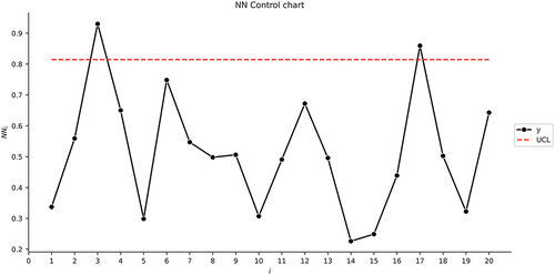The corresponding UCL values by using $\mathit{\alpha }$ = 0.005 and 5000 simulation runs are obtianed as 0.7686, 0.9644, and 0.8774, respectively, for the SVR, RFR, and NN control charts.

We can see similar behavior in Figures 1, 2 and 3. Four out-of-control samples are detected for each control chart in the same sample numbers: 1, 5, 18, and 19.

Figure 1. The SVR control chart for the first illustrative example.

Figure 2. The RFR control chart for the first illustrative example.

Figure 3. The NN control chart for the first illustrative example.

A Volcano–Eruption Study

For the Poisson distribution, we use the real data from Amiri et al. (2014) which shows Poisson regression profiles with the number of agglomerates that are ejected from a volcano in successive days. Agglomerates are large, coarse, rock fragments associated with a lava flow that are ejected during explosive volcanic eruptions. The response variable is represented by the number of agglomerates and the size of agglomerates is the explanatory variable. The data set is gathered in 68 successive days, and therefore we have 68 Poisson profiles each containing the observations for 20 levels of the explanatory variable. The matrix of the explanatory variables is defined as

$\mathit{X}=\left[\begin{array}{ccccc}1& 1& 1& ...& 1\\ 3& 6& 9& ...& 57\end{array}\right].$

The in-control parameters are ${\mathit{\beta }}_0={\left(6.6485,-0.1020\right)}^T$ with covariance matrix:

$\sum =\left[\begin{array}{cc}{{\sigma }_1}^2& {\sigma }_1{\sigma }_2\\ {\sigma }_1{\sigma }_2& {{\sigma }_2}^2\end{array}\right]=\left[\begin{array}{cc}0.0012& -0.0001\\ -0.0001& \mathit{\hspace{0.17em}}0.0001\end{array}\right],$

Therefore, ${\sigma }_1=0.0346$ and ${\sigma }_2=0.0100$. We again generate 20 profiles from the out-of-control process (a shift ${\delta }_1=0.5$ in the intercept). Again, based on the results of Section Simulation Studies, we design the control charts with a log link function and the first training method for the SVR and NN control charts and use the third training method for the RFR control chart. Assuming $\mathit{\alpha }$ = 0.005 and with 5000 simulation runs, the UCL values are obtained as 0.4233, 0.9637, and 0.8146, respectively, for the SVR, RFR, and NN control charts.

As can be seen in Figures 4–6, similar to Section A Drug–Response Study, the SVR and NN control charts behave similarly. However, in this example, only two out-of-control samples are detected for sample numbers 3 and 17. In addition, for the RFR control chart, we detected 2 out-of-control samples but in different sample numbers: 3 and 6.

Figure 4. The SVR control chart for the second illustrative example.

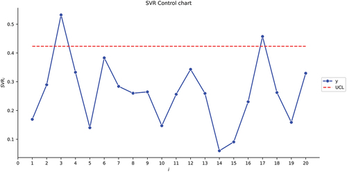
Figure 5. The RFR control chart for the second illustrative example.

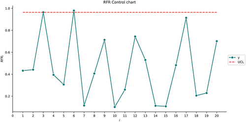
Figure 6. The NN control chart for the second illustrative example.

Concluding Remarks

In this paper, we developed the ML control charts for monitoring GLM-type profiles by considering different training methods, response distributions, and link functions. We first defined the GLM profiles for three main distributions: Binomial, Poisson, and Gamma with their corresponding link functions. Then, we described the ML techniques generally and then we moved on to the statistical and ML-based control charts.

A simulation study followed the theories. We trained the ML models and chose the best training method and ML control chart for the corresponding response distribution and link function. We considered three training methods with different shift sizes. For designing the control charts, we used the SVR, RFR, and NN techniques and compared the results using the ARL values.

In the case of Binomial profiles, for all link functions, we obtained the smallest values of ARL with the SVR and NN control charts and the first and second training methods depending on the shift sizes and types. For the Poisson profiles, with the log link function, the SVR control chart performed mostly the best with all the training methods except under simultaneous shifts. In that case, the NN control chart delivered the smallest values of ARL. For the sqrt link function, the SVR and NN control charts generally performed the best. In the case of shifts in the intercept, it was the NN control chart and the second training method, and under shifts in the slope, it was the SVR control chart and the first training method. Under simultaneous shifts, we also observed the smallest values of ARL with the SVR and NN control charts, and with the second training method. For the identity link function of Poisson profiles, we obtained the smallest values of ARL with the SVR control chart and the first training method, under shifts in the intercept. Under shifts in the slope, the NN control chart delivered the smallest values of ARL with the second training method, and under simultaneous shifts, it was a combination of the NN control chart with the second training method, and the SVR control chart with the first training method. For the Gamma profile with the log link function, the differences between the ARL values were negligible for the RFR and NN control charts. We obtained large values of ARL for almost all shift sizes in the case of the SVR control chart. For the identity link function, the NN control chart and all the training methods delivered the smallest values of ARL. For the Gamma profiles with the inverse link function, we obtained the smallest values with the SVR control chart and the second training method, and with the NN control chart and the third training method, depending on the type or size of the shifts. Furthermore, by approaching the results from a different perspective, it was clear that by keeping the ML technique and training method fixed, for the Binomial profile, using the probit link function emerged as the most effective (the smallest out-of-control ARL value) under most shift sizes and types, and in certain shift scenarios, the cloglog link function demonstrated superior performance, while the logit function proved to be the optimal choice in a few specific cases. For the Poisson profile, the log link function was the best in almost all the cases. For the Gamma profile, the findings exhibited greater diversity. In the case of the RFR and NN charts, the most effective link function was consistently the log link function. However, for the SVR chart, it was observed that the inverse link function predominantly outperformed others, followed by the identity function, and lastly, the log function.

It is important to acknowledge that employing an alternative simulation environment may yield varied results. In this study, we have solely examined outcomes within a singular simulation environment. To implement the proposed control charts in real practice, one may use the same method as we used in Section Simulation Studies to find the best combination of training method, and ML structure for the response distribution and link function to see which one results in better performance and use that control chart to monitor the process thereafter.

Finally, we presented illustrative examples to show how each ML control chart can be implemented in practice. The first example investigated the effect of a new pharmaceutical product in a dose–response study and the second example considered the number of agglomerates that were ejected from a volcano in successive days.

For future research, since in this paper it was assumed that the regression parameters’ values were known, one can consider performing this research in the case their values are unknown and should be estimated. In addition, different control charts can be developed and the results can be compared with the results of this paper.

Acknowledgements

The authors thank the journal’s editorial board and the reviewers for their constructive comments, which have led to significant improvements in the quality of the paper.

Disclosure Statement

No potential conflict of interest was reported by the author(s).

Data Availability Statement

The data that support the findings of this study are included in the paper.

Correction Statement

This article has been republished with minor changes. These changes do not impact the academic content of the article.

References

- Amiri, A., M. Koosha, and A. Azhdari. 2012. T2 based methods for monitoring Gamma profiles. Proceedings of The International Conference on Industrial Engineering and Operations Management, Istanbul, Turkey, 580–30.
- Amiri, A., M. Koosha, A. Azhdari, and G. Wang. 2014. Phase I monitoring of generalized linear model-based regression profiles. Journal of Statistical Computation and Simulation 85 (14):2839–59. doi:10.1080/00949655.2014.942864.
- Amiri, A., M. Mehrjoo, R. Ghajar, and F. Hosseini. 2010. Phase II monitoring of simple linear profiles under decreasing step shifts. Proceedings of The 40th International Conference on Computers & Industrial Engineering, 1–5. doi:10.1109/ICCIE.2010.5668258.
- Amiri, A., F. Sogandi, and M. Ayoubi. 2018. Simultaneous monitoring of correlated multivariate linear and GLM regression profiles in Phase II. Quality Technology & Quantitative Management 5 (4):435–58. doi:10.1080/16843703.2016.1226706.
- Apsemidis, A., S. Psarakis, and J. M. Moguerza. 2020. A review of machine learning kernel methods in statistical process monitoring. Computers & Industrial Engineering 142:1–12. doi:10.1016/j.cie.2020.106376.
- Boser, B. E., I. M. Guyon, and V. N. Vapnik. 1992. A training algorithm for optimal margin classifiers. Proceedings of the fifth annual workshop on Computational learning theory, 144–52. doi:10.1145/130385.130401.
- Breiman, L. 2001. Random Forests. Machine Learning 45 (1):5–32. doi:10.1023/A:1010933404324.
- Escobar, C. A., and R. Morales-Mendez. 2018. Machine learning techniques for quality control in high conformance manufacturing environment. Advances in Mechanical Engineering 10 (2):168781401875551. doi:10.1177/1687814018755519.
- Kang, L., and S. L. Albin. 2000. On-line monitoring when the process yields a linear profile. Journal of Quality Technology 32 (4):418–26. doi:10.1080/00224065.2000.11980027.
- Kim, K., M. A. Mahmoud, and W. H. Woodall. 2003. On the monitoring of linear profiles. Journal of Quality Technology 35 (3):317–28. doi:10.1080/00224065.2003.11980225.
- Koosha, M., and A. Amiri. 2011. The effect of link function on the monitoring of logistic regression profiles. Proceedings of the World Congress on Engineering, London, UK, vol. 1, 326–28.
- Koosha, M., and A. Amiri. 2013. Generalized linear mixed model for monitoring autocorrelated logistic regression profiles. The International Journal of Advanced Manufacturing Technology 64 (1–4):487–95. doi:10.1007/s00170-012-4018-2.
- Liaw, A., and M. Wiener. 2022. randomForest: Breiman and Cutler’s random forests for classification and regression. Accessed March 18, 2024. https://cran.rproject.org/web/packages/randomForest/index.html.
- Meyer, D. 2023. e1071: Misc functions of the department of statistics, probability theory group (formerly: E1071). TU Wien. Accessed March 18, 2024. https://cran.r-project.org/web/packages/e1071/index.html.
- Mohammadzadeh, M., A. Yeganeh, and A. Shadman. 2021. Monitoring logistic profiles using variable sample interval approach. Computers & Industrial Engineering 158:1–12. doi:10.1016/j.cie.2021.107438.
- Mohd Amiruddin, A. A. A., H. Zabiri, S. A. A. Taqvi, and L. D. Tufa. 2020. Neural network applications in fault diagnosis and detection: An overview of implementations in engineering-related systems. Neural Computing and Applications 32 (2):447–72. doi:10.1007/s00521-018-3911-5.
- Montgomery, D. C. 2012. Introduction to statistical quality control, 7th ed. AZ: John Wiley & Sons, Inc.
- Myers, R. H., D. C. Montgomery, G. G. Vining, and T. J. Robinson. 2010. Generalized linear models: with applications in engineering and the sciences, 2nd ed. Hoboken, New Jersey: John Wiley & Sons, Inc.
- Noorossana, R., A. Saghaei, and A. Amiri. 2011. Statistical analysis of profile monitoring. Hoboken, NJ: John Wiley & Sons.
- Olsson, U. 2002. Generalized linear models: an applied approach. Lund, Sweden: Studentlitteratur.
- Patterson, D. W. 1998. Artificial neural networks: Theory and applications, 1st ed. New Jersey, United States: Prentice Hall PTR.
- Qi, D., Z. Wang, X. Zi, and Z. Li. 2016. Phase II monitoring of generalized linear profiles using weighted likelihood ratio charts. Computers & Industrial Engineering 94:178–87. doi:10.1016/j.cie.2016.01.022.
- Ripley, B., and W. Venables. 2023. Nnet: Feed-forward neural networks and multinomial log-linear models. Accessed March 18, 2024. https://cran.r-project.org/web/packages/nnet/index.html.
- Sabahno, H., and A. Amiri. 2023. New statistical and machine learning based control charts with variable parameters for monitoring generalized linear model profiles. Computers & Industrial Engineering 184:1–18. doi:10.1016/j.cie.2023.109562.
- Sabahno, H., and S. T. A. Niaki. 2023. New machine-learning control charts for simultaneous monitoring of multivariate normal process parameters with detection and identification. Mathematic 11 (16):1–31. doi:10.3390/math11163566.
- Shadman, A., C. Zou, H. Mahlooji, and A. B. Yeh. 2014. A change point method for Phase II monitoring of generalized linear profiles. Communications in Statistics - Simulation and Computation 46 (1):559–78. doi:10.1080/03610918.2014.970698.
- Sharafi, A., M. Aminnayeri, and A. Amiri. 2013. An MLE approach for estimating the time of step changes in Poisson regression profiles. Scientia Iranica 20:855–60. doi:10.1016/j.scient.2012.10.043.
- Sogandi, F., and A. Amiri. 2015. Estimating the time of a step change in gamma regression profiles using MLE approach. International Journal of Engineering 28 (2):224–233. doi:10.5829/idosi.ije.2015.28.02b.08.
- Sogandi, F., and A. Amiri. 2017. Monotonic change point estimation of generalized linear model-based regression profiles. Communications in Statistics - Simulation and Computation 46 (3):2207–27. doi:10.1080/03610918.2015.1039132.
- Soleimani, P., R. Noorossana, and A. Amiri. 2009. Simple linear profiles monitoring in the presence of within profile autocorrelation. Computers & Industrial Engineering 57 (3):1015–21. doi:10.1016/j.cie.2009.04.005.
- Stoean, C., and R. Stoean. 2014. Support vector machines and evolutionary algorithms for classification: Single or together. Cham, Switzerland: Springer Publishing Company, Incorporated.
- Yeganeh, A., S. A. Abbasi, F. Pourpanah, A. Shadman, A. Johannssen, and N. Chukhrova. 2022. An ensemble neural network framework for improving the detection ability of a base control chart in non-parametric profile monitoring. Expert Systems with Applications 204:1–18. doi:10.1016/j.eswa.2022.117572.
- Yeganeh, A., S. A. Abbasi, S. C. Shongwe, J.-C. Malela-Majika, and A. Shadman. 2023. Evolutionary support vector regression for monitoring Poisson profiles. Soft Computing 28 (6):4873–97. doi:10.1007/s00500-023-09047-2.
- Yeganeh, A., N. Chukhrova, A. Johannssen, and H. Fotuhi. 2023. A network surveillance approach using machine learning based control charts. Expert Systems with Applications 219:1–17. doi:10.1016/j.eswa.2023.119660.
- Yeganeh, A., A. Johannssen, N. Chukhrova, S. A. Abbasi, and F. Pourpanah. 2023. Employing machine learning techniques in monitoring autocorrelated profiles. Neural Computing & Applications 35 (22):16321–40. doi:10.1007/s00521-023-08483-3.
- Yeganeh, A., A. Johannssen, N. Chukhrova, M. Erfanian, M. R. Azarpazhooh, and N. Morovatdar. 2023. A monitoring framework for health care processes using generalized additive models and auto-encoders. Artificial Intelligence in Medicine 146:102689. doi:10.1016/j.artmed.2023.102689.
- Yeganeh, A., A. Johannssen, N. Chukhrova, and M. Rasouli. 2024. Monitoring multistage healthcare processes using state space models and a machine learning based framework. Artificial Intelligence in Medicine 151:102826. doi:10.1016/j.artmed.2024.102826.
- Yeganeh, A., F. Pourpanah, and A. Shadman. 2021. An ANN-based ensemble model for change point estimation in control charts. Applied Soft Computing 110:1–19. doi:10.1016/j.asoc.2021.107604.
- Zou, C., Y. Zhang, and Z. Wang. 2006. A control chart based on a change-point model for monitoring linear profiles. IIE Transactions 38 (12):1093–103. doi:10.1080/07408170600728913.