Automatic Detection and 3D Reconstruction of Buildings from Historical Maps

ABSTRACT

This paper presents an automatic 3D building reconstruction methodology for historical urban maps. It uses facade and openings detection on the maps, followed by rectification, regularization, and 3D model generation techniques. Evaluation metrics confirm the effectiveness of the approach, with high accuracy in detecting facades and their openings while maintaining geometric integrity. The flexibility and interoperability of the chosen 3D building representation method allow for adjustments in dimensions without compromising layout, making it suitable for completing the urban environments where facades may not be directly visible. This methodology represents a significant step toward automating the reconstruction of 3D historical urban landscapes, contributing to heritage preservation and architectural understanding.

Introduction

In the past, maps played a fundamental role in bridging the gap between people and distant lands, offering a window to places beyond their immediate knowledge in times when global information was not available. Presently, these maps are regarded as invaluable historical documents, shedding light on historical perceptions of the world and enhancing our understanding of our place within it (Herold 2018). The study of historical urban maps is particularly revealing, as it allows for an in-depth analysis of city planning and architecture. By examining these maps, one can trace the influence of geographic, political, and environmental factors, as well as the progression of urbanization, providing a detailed overview of historical urban development practices.

For the study of urban elements in the past, it is necessary to make the information from historical maps accessible (Schlegel 2023). Manual attempts to acquire information from historical maps are not uncommon but error-prone, time-intensive, and nontransferable (Chiang et al. 2020; Gobbi et al. 2019; Xydas et al. 2022). Therefore, it is of interest to develop automated or semi-automated approaches to solve these problems.

Many techniques have been developed to extract 2D information from maps (Chiang, Leyk, and Knoblock 2014; Liu, Xu, and Zhang 2019), focusing on the extraction of linear features, such as streets (Chiang and Knoblock 2013) and rivers (Gede et al. 2020), area features like building footprints (Drolias and Tziokas 2020; Iosifescu, Tsorlini, and Hurni 2016; Riche 2020), land use classes (Gobbi et al. 2019; Zatelli et al. 2019), text (Pezeshk and Tutwiler 2011), and symbols or objects (Miao et al. 2017). Moreover, few studies have focused on large-scale but rather in small-scale maps (Gede et al. 2020; Heitzler and Hurni 2020; Herrault et al. 2013; Loran, Haegi, and Ginzler 2018).

The advent of deep learning has revolutionized the extraction of 2D information from maps, enabling the development of sophisticated models capable of recognizing and classifying diverse elements within spatial data. This not only streamlines the map analysis process but also opens new ways for extracting valuable information for various applications. In the context of our work, we will use deep learning for object detection in maps for understanding and extracting building facades, which serves as an initial step toward the automatic 3D reconstruction of buildings.

Applications of deep learning for 2D map processing arise in several fields (Uhl and Duan 2021). For example, in the extraction of linear features (Duan et al. 2018), a Convolutional Neural Network (CNN) model is tested for the recognition of several linear geographic elements from USGS historical topographic maps. An example for area features can be found in Jiao, Heitzler, and Hurni (2020), where a CNN is used to extract wetland areas from historical maps. In Heitzler and Hurni (2020), an ensemble of U-Net CNNs is used to extract building footprints from historical topographic maps from Switzerland, based on manually digitized training data, followed by a vectorization method that includes geometric refinement of the semantic segmentation results. Similarly, Xydas et al. (2022) study the extraction of building footprints using a U-Net architecture.

Regarding text features, in Li, Liu, and Zhou (2018), a framework is proposed for “topographic map understanding” that uses a CNN to localize and understand text elements in map documents. An example for symbol recognition can be found in Uhl (2019), where large amounts of settlement symbol data were collected in order to train a CNN for their recognition in maps from the United States Geological Survey (USGS).

In the specific case of information extraction from cadastral maps, which vary significantly from topographic maps in content and symbology (Ignjatić, Nikolić, and Rikalović 2018), presents an overview on deep learning methods. Specific cases include (Oliveira, Kaplan, and Lenardo 2017), where a CNN is employed in combination with unsupervised segmentation for the extraction and recognition of cadastral parcels and handwritten digits in historical cadastral maps. Another example is (Karabork and Aktas 2018; Liu et al. 2017) that use neural networks and CNNs for the vectorization of cadastral maps or floor plans, respectively.

These advancements converge with the evolution of three-dimensional (3D) city models, which have increasingly dominated visualization in recent decades (Billen et al. 2014), transitioning from the inherently 2D nature of traditional maps.

The shift to 3D models is motivated by the inherent advantages of 3D representations, which offer enhanced comprehensibility compared to traditional two-dimensional maps and drawings. This paradigm shift aligns with human perception of the world and facilitates improved communication and information sharing.

There have been several attempts to generate 3D models from 2D building footprints extracted from maps, marking a significant transition from 2D to 3D representations. Building heights, a first step in this transition, can be derived from existing information or estimated based on their attributes. For historical buildings that no longer exist, typical building heights can be inferred from historical documents or photographs. Beyond height, buildings can be further characterized by their roof shapes. For existing buildings, current data can be used, while historical information can be applied to non-existent structures. Finally, buildings can be textured on the roof surfaces and façades to achieve a more realistic representation. This can be done using existing texture databases or by creating new ones based on knowledge of typical façade and roof structures, as well as historically used materials.

Due to the reconstruction complexity, 3D building models available to the public often lack detailed representations, typically appearing as basic, solid structures with simplified roof shapes and textures (Balletti and Guerra 2016; Herold and Hecht 2017; Morlighem, Labetski, and Ledoux 2022; Neuhausen et al. 2018). Importantly, crucial elements, such as building openings (windows and doors) are frequently omitted.

The 3D reconstruction of existing buildings can also be obtained through direct measurement in the real world. This process commonly relies on 3D point clouds obtained by laser scanning or photogrammetry. These raw data must be further processed to obtain the individual components of the building (Arikan 2013; Holzmann 2017; Nan et al. 2015; Tomljenovic et al. 2015). However, due to the complexity of 3D point cloud processing, most reconstruction methods often overlook intricate building details.

Facade reconstruction from existing buildings relies mainly on photogrammetric techniques that generate detailed point clouds and textured models from a collection of photos (Xiao et al. 2009). However, many existing approaches require extensive manual pre- and post-processing, thereby limiting their viability as standalone solutions (Arikan 2013; Gruen et al. 2019; Nan et al. 2015).

These reconstructed buildings are often integrated into the creation of 3D models of historical cities. For example, the Roma Reborn project generated various versions of a virtual ancient Rome in 320 AD (Haegler, Müller, and Van Gool 2009). Similarly, a 3D model of the city of Prague was generated using an existing scale model (Sedlacek and Zara 2009). A 4D model of the city of Hamburg (Kersten et al. 2012) utilized data sources from a wooden model from 1644 and one of the first official plans of the city from 1859. A 3D recreation of the city of Nafplio in the nineteenth century was developed for an educational application. The authors addressed the challenge of modeling buildings that no longer exist today by integrating graphic documents such as photographs, drawings, and paintings, as well as buildings that have undergone interventions after the recreated period (Kargas, Loumos, and Varoutas 2019). A similar 3D reconstruction was presented for the city of San Cristóbal de La Laguna in (Pérez Nava et al. 2023). Besides visualization, these historical 3D models can be also used for city-scale augmented reality applications (Lee et al. 2012; Sánchez Berriel, Pérez Nava, and Albertos 2023).

In this paper, we study the possibility of 3D building detection and reconstruction from historical maps. This approach is a step toward more efficient ways to reconstruct historic 3D city models. Treating the ancient map as a modern plane or satellite image, we will first detect the building's facades. The facade is the principal face of the building, and its detection involves identifying and delineating the distinct elements like its openings that make up the external structure. This process is fundamental to understanding the geometry and structure of buildings, making it an essential step in the automated reconstruction of 3D models. The main challenge lies in the detection of buildings and the facade elements in the absence of 3D geometric information or coherence in the historical map. Traditional image processing techniques often struggle to handle these complexities, motivating the adoption of advanced methods, such as deep learning for more accurate and robust detection. The utilization of deep learning for facade detection is integral to the proposed approach, which will be detailed in the subsequent sections. The overarching goal is to leverage these advancements to automatically identify and extract building facades and their openings from historical maps, laying the groundwork for the subsequent stages of 3D reconstruction.

The main contributions of this paper are:

• Integration of Historical Maps for 3D Building Reconstruction: The paper introduces a novel approach by incorporating historical maps, specifically those of Leonardo Torriani in the “Description and History of the Kingdom of the Canary Islands,” into the process of 3D building reconstruction. This inclusion of historical cartographic data provides a unique source of information for enhancing the accuracy and completeness of the reconstructed buildings.

• Deep Learning-Based Facade and Openings Detection: The paper contributes to the field of object detection by employing deep learning techniques for the detection of buildings and facade elements in images. The proposed workflow involves the generation of a learning set and the application of deep learning algorithms to automatically identify and delineate building facades and openings from the input data. This automated detection process forms a crucial step in the overall 3D reconstruction methodology.

• Comprehensive Buildings Processing Workflow: The paper presents a detailed and comprehensive workflow for processing detected buildings facades, encompassing various stages such as facade detection, rectification, regularization, subdivision, and reconstruction. Each of these stages address specific challenges in the reconstruction process, ensuring the generation of accurate and visually realistic 3D models of buildings from the detected facades.

• Multi-Faceted Evaluation Metrics: The paper contributes to the assessment of the 3D reconstruction process by evaluating each step of the workflow using a set of standard metrics. Evaluation metrics are provided for the learning, rectification, regularization, and 3D generation processes. This approach allows for a detailed analysis of the proposed methodology, ensuring a comprehensive understanding of its performance and effectiveness.

Materials and Methods

In this section, we detail the materials and methods employed in our study. It encompasses two main subsections: the first focuses on the collection of historical maps that are used in our work and the second subsection outlines the detailed workflow for our 3D reconstruction process.

The Maps of Leonardo Torriani in the “Description and History of the Kingdom of the Canary Islands”

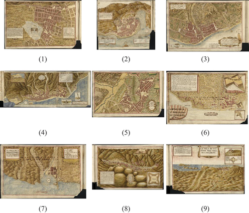
The cartographic collection utilized in this study was authored by the Italian engineer Leonardo Torriani. He was invited by the court of the Spanish King Felipe II to serve as a military engineer, spending a total of six years in the Canary Islands, divided into two periods starting in 1584. His tenure coincided with a period of increased strategic interest in the Canary Islands. During that time, Torriani meticulously documented the fortifications for the region, compiling extensive notes that culminated in his manuscript, “Description and History of the Kingdom of the Canary Islands” (Torriani 1590a). His book stands as an extraordinary historical and geographical contribution, offering a comprehensive portrayal of the Canary Islands during the sixteenth century. Torriani’s work delivers detailed geographical descriptions of each Canary island, providing readers with insights into landscapes, topography, and natural features, painting a vivid picture of the islands’ physical characteristics. A notable aspect of Torriani’s work is the significant emphasis placed on maps and cartography. His meticulous maps cover each island, offering detailed insights into geographical nuances, coastlines, mountains, and other noteworthy features. Additionally, Torriani’s book provides intricate descriptions of the cities and towns in the Canary Islands, including the maps of the main cities at that time: San Cristóbal de La Laguna, Las Palmas de Gran Canaria, Garachico, Santa Cruz de la Palma, and others (see Figure 1). These city maps not only present the urban layout of the cities and their buildings but also show important features such as squares, civil and religious buildings, and everyday elements like fountains, mills, or water troughs. This detailed description of the buildings in the city was not exclusive to Torriani’s work but was common in maps of that time (Braun 1965) as can be seen, for example, in the city plots of Madrid (Instituto Geográfico Nacional 2022) or Seville (Gordo and Zamudio 2019). High resolution images of Torriani’s maps in Figure 1 are available in (Torriani 1590b).

Figure 1. Maps used in this study: from top to bottom and left to right and numbered 1 to 9: San Cristóbal de La Laguna, Garachico, Las Palmas de Gran Canaria, Santa Cruz de La Palma, Telde, Santa Cruz de tenerife, San Sebastian de La Gomera, Betancuria and Teguise. High resolution images of the maps are available in (Torriani 1590b).

3D Reconstruction Workflow

The approach outlined is divided into several generic steps, designed for versatility across various map types. Rather than concentrating exclusively on developing a tailored solution for our specific maps, we have opted for generic processing at each stage. While adjustments to the internal processes of individual stages may be needed to accommodate other different maps, the overarching process remains consistent. The specific stages of this process are elaborated and detailed below, as shown in Figure 2.

1. Building detection: The map is explored, and the facades of the buildings present in it are detected.

2. Detection of facade openings: doors and windows. The detected facades from the previous step are explored to extract the openings.

3. Rectification of facades: Geometric distortions of the facades are corrected to obtain a representation invariant to such transformations.

4. Regularization: The geometric information obtained from the map is combined with a priori information about the arrangement of the facade elements and their metrics.

5. Generation of the 3D model of the facades: The generated facade is used to obtain a 3D model of the complete building.

Figure 2. Workflow of the 3D reconstruction process.

Building Detection

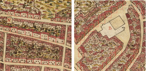
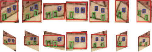
The successful application of deep learning models for building detection relies heavily on the availability of a representative learning set. To construct the learning set, we draw upon the historical maps in (Torriani 1590b) show in Figure 1. The first step involves the digitization of these historical maps to transform them into a format suitable for machine learning analysis. This digitization process has to be precise enough for the preservation of fine details and ensuring accurate representation of the building components. In our case, the digital reproduction of the maps was provided by the Library of the University of Coimbra (Portugal) where the original Torriani manuscript is conserved. Once digitized, the components of the dataset are 10 subimages of 640 × 640 pixels from each of the first 4 maps in Figure 1. Each subimage is manually annotated with ground truth information, indicating the location and boundaries of building facades within the images. Notice that our goal is to recover the frontal building facades so back-side facades or facades from inside the city blocks will not be in the learning set. To enhance the model’s ability to generalize, we employ data augmentation techniques, introducing variations such as rotation, shearing, scaling, and horizontal flipping to artificially expand the training dataset. This step is important for improving the model’s robustness to different scenarios and conditions. The learning set is divided into training and validation subsets for the subsequent deep learning-based facade detection model. Some elements in the training set are shown in Figure 3.

Figure 3. Elements in the learning set for facade detection. Bounding boxes for frontal facades are shown in red.

To detect the buildings in the image, we have employed the YOLOv8 model, built upon the YOLO (You Only Look Once) algorithm (Terven, Córdova-Esparza, and Romero-González 2023). YOLOv8 supports multiple-vision tasks, such as object detection, segmentation, pose estimation, tracking, and classification (Jocher, Chaurasia, and Qiu 2023).

The structure of the YOLOv8 network (see Figure 4) primarily comprises a backbone, neck, and head components. The backbone utilizes a modified CSPDarknet53 (Redmon and Farhadi 2018) as its basis, down sampling input features five times to produce five different scale features labeled in the Figure as P1–P5. The backbone network employs a C2f module in place of the original CSP module, enhancing detection accuracy by integrating high-level features with contextual information. This module performs convolution operations on input data, applies batch normalization, and activates the information stream using a Sigmoid-weighted Linear Unit (SiLU) to generate output results. Additionally, the backbone incorporates a spatial pyramid pooling fast (SPPF) module to pool input feature maps to a fixed-size map for adaptive size output.

Figure 4. Yolo v8 architecture (Range 2024).

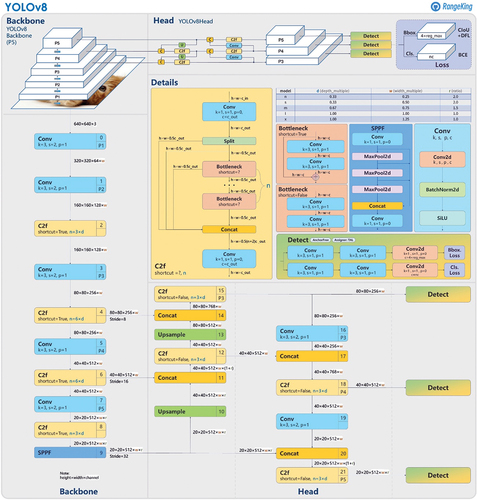
The neck structure of YOLOv8 is inspired by a Pyramid Attention Network (PANet) (Liu et al. 2018) and features a PAN-FPN (Path Aggregation Network with Feature Pyramid Network) configuration. This design mitigates scale variation issues in object detection by introducing a top-down pathway to build a feature pyramid, facilitating the effective capture of features across various scales. The PAN component further enhances the feature pyramid by introducing lateral connections that combine high-level semantic features from previous levels with low-level features from the current level, promoting better information flow across different scales.

Finally, the detection portion of YOLOv8 adopts a decoupled head structure comprising separate branches for object classification and predicted bounding box regression. Different loss functions, including binary cross-entropy loss (BCE Loss) for classification and distribution focal loss (DFL) (X. Li et al. 2020) and Complete IoU (CIoU) (Zheng et al. 2019) for bounding box regression, are employed to improve detection accuracy and model convergence. YOLOv8, being an anchor-free detection model, precisely defines positive and negative samples and utilizes the Task-Aligned Assigner (Feng et al. 2021) to dynamically assign data samples, further enhancing detection accuracy and model robustness.

Openings Detection

The detection of openings in facades plays a crucial role in various graphics and vision applications concerning 3D city modeling and scene visualization. Consequently, numerous methods have been devised for this purpose in real images (Lee and Nevatia 2004; C.-K. Li et al. 2020; Neuhausen and König 2018; Rahmani and Mayer 2022), including the use of a Yolov3 detector (Hu et al. 2020).

While doors and windows could theoretically be detected as additional classes within the YOLOv8 network discussed in the previous section, such an approach would detect openings beyond the limits of the targeted frontal facades identified in previous section. This method leads to a degradation in detection accuracy. To address this challenge, we have implemented a secondary YOLO network. This network operates on the same set of images as in the preceding section but employs a mask that covers the complement of the frontal facades. An illustrative example of these learning images is provided in Figure 5. This approach separates the building and opening detection steps making the proposed 3D reconstruction workflow more flexible.

Figure 5. Elements in the learning set for openings detection. Bounding boxes for doors and windows in frontal facades are shown in green and blue respectively.

Facade Rectification

Following the detection of building facades and their inner structure using deep learning, the next step in the 3D reconstruction workflow is facade rectification. Facade rectification aims to transform the detected facades from the 2D historical maps into a corrected frontal view, providing the basis for accurate and geometrically faithful 3D reconstruction. The rectification process involves correcting distortions introduced by factors, such as perspective, scale, and spatial variations in the historical maps, which can significantly affect the accuracy of subsequent 3D reconstruction efforts.

There are several methods, including transform estimation and image warping techniques, to rectify the facades from existing buildings and ensure they conform to a standardized, orthogonal representation. Many techniques use the idea that most man-made structures tend to be rectangular. Early approaches group edges to find rectangles on facades (Han and Zhu 2009; Micusik, Wildenauer, and Kosecka 2008). Most recent approaches target Manhattan-type scenes where buildings and objects align with three main orthogonal directions. In this perspective, parallel lines in each direction converge toward three vanishing points. In (Affara et al. 2016) facade images are rectified using RANSAC to estimate a homography that maps a large number of edges to vertical or horizontal lines. In (Wu, Frahm, and Pollefeys 2010) the symmetry of repeated structures on a facade is used to rectify them. Other approaches use different clustering methods to group vanishing pointsfor example, J-Linkage (Tardif 2009) or RANSAC (Wildenauer and Hanbury 2012). In (Liu 2011) the perspective transform is corrected with the help of two vanishing points estimated from line segments in image of the facade. In Neuhausen et al. (2018), the perspective transform is corrected by manually selecting four points in the façade, user intervention is also needed in Zhu et al. (2020). Several attempts have been made to use deep learning for detecting vanishing points in images. In Zhai, Workman, and Jacobs (2016), the AlexNet network is used to predict the horizon line as an angle and distance from the principal point. A more recent approach uses deep learning to assign scores to a Gauss sphere (Kluger et al. 2017).

To rectify the facades in Torriani’s maps we must study their representation since they are not taken from a camera. The city layout in Torriani’s maps is based on a geometric plan of the town to which the facades of the buildings and the internal distribution of the blocks have been added. The metrical accuracy of the geometric plan is high considering the time in which it was made (Nava et al. 2022).

To study how to give an approximate metric to the buildings in the city in the maps a set of tests have been performed. In the first place, we studied whether the length of bases of the buildings reflected its true length, or are shortened due to the angle of the street in the map denoted as α (see Figure 6). In that case, their lengths should depend on the street angle. We found that they are approximately independent (coefficient of determination R² <0.01). The dependence between building height and street angle was also explored to find that they are also approximately independent (R² <0.01). Finally, we studied the dependence of the building height and the position of the house in the map to find also that they are approximately independent (R² <0.01). Therefore, the width and height of the facades are approximately independent of the position and orientation of the buildings in the map.

Figure 6. Building over a facade of angle α.

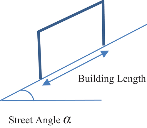
Then, to rectify the facade from a bounding box arising from its detection in a street with angle α, we must define a shearing transform with angle α and a scaling in the x direction to restore the true building length as seen in Figure 7.

Figure 7. Rectification process.

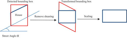
The overall effect for a bounding box with width w and height h, is a correction on its dimensions to a width of w/cos(α) and height of h - tan(|α|)w. The rectification transform T can be written as:

(1) $\mathit{T}=\left(\begin{array}{cc}1/\cos \left(\mathit{\alpha }\right)& 0\\ 0& 1\end{array}\right)\left(\begin{array}{cc}1& 0\\ -\tan \left(\mathit{\alpha }\right)& 1\end{array}\right)=1/\cos \left(\mathit{\alpha }\right)\left(\begin{array}{cc}1& 0\\ -\sin \left(\mathit{\alpha }\right)& \cos \left(\mathit{\alpha }\right)\end{array}\right)$(1)

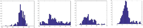
The same study was applied to doors leading to approximate independence of its dimensions with respect to angle (R² <0.01). However, for windows the best results were obtained by updating the positional information with the transform but keeping the original width and height of their bounding box since it generates an approximate independence of window dimensions with respect to angle (R² <0.01). This implies that there is a correlation between the bounding size rectification and its size that can be explained by the difficulty to correctly enclose windows with bounding boxes for increasing angles since they have around 7 pixels in the image.

After the previous transformations, the most straightforward way to provide an approximate metric to the buildings would be to use the map scale, either if it is provided or estimated. However, in our case, the scale of the buildings does not correspond to the scale of the map. For example, the approximate pixel size of Torriani’s map of San Cristóbal de La Laguna is 0.45 meters (Nava et al. 2022). Since doors in the map are around 11 pixels high this would lead to doors around 5 meters high and that is not the case. To provide an approximate metric for the buildings we set up a set of reference values for the sizes of doors and windows as seen in Table 1 (Nava et al. 2022). Then, for each house we compute the scaling factor of each element as the reference value divided by the number of pixels of the element. Finally, we collect all these measures and compute its weighted median with weights proportional to its pixel size to give a unique scaling value for each house.

Table 1. Reference values for the openings in the houses.

Door height	Door width	Window height	Window width
2.3	1.6	1.4	1.1

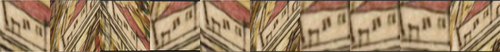
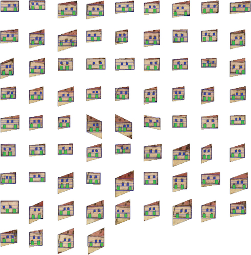
To finish with the rectification step, we need to show how to compute the shearing angle α. In our case, we have used a neural network to estimate α that has been trained with bounding boxes containing the facades and their true orientation. For each of these facades, we have generated an augmentation set warping each of the original images for random shearing angles in the interval [−60,60]. An example of such that augmentations is shown in Figure 8

Figure 8. Learning set augmentation.

The architecture of the orientation neural network is shown below in Figure 9:

Figure 9. Neural network architecture for shearing angle estimation.

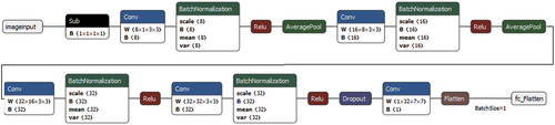
The network begins with eight convolutional filters, each followed by batch normalization and a ReLU activation function. This process is iteratively expanded with 16 and 32 filters to capture progressively intricate patterns. Average pooling is introduced for spatial reduction, and dropout is implemented to prevent overfitting during training. The final layer is fully connected for the prediction of the shearing angle. The model is trained with mean-squared-error loss.

Facade Regularization

After finishing the rectification of building facades, the next phase in our automated 3D reconstruction process involves facade regularization. This step aims to enhance the precision and coherence of the rectified facades, addressing the irregularities or distortions that may have arisen from the detection or rectification processes. Additionally, regularization helps to maintain the coherence of architectural elements within each facade, contributing to the overall visual consistency of the 3D reconstructed models. The regularization term acts as a form of prior knowledge, biasing the reconstruction process based on assumptions about the desired properties of the 3D model. In our case, very few building from Torriani’s time have survived so our prior knowledge arises mainly from the historical research of the city’s buildings (Cioranescu 1965; Navarro Segura 1999; Larraz Mora 2008).

Regularization methods can be classified into two categories: model and data-driven approaches. Model-driven methods typically employ grammar-based approaches to search for combinations from a predefined set of grammars while fitting relevant parameters (Teboul et al. 2013). However, optimizing these models can be a time-intensive and non-convergent process, particularly when the search space is vast (Tyleček and Šára 2013). While the model-driven approach can analyze a facade as a hierarchical structure, it is only feasible for examining regular facades due to its strict grammatical structure. For asymmetrical and misaligned facades, data-driven methods that account for weak architectural assumptions are more adaptable (Mathias, Martinović, and Van Gool 2016). Such methods lack clear grammatical definitions and usually represent windows and doors through their outer bounding boxes, which are then integrated into the facade layout. General constraints are applied to regularize the layout (Cohen et al. 2017; Hensel, Goebbels, and Kada 2019; Hu et al. 2020; Zhang and Aliaga 2022).

In our case, although the facades have a simple structure, the bounding boxes of the identified facade elements exhibit misalignment. Although there were irregular facades at that time (Larraz Mora 2008), in general we expect that windows on the same facade share uniform dimensions within a given row or column, showcasing alignment both horizontally and vertically. Our objective is to normalize the arrangement of windows and doors, aiming to make the facade modeling outcome closer to reality.

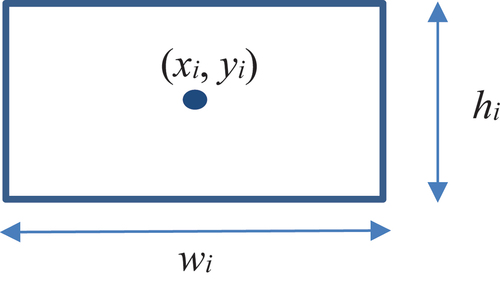
Given the initial result of the facade element detection and rectification, the layout comprises bounding boxes representing elements and can be denoted as L = {b₁, …b_n}. Each box b_i is characterized by its center coordinates (x_i, y_i), width and height dimensions (w_i, h_i), and the type of opening (door or window) (see Figure 10).

Figure 10. Facade bounding boxes after detection and rectification.

For most facades, we expect that the window layout follows a regular or semi-regular pattern, ensuring consistent distribution at the same level and column. Additionally, doors and windows should share identical dimensions, respectively. Expressing this prior knowledge of the facade layout involves a set of constraints, that regularize the result. Drawing inspiration from the methods in layout regularization (Jiang et al. 2016) our approach employs three types of constraints, namely same-size constraints, alignment and similar spacing to guarantee regularity in the final layout. The ultimate objective is to standardize the layout by treating it as an optimization problem, aiming to minimize alterations in box locations and sizes.

To enforce the same size constraints, we will define loss functions for the dimensions of doors and windows. For example, we use $\widetilde{w_h}$ as a prior value for window heights as defined in Table 1 and define the following loss function $E_{w_h}$ for the regularized value of the window height $\widehat{w_h}$

(2) $E_{\mathit{wh}}\left(\widehat{w_h}\right)=p_{\mathit{data}}\sum _{\mathit{i}=1}^n{\left(\widehat{w_h}\mathit{\hspace{0.17em}}-h_i\right)}^2+p_{\mathit{prior}}{\left(\widehat{w_h}\mathit{\hspace{0.17em}}-\widetilde{w_h}\right)}^2$(2)

where $\mathit{n}$ is the number of windows, $h_i$ is the detected value for the window height, $p_{\mathit{data}}$ is the precision of the data term and $p_{\mathit{prior}}$is the precision of the prior term. The first term considers the difference between the regularized height and the actual height, while the second measures the distance of the regularized height to the prior. Similar loss functions are defined for window width $E_{w_w}$ door width $E_{d_w}\mathit{\hspace{0.17em}}$and door height and $E_{d_h}$.

To enforce alignment constraints, we also define several loss functions. For example, for y-coordinate alignment, we proceed as follows. First, we cluster the y-coordinates of the centers of facade elements (door or window) $e_{y_i}$ into several clusters $G_1,\dots G_m$ (Khan et al. 2014) and define the following loss function for the regularized y-coordinates $\widehat{e_{y_i}}$ and clustered y-coordinates $\widetilde{e_{y_i}}$ that are equal to the mean of the $e_{y_i}$ coordinates for that cluster:

(3) $E_{G_y}\left(\widehat{e_{y_1}}\mathit{\hspace{0.17em}},\widehat{e_{y_2}}\mathit{\hspace{0.17em}},..,\widehat{e_{y_n}}\mathit{\hspace{0.17em}}\right)=\sum _{\mathit{i}=1}^m{E}_{G_i}\text{break}{E}_{G_i}=p_{\mathit{data}}\sum _{j\in G_i}^{\mathit{\hspace{0.17em}}}{\left(\widehat{e_{y_j}}\mathit{\hspace{0.17em}}-\widetilde{e_{y_i}}\right)}^2+p_{\mathit{constraint}}\sum _{j,k\in G_i}^{\mathit{\hspace{0.17em}}}{\left(\widehat{e_{y_j}}-\widehat{e_{y_k}}\right)}^2$(3)

where $\mathit{m}$ is the number of groups, $p_{\mathit{data}}$ is the precision of the data term and $p_{\mathit{constraint}}$ is the precision of the constraint term. The first term considers the difference between the regularized y-coordinates and the center of the y-cluster and the second ensures that each group $G_i$ is not broken by other loss functions. Similarly, another loss function $E_{G_x}$ is defined for the x-coordinates.

Finally, the last regularization term enforces same-spacing constraints between the facade elements. We will also define several loss functions. For example, for same spacing in x-coordinates we proceed as follows. We sort the x-coordinates and for each of the two boxes with x_j > x_i we check if they overlap in the y direction as shown in Figure 11.

Figure 11. Same spacing constraints.

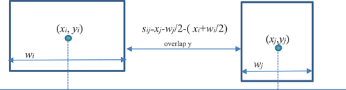
If they do, we compute their spacing s_ij as shown in Figure 11. Then, we cluster the pairwise spacings obtaining several groups (Khan et al. 2014) $H_1,\dots H_m$ and define the following loss function for the regularized x-coordinates $\widehat{e_{x_i}}$ and regularized width coordinates $\widehat{e_{w_i}}$ with clustered spacings coordinates $\widetilde{e_{x_i}}$equal to the mean of the spacings for that cluster:

(4) $\begin{array}{l}{E}_{\mathit{Hx}}\left(\widehat{e_{x_1}},\widehat{e_{x_2}},\mathrm{..},\widehat{e_{x_n}},\widehat{e_{w_1}},\widehat{e_{w_2}},\mathrm{..},\widehat{e_{w_n}}\right)={\displaystyle \sum _{\mathit{i}=1}^m{E}_{H_i}}\\ E_{H_i}=p_{\mathit{spacing}}{\displaystyle \sum _{\begin{array}{l}\left(\mathit{j},\mathit{k}\right)\in G_i\\ \widehat{e_{x_k}}-\widehat{e_{x_j}}>0\end{array}}{\left(\widehat{e_{x_k}}-\widehat{e_{x_j}}-\frac{\widehat{e_{w_k}}-\widehat{e_{w_j}}}{2}-{\tilde{e}}_{x_i}\right)}^2}\end{array}$(4)

where $\mathit{m}$ is the number of groups, $p_{\mathit{spacing}}$ is the precision of the spacing data term. The $E_{H_i}$ term takes into account the difference between the regularized x and w coordinates two overlapping boxes in y coordinates. Similarly, a loss function can be defined for the y coordinate $E_{\mathit{Hy}}$.

By adding all the loss terms we have the total loss $E_{\mathit{total}}=E_{\mathit{ww}}+E_{\mathit{wh}}+E_{\mathit{dw}}+E_{\mathit{dh}}+E_{\mathit{Gx}}+E_{\mathit{Gy}}+E_{\mathit{Hx}}+E_{\mathit{Hy}}$ that is quadratic in the regularized values for centers and sizes of the boxes and can be solved by standard optimization libraries (Harris et al. 2020).

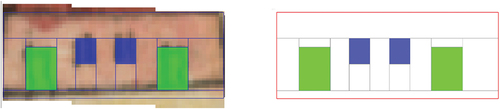
After the regularized values are computed for the inner elements of the facade, we define regularized values for the exterior of the facade using the previous elements by computing their bounding box and adding a border of L values as shown in Figure 12.

Figure 12. Facade exterior regularization.

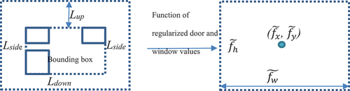
Then, the regularized values for the facade are computed from:

(5) $E_f=p_{\mathit{data}}\left({\left(\widehat{f_w}-f_w\right)}^2+{\left(\widehat{f_h}-f_h\right)}^2+{\left(\widehat{f_x}-f_x\right)}^2+{\left(\widehat{f_y}-f_y\right)}^2\right)+p_{\mathit{reg}}\left({\left(\widehat{f_w}-\widetilde{f_w}\right)}^2+{\left(\widehat{f_h}-\widetilde{f_h}\right)}^2+{\left(\widehat{f_x}-\widetilde{f_x}\right)}^2+{\left(\widehat{f_y}-\widetilde{f_y}\right)}^2\right)$(5)

The $\hat{f}$ variables are the regularized values of the box, the $\widetilde{f_x}$ variables act as a prior and the f values are the actual values of the facade exterior. The solution of (5) can be easily computed analytically.

Facade Representation

After the regularization of the facade, we are ready for 3D reconstruction. It is important to choose a 3D representation method that has some level of flexibility. We may want to adjust the house dimensions without altering its layout or we may want to generate other houses to complete the city for parts of the map where facades are not visible. In our case, we have selected a rule-based model (ArcGIS CityEngine 2023; Müller et al. 2006; Prusinkiewicz and Lindenmayer 1990; Stiny 1975). This modeling framework allows designers to create complex environments more quickly and parametrically compared to traditional methods. Their basis is the use of procedural rules and parameterization that describe how the elements of the model should be generated and organized. Rule parameters allow for easy adjustment of dimensions, shapes, and other attributes of 3D objects. This facilitates rapid iteration in design. Changes in rules and parameters are immediately reflected in the model, allowing designers to efficiently explore different options. Then, in the urban modeling context, much of the modeling process can be automated. This reduces manual workload and speeds up the creation of complex 3D models while maintaining consistency in design and model quality. Finally, rule-based 3D models are compatible with other systems and data formats, facilitating integration with GIS tools, other 3D modeling software, or 3D renderers.

To define the set of rules that generate a particular facade, it must be divided into smaller elements. The subdivision process is guided by the building layout, ensuring that the resulting segments align with their inner elements. In our case, we will use the open source Shape Modeling Language (SML) (Lienhard 2024). The facades will be generated in terms of the split operators of the language. For example, given the box in Figure 13 composed of wall and windows:

Figure 13. Splitting of a box in the x-direction.

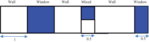
It can be split into subboxes in the x- direction by the splitX rule in SML defined as:

where the “sfsfsf” string means that the subbox is “(s)tretchable” or “(f)ixed” when reparametrizing the building. The underscore after Wall or Window means that those symbols are terminal, that is, their boxes have no inner structure. The symbol Mixed is non-terminal and will call for another split rule to follow the subdivision process.

To subdivide the house layout, we proceed in the y and x directions alternatively generating always in each direction the maximal subdivision (the one that generates more subboxes). An example of the whole process is shown in Figure 14.

Figure 14. Example of the subdivision process.

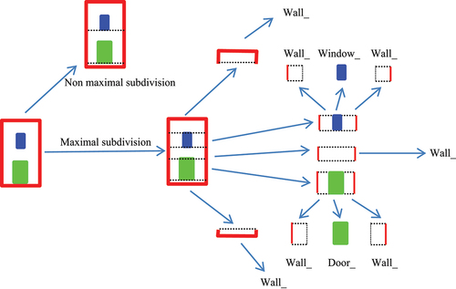
Facade subdivision, with its emphasis on generating procedural rules, bridges the gap between detected facades and the creation of complex, context-aware 3D models, since we can easily attach to the terminal door or window boxes any detailed external 3D model thereby enhancing the realism and historical fidelity of the reconstructed city.

Results

In this section, we present the results of our work, focusing on various evaluation metrics applied to different processes. We begin by examining the evaluation metrics employed to assess the effectiveness of the detection process, followed by a similar analysis for the rectification and regularization processes. Finally, we detail the evaluation of the reconstruction process, providing insights into its performance and efficacy.

Evaluation metrics of the detection process

This section outlines the evaluation metrics employed to assess the performance of the deep learning model during the training phase, utilizing the learning set generated from the historical maps of Leonardo Torriani. We used the YOLOv8n model developed by Ultralytics, version 0.196. The experimental environment was configured using Python 3.1220, VScode (1.87) IDE, and CUDA 12.3. All model training and validation were executed on an NVIDIA GeForce RTX 3060 (12 GB). During the training phase, the Adam optimizer was used with learning rate 0.001, and momentum 0.9. The decay was set to 0.0005. The entire model-training process was fast and spanned approximately 5 minutes. Precision and recall exhibited a quick learning trajectory during the 100 training iterations, encountered initial periodic fluctuations in precision, and attained stability after 80 iterations.

To verify the efficacy of the modified YOLOv8n model, using our datasets, we used four metrics: Precision, Recall, F1 Score, and mAP., complemented by the confusion matrix. These metrics provide a comprehensive understanding of the model’s performance. Precision measures the accuracy of positive predictions, recall assesses the model’s ability to capture all relevant instances, and the F1 score combines both precision and recall, offering a balanced measure of the model’s overall effectiveness. An Intersection Over Union (IOU) threshold of 0.5 and a confidence threshold of 0.1 for houses and 0.25 for openings were established to assess experimental outcomes. The learning set was taken from the first four images in Figure 1 and divided into training (70%) and validation data (30%). The results on the validation data are shown in Table 2.

Table 2. Results of the detection process.

Detection	Precision	Recall	mAP@0.5	mAP@0.5:0.95	F1-score
Houses	0.97	0.93	0.97	0.77	0.94
Openings	0.97	0.97	0.98	0.56	0.97

The model’s performance in object detection is noteworthy for the two distinct classes, “Houses” and “Openings.” For “Houses,” the model demonstrates a very high precision (97%) and recall (93%), resulting in a well-balanced F1-score of 94%. The high [email protected] of 97% accentuates the model’s accuracy in localizing “Houses,” and the [email protected]:0.95 drops to 77%. Similarly, for “Openings” the model showcases remarkable precision (97%) and recall (97%), yielding a robust F1-score of 97%. The [email protected] of 98% highlights precise localization, and the [email protected]:0.95 experiences a decrease to 56%. Overall, the model detects both classes with high precision and recall, demonstrating its proficiency in object localization tasks. The F1 versus confidence curve (Figure 15) shows the F1 score of the model at different confidence thresholds.

Figure 15. F1 curve for houses and openings.

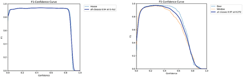
As can be seen in previous images, the F1 curve for the house model is consistently above 0.9 being indicative of a robust performance in correctly identifying and localizing objects in the given dataset. The F1 curve for the openings also obtains high values being slightly higher for doors than for windows. The confusion matrix is shown in Table 3, where the left table is for houses, and the right table is for openings.

Table 3. Confusion matrix for houses and openings.

				Detected	Door	156	0	4
Detected	House	224	14		Window	0	184	5
	Background	20	0		Background	3	6	0
		House	Background			Door	Window	Background
True					True

Results show that from the 244 houses that were present in the validation set 92% were correctly identified, while 20 houses were not identified. There were 14 doors identified in the background. On the other hand, from the 159 doors on the validation set, 98% were correctly identified and 3 were not identified, from the 190 windows 97% were correctly identified and 6 were not identified. There were 5 windows and 4 doors identified in the background. Some graphical results for the detection process are shown in Figure 16.

Figure 16. Detection results of frontal facades for the map of San Cristóbal de La Laguna.

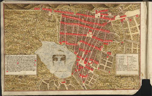
The total number of detected frontal facades in each map is shown in Table 4.

Table 4. Number of detected frontal facades in maps 1–4.

San Cristóbal de La Laguna	294	Garachico	260
Las Palmas de Gran Canaria	215	Santa Cruz de La Palma	382

In another set of experiments, we studied the generalization capability of the model to other maps from Torriani’s work. We applied the learned model to the maps of the village of Telde, Santa Cruz de Tenerife and Sebastian de la Gomera (maps 5–7). All the previous maps share the features of the learning set (maps 1–4), that is, a map seen from above where houses are drawn over the block’s limits, but also have some differences like city extent or number of houses in rural areas. The results for house detection are shown in Table 5.

Table 5. Detection results for test maps 5–7.

Map	Precision	Recall %	mAP@0.5	mAP@0.5:0.95	F1-score
Telde	0,85	0,88	0.82	0.56	0,87
San Sebastian	0,92	0,85	0.92	0.60	0.88
Santa Cruz	0,94	0,85	0.90	0.73	0,89

The [email protected] values for the openings in the previous maps were 0.83, 0.99 and 0.93, respectively. The number of detected facades in each map is shown in Table 6.

Table 6. Number of detected frontal facades in maps 5–9.

Telde	188	Santa Cruz de Tenerife	96
San Sebastián de La Gomera	11	Betancuria	45
Teguise	13

Evaluation metrics of the rectification process

The rectification of building facades is the next step in our automatic 3D reconstruction methodology, influencing the accuracy and geometric fidelity of subsequent stages. The experimental environment was the same as the previous section. During the training phase for the angle estimation network, the Adam optimizer was used with learning rate 0.001, and momentum 0.9. The decay was set to 0.0005. The entire training process was fast and spanned approximately 5 minutes. Loss and Root Mean Square Error (RMSE) exhibited a quick learning trajectory during the 2000 training iterations, encountered initial descent, and attained stability after 1000 iterations.

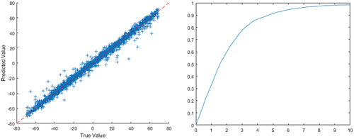
The RMSE over the validation set was 3.33 degrees. As can be seen from Figure 17 (left), prediction errors are mostly the same over all the angular range. In Figure 17 (right), it is shown the percentage of images whose error is below a predetermined threshold. It can be seen that 90% of images have an error below 4.8 degrees and 95% of images below 6.3 degrees.

Figure 17. Rectification errors.

The estimated angular distribution in the maps 1–4 in Figure 1 is shown below in Figure 18.

Figure 18. Estimated angular distribution of houses in maps 1–4.

Below, we show in Figure 19 some qualitative examples of the rectification process. As can be seen, the map distortion is mostly corrected.

Figure 19. Results of the rectification process.

Evaluation metrics of the regularization process

The regularization of building facades is the next step in the 3D reconstruction methodology. Since regularization precedes 3D reconstruction, we have chosen a visual quality assessment that involves a qualitative evaluation of the regularized facades. A comparative analysis between the original and regularized facades allows for a subjective judgment of the visual plausibility of the reconstruction process.

We began by assembling a random collection of 50 original house images, detected and rectified from maps 1–4, to ensure that the evaluation could capture the variability in houses layout. Following image selection, we applied the regularization technique described in Section 2.2.4 to transform the original house images into a regularized layout.

To obtain user feedback, we developed a user-friendly interface where participants could evaluate pairs of images side by side. Each pair comprised an original image in the map and its corresponding regularized version (see Figure 20). Ten participants were then asked to assign scores to the image pairs based on the perceived number of errors in the final layout. The assigned values were 0 for all errors, 1 for many errors, 2 for some errors and 3 for error-free. The collected scores were then analyzed to obtain feedback about the regularization process.

Figure 20. Evaluation of the regularization process.

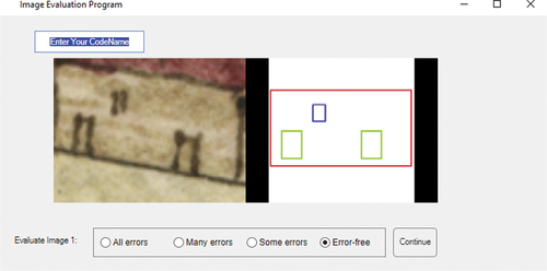
The average score obtained was of 2.75 out of 3 and a standard deviation of 0.07. This high score close to the maximum suggests that the technique aligns well with human perceptions of visual accuracy and plausibility. The low standard deviation indicates a consensus among participants, reinforcing the technique’s effectiveness across different building facades and layouts.

Evaluation of the reconstruction process

The effectiveness of the 3D reconstruction method was evaluated in terms of flexibility and interoperability. As explained before, the rule-based model was selected for its ability to offer a certain level of flexibility in representing facades. This flexibility is crucial as it allows for adjustments in house dimensions without compromising the layout and enables the generation of additional houses to complete urban environments where facades are not directly visible. Furthermore, the rule-based model’s reliance on procedural rules and parameterization facilitates rapid iteration in design. The whole process begins with the automatic subdivision shown in Figure 14. An example of its results is shown in Figure 21.

Figure 21. Example of the automatic subdivision process.

After facade partitioning, the ShapeML procedural rules that describe the facade are automatically generated. An example of the set of houses generated by a particular rule is shown in Figure 22.

Figure 22. Example of the facades generated by a particular procedural rule over imposed over the regularized house image.

Using the procedural modeling, designers can easily adjust dimensions (see the red square in the left image of Figure 23), shapes, or other attributes of the facade like textures through rule parameters leading to efficient adjustment of design. Other geometric parameters, such as house width, roof angle and roof type are estimated from historical sources (Larraz Mora 2008). Textures for all the house elements have been generated from houses with the same construction techniques in the city.

For virtual reality applications, where users navigate through the city, back facades are typically not generated since they are not visible during normal navigation. However, they may become necessary for generating an aerial view of the city. As obtaining both frontal and back facades simultaneously from the map is not feasible, a straightforward solution is to generate back facades from the frontal facades by randomly changing some openings for walls.

Figure 23. 3D model generation using rule-based models for the house in Figure 22.

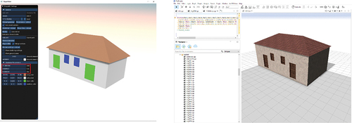
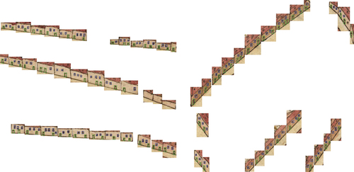
Another aspect to evaluate for the 3D reconstruction model is the capacity to interoperate with other systems for 3D generation. Since all the information for 3D generation is integrated into procedural rules, it is feasible to transfer them between similar systems. For example, in Figure 23 (left) we show the same set of rules applied in ShapeMaker (Lienhard 2024) and the rule-based CityEngine (ArcGIS CityEngine 2023) system (right). Moreover, the ability to export the 3D reconstruction in multiple formats facilitates seamless integration with GIS tools, other 3D modeling software, or 3D renderers, enabling interdisciplinary collaboration and data exchange. This capability is demonstrated in Figure 24, where a subset of the detected houses is made available to the designer in the open-source program Blender. Additionally, in Figure 25, the house from Figure 23 is integrated into a complex scene in Blender, while Figure 26 shows the first row of houses from Figure 24 joined along one side of a street in another Blender scene.

This automation inherent in rule-based modeling reduces manual workload and expedites the creation of complex city 3D models while ensuring consistency in design and model quality.

Figure 24. Subset of the houses available to the 3D designer.

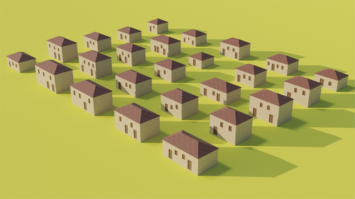
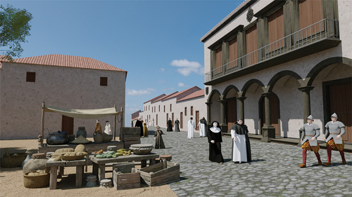
Figure 25. House of Figure 23 integrated in a complex scene.

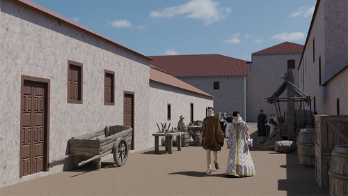
Figure 26. First row of house of Figure 24 besides an administrative building in the city.

Conclusions

In this study, we presented an automatic 3D building reconstruction methodology tailored for historical urban landscapes, using facade detection, rectification, regularization and 3D generation. The application of this methodology to the historical maps of Leonardo Torriani in the “Description and History of the Kingdom of the Canary Islands” aimed to provide a precise and detailed reconstruction of the building facades.

The evaluation metrics applied to each stage of the methodology show the effectiveness of the proposed approach. During the learning process, the deep learning model exhibited high precision, recall, and F1 score, indicating its capability to detect building facades and openings accurately. The rectification process maintained geometric accuracy, and the regularization process succeeded in ensuring a visually coherent representation.

The effectiveness of the 3D reconstruction method was assessed based on its flexibility and interoperability. The chosen rule-based model demonstrated significant flexibility in representing facades, allowing for adjustments in house dimensions without compromising the layout. This flexibility is crucial for generating additional houses to complete urban environments where facades are not directly visible. Additionally, the reliance on procedural rules and parameterization facilitates rapid iteration in design.

The findings of this study suggest that our automatic 3D reconstruction methodology is an effective approach for generating historically faithful 3D models of buildings from map facades. The presented methodology can be applied in heritage dissemination, 3D urban reconstruction or historical research.

However, there are some limitations and challenges. The neural network model was only trained on city images and did not give good results on detecting houses in maps of rural areas (maps 8–9 in Figure 1). The model also had some difficulties to detect some house types not present in the learning set. Finally, due to the high number of generated houses, a clustering of the reconstructed buildings into classes would help the 3D designer to choose the most suitable one. Future work may focus on refining the methodology to address these challenges, testing additional datasets, explore the automatic placement of houses in the city and expanding the applicability to different historical contexts.

In conclusion, the presented methodology represents a significant step toward automating the reconstruction of 3D historical urban landscapes. By integrating advanced computational techniques with historical maps, we contribute to the broader goals of preserving cultural heritage and fostering a deeper understanding of architectural evolution in historical contexts.

Disclosure Statement

No potential conflict of interest was reported by the author(s).

Data Availability Statement

The data that support the findings of this study are available from the corresponding author, F.P.N, upon reasonable request.

References

- Affara, L., L. Nan, B. Ghanem, and P. Wonka. 2016. Large scale asset extraction for urban images. Proceedings of the European Conference on Computer Vision, Amsterdam, Netherlands, 437–34.
- ArcGIS CityEngine. 2023. Computer Software. ESRI, 1. https://www.esri.com/es-es/arcgis/products/arcgis-cityengine/overview.
- Arikan, M. 2013. O-Snap: Automatic polygonal reconstruction with interactive refinement. [Publisher Name].
- Balletti, C., and F. Guerra. 2016. Historical maps for 3D digital city’s history. Cartographica: The International Journal for Geographic Information & Geovisualization 51 (3):115–26. doi:10.3138/cart.51.3.3140.
- Billen, R., A.-F. Cutting-Decelle, O. Marina, J.-P. De Almeida, M. C. G. Falquet, T. Leduc, C. Métral, G. Moreau, J. Perret, et al. 2014. 3D city models and urban information: Current issues and perspectives: European COST action TU0801. In 3D city models and urban information: Current issues and perspectives – European COST action TU0801, ed. R. Billen and S. Zlatanova, I–118. Les Ulis, France: EDP Sciences. doi:10.1051/TU0801/201400001.
- Braun, G. 1965. Civitates orbis terrarum (vols. 1 and 2). apud auctores.
- Chiang, Y., W. Duan, S. Leyk, J. Uhl, and C. Knoblock. 2020. Using historical maps in scientific studies: Challenges and best practices. Cham, Switzerland: Springer. doi:10.1007/978-3-319-66908-3.
- Chiang, Y. Y., and C. A. Knoblock. 2013. A general approach for extracting road vector data from raster maps. IJDAR 16 (1):55–81. doi:10.1007/s10032-011-0177-1.
- Chiang, Y.-Y., S. Leyk, and C. A. Knoblock. 2014. A survey of digital map processing techniques. ACM Computing Surveys 47 (1):1–44. doi:10.1145/2557423.
- Cioranescu, A. 1965. La Laguna: Guía histórica y monumental. San Cristobal de La Laguna: Ayuntamiento de San Cristobal de la Laguna.
- Cohen, A., M. R. Oswald, Y. Liu, and M. Pollefeys. 2017. Symmetry-aware façade parsing with Occlusions. 2017 International Conference on 3D Vision (3DV), 393–401. doi:10.1109/3DV.2017.00052.
- Drolias, G. C., and N. Tziokas. 2020. Building footprint extraction from historic maps utilizing automatic vectorisation methods in open source GIS software. Automatic Vectorisation of Historical Maps: International Workshop Organized by the ICA Commission on Cartographic Heritage into the Digital. Budapest – 13 March, 2020, 9–17. doi:10.21862/avhm2020.01.
- Duan, W., Y.-Y. Chiang, C. A. Knoblock, S. Leyk, and J. H. Uhl. 2018. Automatic generation of precisely delineated geographic features from georeferenced historical maps using deep learning. The 22nd International Research Symposium on Computer-Based Cartography and GIScience (Autocarto/UCGIS). https://www.ucgis.org/assets/docs/AutoCarto-UCGIS%202018%20Proceedings.pdf.
- Feng, C., Y. Zhong, Y. Gao, M. R. Scott, and W. Huang. 2021. TOOD: Task-aligned one-stage object detection. CoRR, abs/2108.07755.
- Gede, M., V. Árvai, G. Vassányi, Z. Supka, E. Szabó, A. Bordács, C. G. Varga, and K. Irás. 2020. Automatic vectorisation of old maps using QGIS – tools, possibilities and challenges. In Automatic vectorisation of historical maps, ed. I. Krisztina, 39–45. Budapest: ELTE Eötvös Loránd University.
- Gobbi, S., M. Ciolli, N. La Porta, D. Rocchini, C. Tattoni, and P. Zatelli. 2019. New tools for the classification and filtering of historical maps. ISPRS International Journal of Geo-Information 8 (10):455. doi:10.3390/ijgi8100455.
- Gordo, A. G., and T. D. Zamudio. 2019. Sevilla extramuros en el siglo XVI: tres vistas del Civitates Orbis Terrarum. Boletín de la Asociación de Geógrafos Españoles 80:1–28.
- Gruen, A., S. Schubiger, R. Qin, G. Schrotter, B. Xiong, J. Li, X. Ling, C. Xiao, S. Yao, and F. Nuesch. 2019. Semantically enriched high resolution LOD 3 building model generation. International Archives of the Photogrammetry, Remote Sensing and Spatial Information Sciences XLII-4/W15:11–18. doi:10.5194/isprs-archives-XLII-4-W15-11-2019.
- Haegler, S., P. Müller, and L. Van Gool. 2009. Procedural modeling for digital cultural heritage. EURASIP Journal on Image and Video Processing 2009:1–1. doi:10.1155/2009/852392.
- Han, F., and S.-C. Zhu. 2009. Bottom-up/top-down image parsing with attribute grammar. IEEE Transactions on Pattern Analysis & Machine Intelligence 31 (1):59–73. doi:10.1109/TPAMI.2008.65.
- Harris, C. R., K. J. Millman, S. J. Van Der Walt, R. Gommers, P. Virtanen, D. Cournapeau, E. Wieser, J. Taylor, S. Berg, N. J. Smith, et al. 2020. Array programming with NumPy. Nature 585 (7825):357–62. doi:10.1038/s41586-020-2649-2.
- Heitzler, M., and L. Hurni. 2020. Cartographic reconstruction of building footprints from historical maps: A study on the Swiss Siegfried map. Transactions in GIS 24 (2):442–61. doi:10.1111/tgis.12610.
- Hensel, S., S. Goebbels, and M. Kada. 2019. Facade reconstruction for textured lod2 citygml models based on deep learning and mixed integer linear programming. ISPRS Annals of the Photogrammetry, Remote Sensing & Spatial Information Sciences 4:37–44. doi:10.5194/isprs-annals-IV-2-W5-37-2019.
- Herold, H. 2018. Geoinformation from the past. Springer Fachmedien Wiesbaden. doi:10.1007/978-3-658-20570-6.
- Herold, H., and R. Hecht. 2017. 3D reconstruction of urban history based on old maps. In Digital research and education in architectural heritage, ed. S. Munster, 63–79. Cham, Switzerland: Springer.
- Herrault, P. A., D. Sheeren, M. Fauvel, and M. Paegelow. 2013. Automatic extraction of forests from historical maps based on unsupervised classification in the CIELab color space. In Geographic information science at the heart of Europe: Lecture notes in Geoinformation and cartography, ed. D. Vandenbroucke, B. Bucher, and J. Crompvoets. Springer. doi:10.1007/978-3-319-00615-4_6.
- Holzmann, T. 2017. Hybrid method for 3D and plane-based Urban Reconstruction. [Publisher Name].
- Hu, H., L. Wang, M. Zhang, Y. Ding, and Q. Zhu. 2020. Fast and regularized reconstruction of building faÇades from street-view images using binary integer programming. ISPRS Annals of the Photogrammetry, Remote Sensing & Spatial Information Sciences V-2-2020:365–71. doi:10.5194/isprs-annals-V-2-2020-365-2020.
- Ignjatić, J., B. Nikolić, and A. Rikalović. 2018. Deep learning for historical cadastral maps digitization: Overview, challenges and potential. https://otik.uk.zcu.cz/handle/11025/34636.
- Instituto Geográfico Nacional. 2022. Madrid. Planos de población. (1656). 1881. Instituto Geográfico Nacional - Servicio de Documentación, January 13. https://www.ign.es/web/catalogo-cartoteca/resources/html/001488.html.
- Iosifescu, I., A. Tsorlini, and L. Hurni. 2016. Towards a comprehensive methodology for automatic vectorization of raster historical maps. E-Perimetron 11:57–76.
- Jiang, H., L. Nan, D.-M. Yan, W. Dong, X. Zhang, and P. Wonka. 2016. Automatic constraint detection for 2D layout regularization. IEEE Transactions on Visualization and Computer Graphics 22 (8):1933–44. doi:10.1109/TVCG.2015.2480059.
- Jiao, C., M. Heitzler, and L. Hurni. 2020. Extracting wetlands from Swiss historical maps with convolutional neural networks. In Automatic vectorisation of historical maps, ed. I. Krisztina, 33–38. Budapest: ELTE Eötvös Loránd University.
- Jocher, G., A. Chaurasia, and J. Qiu. 2023. Ultralytics YOLOv8 (8.0.0) [computer software]. https://github.com/ultralytics/ultralytics.
- Karabork, H., and E. Aktas. 2018. The international archives of the photogrammetry, remote sensing and spatial information sciences. 1716–23.
- Kargas, A., G. Loumos, and D. Varoutas. 2019. Using different ways of 3D reconstruction of historical cities for gaming purposes: The case study of Nafplio. Heritage 2 (3):1799–811. Article 3. doi:10.3390/heritage2030110.
- Kersten, T. P., F. Keller, J. Saenger, and J. Schiewe. 2012. Automated generation of an historic 4D city model of Hamburg and its visualisation with the GE engine. Euro-Mediterranean Conference, Lemessos, Cyprus, 55–65.
- Khan, K., S. U. Rehman, K. Aziz, S. Fong, and S. Sarasvady. 2014. DBSCAN: Past, present and future. The Fifth International Conference on the Applications of Digital Information and Web Technologies (ICADIWT 2014), 232–38. https://ieeexplore.ieee.org/abstract/document/6814687/.
- Kluger, F., H. Ackermann, M. Y. Yang, and B. Rosenhahn. 2017. Deep learning for vanishing point detection using an inverse gnomonic projection. Proceedings of the German Conference on Pattern Recognition, Basel, Switzerland, 17–28.
- Larraz Mora, A. 2008. A vista de oficiales ya su contento. Tipología y sistemas constructivos de la vivienda en La Laguna y Tenerife a raíz de la Conquista (1497–1526). La Laguna. Tenerife: Instituto de Estudios Canarios.
- Lee, G. A., A. Dünser, S. Kim, and M. Billinghurst. 2012. CityViewAR: A mobile outdoor AR application for city visualization. 2012 IEEE International Symposium on Mixed and Augmented Reality-Arts, Media, and Humanities (ISMAR-AMH), Atlanta, USA, 57–64.
- Lee, S. C., and R. Nevatia. 2004. Extraction and integration of window in a 3D building model from ground view images. Proceedings of the 2004 IEEE Computer Society Conference on Computer Vision and Pattern Recognition, 2004. CVPR 2004., vol. 2, II–II. https://ieeexplore.ieee.org/abstract/document/1315152/.
- Li, C.-K., H.-X. Zhang, J.-X. Liu, Y.-Q. Zhang, S.-C. Zou, and Y.-T. Fang. 2020. Window detection in facades using heatmap fusion. Journal of Computer Science and Technology 35 (4):900–12. doi:10.1007/s11390-020-0253-4.
- Li, H., J. Liu, and X. Zhou. 2018. Control of higher order harmonics and spurious modes for microstrip patch antennas. Institute of Electrical and Electronics Engineers Access 6:34158–65. doi:10.1109/ACCESS.2018.2823501.
- Li, X., W. Wang, L. Wu, S. Chen, X. Hu, J. Li, J. Tang, and J. Yang. 2020. Generalized focal loss: Learning qualified and distributed bounding boxes for dense object detection. CoRR. abs/2006.04388.
- Lienhard, S. 2024. Shapeml [C++]. https://github.com/stefalie/shapeml.
- Liu, C. 2011. Automatic facade image rectification and extraction using line segment features. VISAPP 104–11. https://www.scitepress.org/Papers/2011/33164/33164.pdf.
- Liu, C., J. Wu, P. Kohli, and Y. Furukawa. 2017. Raster-to-vector: Revisiting floorplan transformation. Proceedings of the IEEE International Conference on Computer Vision, 2195–203. http://openaccess.thecvf.com/content_iccv_2017/html/Liu_Raster-To-Vector_Revisiting_Floorplan_ICCV_2017_paper.html.
- Liu, S., L. Qi, H. Qin, J. Shi, and J. Jia. 2018. Path aggregation network for instance segmentation. 2018 IEEE/CVF Conference on Computer Vision and Pattern Recognition, 8759–68. doi:10.1109/CVPR.2018.00913.
- Liu, T., P. Xu, and S. Zhang. 2019. A review of recent advances in scanned topographic map processing. Neurocomputing 328:75–87. doi:10.1016/j.neucom.2018.02.102.
- Loran, C., S. Haegi, and C. Ginzler. 2018. Comparing historical and contemporary maps—A methodological framework for a cartographic map comparison applied to Swiss maps. IJGIS 32 (11):2123–2139. doi:10.1080/13658816.2018.1482553.
- Mathias, M., A. Martinović, and L. Van Gool. 2016. ATLAS: A three-layered approach to facade parsing. International Journal of Computer Vision 118 (1):22–48. doi:10.1007/s11263-015-0868-z.
- Miao, Q., P. Xu, X. Li, J. Song, W. Li, and Y. Yang. 2017. The recognition of the point symbols in the scanned topographic maps. IEEE Transactions on Image Processing 26 (6):2751–66. doi:10.1109/TIP.2016.2613409.
- Micusik, B., H. Wildenauer, and J. Kosecka. 2008. Detection and matching of rectilinear structures. Proceedings of the IEEE Conference on Computer Vision and Pattern Recognition, Anchorage, USA, 1–7.
- Morlighem, C., A. Labetski, and H. Ledoux. 2022. Reconstructing historical 3D city models. Urban Informatics 1 (1), Article 1. 10.1007/s44212-022-00011-3.
- Müller, P., P. Wonka, S. Haegler, A. Ulmer, and L. Van Gool. 2006. Procedural modeling of buildings. ACM SIGGRAPH 2006 Papers, 614–23.
- Nan, L., C. Jiang, B. Ghanem, and P. Wonka. 2015. Template assembly for detailed urban reconstruction. Computer Graphics Forum 34 (2):217–28. doi:10.1111/cgf.12554.
- Nava, F. P., I. S. Berriel, A. P. Nava, V. G. Rodríguez, and J. P. Morera. 2022. Promoting the heritage of the city of San Cristobal de La Laguna through a temporal link with a 16th century map. Virtual Archaeology Review 13 (26):62–75. Article 26. doi:10.4995/var.2022.15322.
- Navarro Segura, M. I. 1999. La Laguna 1500: La ciudad-república. Una utopía insular según“Las leyes” de Platón. San Cristóbal de La Laguna: Ayuntamiento de San Cristóbal de La Laguna.
- Neuhausen, M., and M. König. 2018. Automatic window detection in facade images. Automation in Construction 96:527–39. doi:10.1016/j.autcon.2018.10.007.
- Neuhausen, M., M. Obel, A. Martin, P. Mark, and M. König. 2018. Window detection in facade images for risk assessment in tunneling. Visualization in Engineering 6 (1):1. doi:10.1186/s40327-018-0062-9.
- Oliveira, S. A., F. Kaplan, and I. D. Lenardo. 2017. Machine vision algorithms on cadaster plans. Digital humanities conference. https://api.semanticscholar.org/CorpusID:33631441.
- Pérez Nava, F., I. Sánchez Berriel, J. Pérez Morera, N. Martín Dorta, C. Meier, and J. Hernández Rodríguez. 2023. From maps to 3D models: Reconstructing the urban landscape of San Cristóbal de La Laguna in the 16th Century. Applied Sciences 13 (7):4293. doi:10.3390/app13074293.
- Pezeshk, A., and R. L. Tutwiler. 2011. Automatic feature extraction and text recognition from scanned topographic maps. IEEE Transactions on Geoscience & Remote Sensing 49 (12):5047–63. doi:10.1109/TGRS.2011.2157697.
- Prusinkiewicz, P., and A. Lindenmayer. 1990. The algorithmic beauty of plants. Springer New York. doi:10.1007/978-1-4613-8476-2.
- Rahmani, K., and H. Mayer. 2022. A hybrid method for window detection on high resolution facade images. In Intelligent systems and pattern recognition, ed. A. Bennour, T. Ensari, Y. Kessentini, and S. Eom, vol. 1589, 43–50. Springer International Publishing. doi:10.1007/978-3-031-08277-1_4.
- Range, K. 2024. Brief summary of YOLOv8 model structure. https://github.com/ultralytics/ultralytics/issues/189.
- Redmon, J., and A. Farhadi. 2018. YOLOv3: An incremental improvement. CoRR, Abs/1804.02767. http://arxiv.org/abs/1804.02767.
- Riche, M. 2020. Identifying building footprints in historic map data using OpenCV and PostGIS. In Automatic vectorisation of historical maps, ed. I. Krisztina, 19–31. Budapest: ELTE Eötvös Loránd University.
- Sánchez Berriel, I., F. Pérez Nava, and P. T. Albertos. 2023. LagunAR: A city-scale Mobile outdoor augmented reality application for heritage dissemination. Sensors 23 (21):8905. Article 21. doi:10.3390/s23218905.
- Schlegel, I. 2023. A holistic workflow for semi-automated object extraction from large-scale historical maps. KN - Journal of Cartography and Geographic Information 73 (1):3–18. doi:10.1007/s42489-023-00131-z.
- Sedlacek, D., and J. Zara. 2009. Graph cut based point-cloud segmentation for polygonal reconstruction. International Symposium on Visual Computing, Las Vegas, USA, 218–27.
- Stiny, G. 1975. Pictorial and formal aspects of shape and shape grammars. Birkhäuser Basel. doi:10.1007/978-3-0348-6879-2.
- Tardif, J. 2009. Non-iterative approach for fast and accurate vanishing point detection. Proceedings of the IEEE 12th International Conference on Computer Vision, Kyoto, Japan, 1250–57.
- Teboul, O., I. Kokkinos, L. Simon, P. Koutsourakis, and N. Paragios. 2013. Parsing facades with shape grammars and reinforcement learning. IEEE Transactions on Pattern Analysis & Machine Intelligence 35 (7):1744–56. doi:10.1109/TPAMI.2012.252.
- Terven, J., D.-M. Córdova-Esparza, and J.-A. Romero-González. 2023. A comprehensive review of YOLO architectures in computer vision: From YOLOv1 to YOLOv8 and YOLO-NAS. Machine Learning and Knowledge Extraction 5 (4):1680–716. doi:10.3390/make5040083.
- Tomljenovic, I., B. Höfle, D. Tiede, and T. Blaschke. 2015. Building extraction from airborne laser scanning data: An analysis of the state of the art. Remote Sensing 7 (4):3826–62. doi:10.3390/rs70403826.
- Torriani, L. 1590a. Alla Maesta del Re Catolico, descrittione et historia del regno de l’isole Canarie gia dette le Fortvnate con il parere delle loro fortificationi. https://am.uc.pt/item/46770.
- Torriani, L. 1590b. Alla Maesta del Re Catolico, descrittione et historia del regno de l’isole Canarie gia dette le Fortvnate con il parere delle loro fortificationi—Digital Version. am.uc.pt. https://am.uc.pt/item/46770.
- Tyleček, R., and R. Šára. 2013. Spatial pattern templates for recognition of objects with regular structure. Lecture Notes in Computer Science (Including Subseries Lecture Notes in Artificial Intelligence and Lecture Notes in Bioinformatics), 8142 LNCS, 364–74.
- Uhl, J. H. 2019. ProQuest dissertations and theses. PhD diss., University of Colorado at Boulder. Spatio-temporal information extraction under uncertainty using multi-source data integration and machine learning: Applications to human settlement modelling (2303837500). ProQuest Dissertations & Theses Global.
- Uhl, J. H., and W. Duan. 2021. Automating information extraction from large historical topographic map archives: New opportunities and challenges. In Handbook of big geospatial data, ed. M. Werner and Y.-Y. Chiang, 509–22. Springer International Publishing. https://www.proquest.com/dissertations-theses/spatio-temporal-information-extraction-under/docview/2303837500/se-2?accountid=27689 doi:10.1007/978-3-030-55462-0_20.
- Wildenauer, H., and A. Hanbury. 2012. Robust camera self-calibration from monocular images of Manhattan worlds. Proceedings of the IEEE Conference on Computer Vision and Pattern Recognition, Providence, USA, 2831–38.
- Wu, C., J.-M. Frahm, and M. Pollefeys. 2010. Detecting large repetitive structures with salient boundaries. Proceedings of the ECCV, Heraklion, Crete, 142–55.
- Xiao, J., T. Fang, P. Zhao, L. Quan, and M. Lhuillier. 2009. Image-based street-side city modeling. ACM Transactions on Graphics 28 (5):1–12. doi:10.1145/1618452.1618460.
- Xydas, C., A. Kesidis, K. Kalogeropoulos, and A. Tsatsaris. 2022. Buildings extraction from historical topographic maps via a deep convolution neural network. Proceedings of the 17th International Joint Conference on Computer Vision, Imaging and Computer Graphics Theory and Applications, 485–92. doi:10.5220/0010839700003124.
- Zatelli, P., S. Gobbi, C. Tattoni, N. Porta, and M. Ciolli. 2019. Object-based image analysis for historic maps classification. The International Archives of the Photogrammetry, Remote Sensing and Spatial Information Sciences XLII-4/W14:247–54. doi:10.5194/isprs-archives-XLII-4-W14-247-2019.
- Zhai, M., S. Workman, and N. Jacobs. 2016. Detecting vanishing points using global image context in a non-Manhattan world. Proceedings of the IEEE Conference on Computer Vision and Pattern Recognition, Las Vegas, USA, 5657–65.
- Zhang, X., and D. Aliaga. 2022. RFCNet: Enhancing urban segmentation using regularization, fusion, and completion. Computer Vision and Image Understanding 220:103435. doi:10.1016/j.cviu.2022.103435.
- Zheng, Z., P. Wang, W. Liu, J. Li, R. Ye, and D. Ren. 2019. Distance-IoU loss: Faster and better learning for bounding box regression. CoRR. abs/1911.08287.
- Zhu, Q., M. Zhang, H. Hu, and F. Wang. 2020. Interactive correction of a distorted street-view panorama for efficient 3-D façade modeling. IEEE Geoscience & Remote Sensing Letters 17 (12):2125–29. doi:10.1109/LGRS.2019.2962696.