Trading Strategy of the Cryptocurrency Market Based on Deep Q-Learning Agents

ABSTRACT

As of December 2021, the cryptocurrency market had a market value of over US$270 billion, and over 5,700 types of cryptocurrencies were circulating among 23,000 online exchanges. Reinforcement learning (RL) has been used to identify the optimal trading strategy. However, most RL-based optimal trading strategies adopted in the cryptocurrency market focus on trading one type of cryptocurrency, whereas most traders in the cryptocurrency market often trade multiple cryptocurrencies. Therefore, the present study proposes a method based on deep Q-learning for identifying the optimal trading strategy for multiple cryptocurrencies. The proposed method uses the same training data to train multiple agents repeatedly so that each agent has accumulated learning experiences to improve its prediction of the future market trend and to determine the optimal action. The empirical results obtained with the proposed method are described in the following text. For Ethereum, VeChain, and Ripple, which were considered to have an uptrend, a horizontal trend, and a downtrend, respectively, the annualized rates of return were 725.48%, −14.95%, and − 3.70%, respectively. Regardless of the cryptocurrency market trend, a higher annualized rate of return was achieved when using the proposed method than when using the buy-and-hold strategy.

Introduction

Since the 2007–2008 Global Financial Crisis and the collapse of associated financial systems, Bitcoin (BTC) has been prominent in global finance and has attracted the attention of media reports, regulatory institutions, governmental agencies, individual investors, academics, and the public. In December 2017, the Chicago Board Options Exchange (CBOE) and Chicago Mercantile Exchange offered a BTC futures contract, which demonstrated an attempt made by conventional financial industries to offer a novel financial product. The success of BTC has resulted in the emergence of numerous cryptocurrencies that differ from BTC in terms of only a few parameter settings, such as block time, circulating supply, and distribution method. As of December 2021, the cryptocurrency market had a value of over US$270 billion, and over 5,700 types of cryptocurrencies were circulating among 23,000 online exchanges. BTC was initially designed to establish a peer-to-peer (P2P) electronic payment instrument (Nakamoto 2008); however, BTC and subsequently developed cryptocurrencies were quickly manipulated as speculative assets, which caused their prices to be driven by behavioral factors of speculative investors and to become unrelated to conventional financial assets. Therefore, most researchers are still skeptical of the information efficiency of cryptocurrencies. However, many hedge funds and asset management companies have begun to incorporate cryptocurrencies into their investment portfolios, and some researchers have begun investigating the optimal trading strategy for the cryptocurrency market (Foley, Karlsen, and Putniņš 2019).

The optimal trading strategy is a strategy that allocates funds to the most appropriate assets to maximize the return on investment (ROI) of traders within a specific investment horizon. Traders use market changes to establish their optimal trading strategy for optimally allocating their funds. Indices such as ROI and the Sharpe ratio are used to confirm whether a trading strategy is optimal. In addition to the two aforementioned indices, turnover rate is another essential index for evaluating a trading strategy because an unreasonable turnover rate causes the transaction cost to negatively influence the effectiveness of the overall transaction (Fang et al. 2022). Therefore, the search for the optimal trading strategy can be considered a random optimization problem because time variables, market variables, and unforeseeable random variables must be considered during transactions. Most relevant studies have used heuristic methods to solve random optimization problems (D’Amato, Levantesi, and Piscopo 2022).

In recent years, reinforcement learning (RL) has been used to identify the optimal trading strategy in cryptocurrency trading. In RL, agents attempt different transactions and use their learning experiences to optimize or revise their transactions to adapt to the complicated environment of the cryptocurrency market. In contrast to past machine learning and deep learning methods, which used past statistics and data to establish static trading strategies, RL agents can use experiences acquired from their observations to adjust their trading strategy dynamically. Many studies have applied RL algorithms in the cryptocurrency market to identify the optimal trading strategy, and some studies have combined deep neural networks and RL to achieve deep reinforced learning (DRL) and apply it in the cryptocurrency market to identify the optimal trading strategy (Schnaubelt 2022).

Most studies that have applied DRL to identify the optimal trading strategy in the cryptocurrency market have focused on trading one type of cryptocurrency. Because most cryptocurrency traders trade different types of cryptocurrencies, the optimal trading strategy for one type of cryptocurrency might not be applicable for other types of cryptocurrencies; thus, a more robust and comprehensive trading strategy is required. Therefore, this paper proposes a method that involves using deep Q-learning (DQL) to establish the optimal trading strategy for various types of cryptocurrencies. This method allows multiple agents to use the same training data to perform multiple training sessions. Each agent has accumulated learning experiences to improve its capability to predict future trends and determine the optimal transaction. To verify the effectiveness of the optimal trading strategy identified by the proposed method in the cryptocurrency market, this study used six common cryptocurrencies, namely Bitcoin (BTC), Ethereum (ETH), VeChain (VET), Cardano (ADA), TRON (TRX), and Ripple (XRP), to perform empirical analysis. This study assumed that BTC and ETH had an uptrend, VET and ADA had a horizontal trend, and TRX and XRP had a downtrend.

Literature review

Many studies have evaluated various inputs, such as historical price data in the cryptocurrency market. This area often uses machine learning, deep learning, and reinforcement learning, and this section will review related studies.

A comparison of variables that influence the cryptocurrency market

BTC is a P2P cryptocurrency where cryptography is used to overcome the pitfalls of duplicate spending and to eliminate the need for a trusted third party in BTC transactions. Blockchain is the main concept of BTC and refers to a public ledger in which BTC transactions are recorded. The blockchain environment does not have a centralized authority, and the public ledger is maintained and delivered by the participants (nodes) in the blockchain network (Yaga et al. 2019). The characteristics of the BTC ecosystem are explained as follows. (a) As a software program based on encryption techniques, BTC is intangible and does not have a physical state nor an intrinsic value. (b) BTC has a decentralized structure because BTC transactions do not require a trusted third party as a broker. (c) The program codes that generate BTC are open and can be viewed by anyone. (d) BTC transactions are transparent, and all transactions are revealed to the public. (e) BTC is not geographically restricted. (f) BTC transactions are faster than international money transfers performed through general banks. (g) BTC has a low transfer fee. (h) BTC transactions are irreversible and undeniable; transactions cannot be changed once they are input into the blockchain. (i) BTC is divisible, and its smallest unit is the satoshi, which is equal to 10⁻⁸ BTC. (j) BTC is anonymous and reveals the address of the wallet but not the identity of the user; the address of the wallet is generated by random numbers. (k) The supply of BTC is limited, and the maximum circulation is 21 million. Litecoin (LTC) and ETH were first offered in the cryptocurrency market in October 2011 and August 2015, respectively. LTC and BTC share the same agreement, and the maximum circulation of LTC is 84 million. The purpose of forming LTC was to reduce the calculations required for cryptocurrency mining to effectively improve the transaction speed. ETH is another P2P network, and its cryptocurrency is called Ether. ETH does not have a maximum circulation, and it provides a platform that allows anyone to enter the public blockchain to execute their unfinished smart contract. This characteristic is the most attractive attribute of ETH and has propelled it to become the cryptocurrency with the second-highest market value.

Scholars disagree on whether BTC is a currency or purely a speculative asset. Most researchers believe that BTC is purely a speculative asset because it is highly volatile, has an extremely high short-term return, and exhibits price bubbles. This reasoning has been slowly applied to other cryptocurrencies such as ETH, LTC, and XRP (Corbet et al. 2018). Some scholars have stated that cryptocurrencies are simply speculative assets that do not have any intrinsic value. This perspective has induced some scholars to investigate the correlation between cryptocurrencies and macroeconomics, and to examine whether investor behavior affects the price of cryptocurrencies because these factors have been proven to be essential in the conventional financial market. Kristoufek (2013) indicated that Google search trends and Wikipedia search queries have a high correlation with BTC price. Kristoufek and Scalas (2015) then strengthened their previous study by demonstrating that no correlation exists between BTC price and basic financial variables. Polasik et al. (2015) found that BTC price was mainly affected by media coverage, news sentiment, and number of BTC transactions. Bouoiyour and Selmi (2015) investigated the relationships of BTC price with variables such as gold price, number of Google searches, and BTC circulation speed, and discovered that number of Google searches was the only variable that had a significant effect on BTC price. Ciaian, Rajcaniova, and Kancs (2016) determined that market power and attractiveness to investors are drivers of BTC price, and found no evidence that macro financial variables influence BTC price. Li and Wang (2017) revealed that in the initial phase of the cryptocurrency market, variations in BTC price were driven by speculative investments and deviated from economic principles because the market was immature. As the market became more mature, the price changes were more closely driven by economic factors, such as United States money supply, gross domestic product, inflation, and deposit interest rate. Dastgir et al. (2019) used Google Trends to observe the popularity of the keyword “BTC,” and discovered that its popularity and return had a bidirectional causality at the end of the distribution. Baur, Hong, and Lee (2018) stated that BTC is not correlated with conventional assets such as stocks, bonds, exchange rates, or commodities during stable periods and financial fluctuations. Pyo and Lee (2020) discovered that BTC price had relationships with the employment rate in the United States, the producer price index, and the published CPI.

Phillips, Gorse, and Espinosa (2018) explored whether the correlations between online social media factors and the prices of BTC, ETH, LTC, and Monero were influenced by market strength. Their results revealed that the mid-term positive correlations between these cryptocurrency prices and online social media factors increased significantly in a bubble-like situation, whereas the short-term correlations between these prices and online social media factors were induced by specific incidents in the market, such as hacker attacks or security breaches. Li and Wang (2017) mentioned that BTC price is mainly determined by the price consciousness of the public, which is determined by factors such as social media news, Google searches, Wikipedia articles, tweets, Facebook discussions, and discussions on specialized forums. Kim et al. (2016) used the opinions and responses of users of online cryptocurrency forums to predict the changes in the daily price and transactions of BTC, ETH, and XRP. Sovbetov (2018) indicated that factors such as beta coefficient, transaction volume, and volatility affect the weekly prices of BTC, ETH, Dash, LTC, and Monero. Stavroyiannis et al. (2019) investigated irrational behavior in the cryptocurrency market, such as herd behavior. Gurdgiev and O’Loughlin (2020) investigated the CBOE volatility index and uncertainty (U.S. Equity Market Uncertainty Index) of 10 cryptocurrencies, the sentiment of investors for cryptocurrencies (based on posts made by investors in BTC forums), and the bullish or bearish perspective of investors for the financial market (measured using the CBOE put/call ratio). They argued that investor sentiment can predict the trend of cryptocurrency prices, and cryptocurrencies can be used as a hedge during a period of market uncertainty. However, during a period of market fear, cryptocurrencies cannot become a refuge for hedge assets. The aforementioned authors concluded that investors of encrypted assets exhibit herd behavior. Chen, Liu, and Zhao (2020) analyzed the effect of fear on BTC price, and concluded that the fear over the coronavirus resulted in negative returns and an irrational transaction volume. When the market is struggling, such as during a pandemic, BTC behaves similarly to other financial assets and cannot serve as a hedge asset.

Machine learning approaches used in optimizing cryptocurrency strategy

Before the development of reinforcement learning, many studies applied machine learning methods to the stock trading process. Booth, Gerding, and McGroarty (2014) developed predictable trading strategies based on RF methods. Żbikowski (2015) used SVM methods to predict short-term stock market trends. Subramanian et al. (2006), on the other hand, proposed trading strategies incorporating genetic algorithms (GA). Creamer and Freund (2010) applied an Alternating Decision Tree (ADT) hierarchical structure to form multiple ADT outputs, and recommended short or long positions through Logit-Boost. In recent years, deep learning algorithms have also been widely used for trading in cryptocurrency markets. Hung, Chen, and Trinidad Segovia (2021) used Convolutional Neural Networks (CNN) and Regression Neural Networks (RNN) to trade in cryptocurrency markets. Another deep learning method is Long Short-Term Memory (LSTM). Jiang and Liang (2017) applied the Monte Carlo policy gradient method to train a convolutional neural network (CNN), and used it in the cryptocurrency market; their findings showed that the method could yield high returns, but also stated that if their method is to be used in the real market, it has to be modified to incorporate real-life contexts. Bu and Cho (2018) used a dual-Q learning approach to train a deep long and short-term memory network, and obtained high returns in the cryptocurrency market.

However, the noise and over-calibration of financial data may pose some limitations. Hence, using reinforcement learning and the Markov Decision Process (MDP) is one of the ways to address this issue. Reinforcement learning is an algorithm that learns and corrects based on experience, and selects action mappings from context to maximize the reward function (Sutton and Barto 2018). There have been several studies in the past applying neural networks and reinforcement learning to finance. Deng et al. (2016) represented financial signals as fuzzy deep direct reinforcement models. In addition, a deep Q-network (DQN) is also a deep reinforcement network commonly used to solve discrete control problems in the trading process. Dual DQN and duel DQN variants of DQN algorithms are available to improve the performance. Li, Ni, and Chang (2020) compared these three models and found that DQN and dual DQN are superior. Shavandi and Khedmati (2022) utilized spatial information from different times to train Deep Q agents. While Liang et al. (2018) proposed an inverse training method that can improve the performance of deep RL methods, their design uses deep residual networks and was tested on the Chinese stock market with high returns. Furthermore, Proximal Policy Optimisation (PPO) is another reinforcement learning algorithm commonly used to solve continuous problems. Schnaubelt’s (2022) study found that PPO and Double DQN can improve limit order strategies in cryptocurrency markets. Yang et al. (2020) also proposed a trading algorithm that uses the PPO method to generate buy or sell orders, and their results showed that the PPO method outperforms other algorithms in stock trading.

Research method

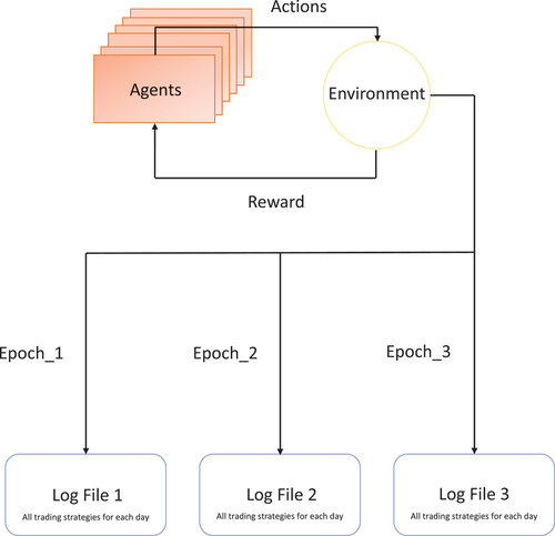
This study developed a DQL-based method to establish an optimal trading strategy for multiple cryptocurrencies. The research process is illustrated in Figure 1. In the proposed method, multiple agents are trained so that they can obtain the maximum reward function, which is the optimal ROI. The reward function is defined in Equation (1)(1) $\mathrm{Reward}\mathrm{function}(\mathrm{ROI})=\left\{\begin{array}{c}\frac{\mathrm{Closing}\mathrm{price}-\mathrm{Opening}\mathrm{price}}{\mathrm{Opening}\mathrm{price}}\mathrm{The}\mathrm{action}\mathrm{is}\mathrm{to}\mathrm{go}\mathrm{long}\\ \frac{\mathrm{Closing}\mathrm{price}-\mathrm{Opening}\mathrm{price}}{\mathrm{Opening}\mathrm{price}}\mathrm{The}\mathrm{action}\mathrm{is}\mathrm{to}\mathrm{go}\mathrm{short}\\ 0\mathrm{The}\mathrm{action}\mathrm{is}\mathrm{to}\mathrm{wait}\mathrm{and}\mathrm{see}\end{array}\right.$(1) . Multiple agents interact with the environment and perform multiple training sessions. During these training sessions, the agents perform different actions, such as go long, go short, and wait and see. These actions are stored in a log file. Finally, the trading strategy that can obtain the maximum reward function (ROI) is selected.

Figure 1. Research procedure.

(1) $\mathrm{Reward}\mathrm{function}(\mathrm{ROI})=\left\{\begin{array}{c}\frac{\mathrm{Closing}\mathrm{price}-\mathrm{Opening}\mathrm{price}}{\mathrm{Opening}\mathrm{price}}\mathrm{The}\mathrm{action}\mathrm{is}\mathrm{to}\mathrm{go}\mathrm{long}\\ \frac{\mathrm{Closing}\mathrm{price}-\mathrm{Opening}\mathrm{price}}{\mathrm{Opening}\mathrm{price}}\mathrm{The}\mathrm{action}\mathrm{is}\mathrm{to}\mathrm{go}\mathrm{short}\\ 0\mathrm{The}\mathrm{action}\mathrm{is}\mathrm{to}\mathrm{wait}\mathrm{and}\mathrm{see}\end{array}\right.$(1)

Agent design

The agents in the proposed method use the bidirectional Q-learning method proposed by Hasselt (2010). This learning method involves using the deep Q-network (DQN) to learn a Q table. The network weights are acquired through the backpropagation of errors during the training stage and then used to update the parameters in the Q table for learning. During the testing stage, the DQN processes the input status and returns the Q value of each action waiting to be performed. Agents perform actions that have the highest Q value. Therefore, the function $R_n\to R_m$ can be derived for an n-dimensional state and m actions. The DQN comprises a target network and an adversarial network, which were proposed by Hasselt (2010) and Wang et al. (2016), respectively. The target network uses Equation (2)(2) $w_{\mathit{t}+1}=w_t-\mathit{\alpha }{\mathrm{\nabla }}_w\in [\left(Q_{w_t}\left(\mathit{x},\mathit{a}\right)-\mathit{Q}\left(\mathit{x},\mathit{a}\right){)}^2\right]$(2) to calculate the target, and the functioning of this network is similar to that of a neural network because its weight $\mathit{w}{ }^{\mathrm{\prime }}$ is equal to the weight $\mathit{w}$ of a neural network. The target network and neural network differ in that the target network copies a new weight from a neural network and does not change its weight until the next update. In DQL, the target and network weight $\mathit{w}$ have a strong correlation. Thus, the predicted Q value and target change during each training phase, which causes instability in the training. Therefore, this study made two changes to the developed DQL-based method to ensure more stable training. First, the DQN was designed to select the optimal action, namely the action with the highest Q value. Second, the target network was used to calculate the target Q value of the action waiting to be taken in the next state.

(2) $w_{\mathit{t}+1}=w_t-\mathit{\alpha }{\mathrm{\nabla }}_w\in [\left(Q_{w_t}\left(\mathit{x},\mathit{a}\right)-\mathit{Q}\left(\mathit{x},\mathit{a}\right){)}^2\right]$(2)

The DQN used in this study included the adversarial network proposed by Wang et al. (2016). This adversarial network calculates $\mathit{D}\left(\mathit{x},\mathit{y},\mathit{a}\right)$ and $\mathit{ma}{x}_b\mathit{Q}\left(\mathit{y},\mathit{b}\right)$ Equation (3)(3) $\mathit{Q}\left(\mathit{x},\mathit{a}\right)={\sum }_y{P}_{\mathit{xy}}\left(\mathit{a}\right)\cdot \left[\mathit{D}\left(\mathit{x},\mathit{y},\mathit{a}\right)+\left({\gamma }^{\mathit{max}}\mathit{Q}\left(\mathit{y},\mathit{b}\right)\right)\right]$(3) , and enable them to be used in the target network. In particular, the adversarial network uses the single fully connected layer of the second-last layer of the DQN, and these layers allow the final aggregation layer to evaluate each value to calculate $\mathit{Q}\left(\mathit{x},\mathit{a}\right)$. To prevent the problem of backpropagation when Equation (3)(3) $\mathit{Q}\left(\mathit{x},\mathit{a}\right)={\sum }_y{P}_{\mathit{xy}}\left(\mathit{a}\right)\cdot \left[\mathit{D}\left(\mathit{x},\mathit{y},\mathit{a}\right)+\left({\gamma }^{\mathit{max}}\mathit{Q}\left(\mathit{y},\mathit{b}\right)\right)\right]$(3) is used for calculation, this study used the aggregation layer to subtract the average $\mathit{ma}{x}_b\mathit{Q}\left(\mathit{y},\mathit{b}\right)$ value of all the possible actions (b) to speed up the training; thus, the reward $\mathit{D}\left(\mathit{x},\mathit{y},\mathit{a}\right)$ could be found without calculating the $\mathit{ma}{x}_b\mathit{Q}\left(\mathit{y},\mathit{b}\right)$ value of each action.

(3) $\mathit{Q}\left(\mathit{x},\mathit{a}\right)={\sum }_y{P}_{\mathit{xy}}\left(\mathit{a}\right)\cdot \left[\mathit{D}\left(\mathit{x},\mathit{y},\mathit{a}\right)+\left({\gamma }^{\mathit{max}}\mathit{Q}\left(\mathit{y},\mathit{b}\right)\right)\right]$(3)

Transaction definition

The agents designed in this study can perform day trades and establish strategies for cryptocurrency trading to obtain the maximum ROI. Because the cryptocurrency market does not actually close, this study defined the closing time of the market as 00:00, after which a new trading day begins. The designed agents had to perform the following actions during each trading day:

1. Go long: Assets are bought and then sold before the market closes.

2. Go short: Assets are sold and then bought before the market closes.

3. Wait and see: Investments are not made on the trading day.

The purpose of the aforementioned transactions is to use the daily price to select an action that maximizes the ROI. If the agents believe that the price will increase during the day, they will go long. By contrast, if they believe that the price will decrease during the day, they will go short. If they do not have sufficient confidence in the market or they believe that the price will remain unchanged, they will wait and see.

The proposed method is based on the aforementioned transactions. This method has the following characteristics. First, multiple agents are trained during different trading periods, which allows each agent to have distinct learning experiences and enables the agents to maximize the ROI in the complex cryptocurrency market. Second, the agents reach a consensus to determine the final trading strategy; each agent uses different decision-making thresholds and parameters to make decisions to go long, go short, or wait and see.

Determining the suitable transaction

When RL is applied to predict cryptocurrency prices, the complexity of the cryptocurrency market must be understood before the actions of agents can be assigned. Therefore, this study trained multiple DQN agents and allocated different types of transactions to these agents to form a trading strategy portfolio to maximize the profits earned in the cryptocurrency market. The DQN agents in the proposed method are as follows:

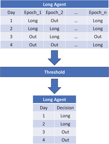
• Go-long agents: Multiple agents are trained at different time intervals and are assigned one action for day trading, namely to go long or to wait and see; these agents are called go-long agents. To execute transactions in the real world, trained go-long agents are used to predict the next action, and the price of the past day is used as the input to create a log file for every agent. The log file includes the action to be performed on each trading day. The go-long agents select the appropriate action from the log file and then use a threshold to determine the final action, as illustrated in Figure 2.

  Figure 2. Q table of go-long agents.

  

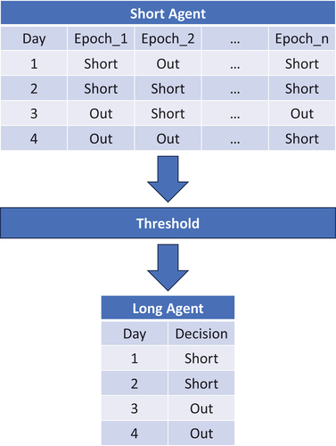
• Go-short agents: The operation of go-short agents is similar to that of go-long agents; however, each go-short agent is assigned to go short or to wait and see. The final action of each go-short agent is also determined by a threshold, as displayed in Figure 3.

  Figure 3. Q table of go-short agents.

  

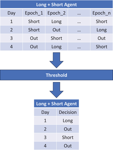
• Go-long + go-short agents: Go-long + go-short agents are assigned to go long or go short. These agents examine the aforementioned two actions to determine a final action, as depicted in Figure 4. These agents perform the wait-and-see action if go-long and go-short agents do not reach a consensus over whether to go long or short or if both go-long and go-short agents suggest to wait and see.

  Figure 4. Q table of go-long and go-short agents.

  

In the proposed method, multiple agents, which consist of different RL classifiers, are trained in the same environment for different time intervals so that they can perform optimal actions. Therefore, the agents can be considered to be investors who perform the same transaction but achieve different investment performance. The agents use a majority vote to determine the optimal transaction. Because the agents have different learning experiences for the environment, they can reduce the uncertainty of the profits earned from the cryptocurrency market. In addition, because the final action of the agents is determined by a majority vote, a certain threshold must be exceeded after the agents reach a consensus to ensure that they opt to go long or short; otherwise, the agents opt to wait and see and not act. The wait-and-see action is used because some scholars have argued that trading every day might not increase the profits of day trading.

Empirical design

Data sets and data splitting

The data sets of this study comprised the 40,354 transaction data of Binance.com from June 1, 2018, to December 31, 2022. The features extracted in this study included the opening price and closing price, which refer to the prices before 00:00:00 Coordinated Universal Time on a trading day and the following day, respectively. This study also extracted the highest price, lowest price, and transaction volume within 24 hr. Transaction volume can assist in the prediction of return. While expanding the sample period to five years reduces the likelihood of environmental changes, for this study we initially planned to use the 10 cryptocurrencies with the highest market capitalization in 2022, but ultimately only selected six cryptocurrencies (BTC, ETH, VET, ADA, TRX, and XRP) because the other four, Avalanche, Solana, Dogecoin, and Terra, had only recently been released. The data cycles of these four cryptocurrencies need to be longer to be more suitable for training Q-learning models.

To help agents learn the different trends in the data collected for the six selected cryptocurrencies, we reviewed these data to identify their uptrends, downtrends, and horizontal trends. For this study, we defined an uptrend, a downtrend, and a horizontal trend as a scenario in which the closing price on the last day of a 1-year cycle was 40% higher than, 40% lower than, and within ± 25% of that on the first day of the cycle, respectively. An analysis of the data revealed that BTC and ETH had an uptrend, VET and TRX had a horizontal trend, and ADA and XRP had a downtrend.

This study used the rolling-window method for data splitting, as presented in Table 1. For BTC and ETH, this study used 578 days of data from June 1, 2018, to December 31, 2019, to train the agents; these data constituted the training samples. Next, we used 365 days of data from January 1 to December 31, 2021 to evaluate the quality of agent training; these data constituted the testing samples. We excluded 366 days of data from January 1 to December 31, 2020 because these data did not reveal an uptrend. For VET and TRX, we used 517 days of data from August 1, 2018 to December 31, 2019 to train the agents. Next, we used 363 days of data from April 1, 2021 to March 31, 2022 to evaluate the quality of agent training. We excluded 456 days of data from January 1, 2020 to March 31, 2021 because these data did not reveal a horizontal trend. For ADA and XRP, we used 517 days of data from August 1, 2018 to December 31, 2019 to train the agents. Next, we used 364 days of data from May 1, 2021 to April 30, 2022 to evaluate the quality of agent training. We excluded 486 days of data from January 1, 2020 to April 30, 2021 because these data did not reveal a downtrend.

Table 1. Periods of the training and testing data sets for the six cryptocurrencies.

Cryptocurrency	Period	Period of the training data	Excluded period	Period of the testing data	Trend
BTC	From to	2018-06-01 2019-12-31	2020-01-01 2020-12-31	2021-01-01 2021-12-31	Uptrend
ETH	From to	2018-06-01 2019-12-31	2020-01-01 2020-12-31	2021-01-01 2021-12-31	Uptrend
VET	From to	2018-08-01 2019-12-31	2020-01-01 2021-03-31	2021-04-01 2022-03-31	Horizontal trend
TRX	From to	2018-08-01 2019-12-31	2020-01-01 2021-03-31	2021-04-01 2022-03-31	Horizontal trend
ADA	From to	2018-08-01 2019-12-31	2020-01-01 2021-04-30	2021-05-01 2022-04-30	Downtrend
XRP	From to	2018-08-01 2019-12-31	2020-01-01 2021-04-30	2021-05-01 2022-04-30	Downtrend

Evaluation indices

Cumulative rate of return

The cumulative rate of return is calculated by dividing the final investment value by the initial investment value and then subtracting 1 from the quotient. The cumulative rate of return reveals the change in the investment value within a specific period.

$\mathrm{Cumulative}\mathrm{rate}\mathrm{of}\mathrm{return}=\left(\frac{\mathrm{Final}\mathrm{investment}\mathrm{value}}{\mathrm{Initial}\mathrm{investment}\mathrm{value}}\right)-1$

Annualized rate of return

In contrast to the cumulative rate of return, the annualized rate of return considers the investment period. The annualized rate of return is calculated as follows:

$\mathrm{Annualized}\mathrm{rate}\mathrm{of}\mathrm{return}={\left(\frac{\mathrm{Final}\mathrm{value}\mathrm{of}\mathrm{the}\mathrm{investment}\mathrm{portfolio}}{\mathrm{Initial}\mathrm{value}\mathrm{of}\mathrm{the}\mathrm{investment}\mathrm{portfolio}}\right)}^{\frac{1}{\mathrm{n}}}-1$

Maximum drawdown

Maximum drawdown (MDD) indicates the downside risk during a time interval. In general, a lower MDD is preferable because it indicates that the investment risk is lower. MDD is calculated as follows (Magdon-Ismail and Atiya 2004):

$\mathit{MDD}=\frac{\left(\mathit{P}-\mathit{L}\right)}{P}$

where P is the peak before the greatest drop and L is the lowest value before the new peak.

Coverage

Coverage (COV) refers to the ratio of the number of decisions made by an agent to go long or short ($\mathit{X}{ }^{\mathrm{\prime }}$) to the total number of decisions made by the agent in the market (X). COV is calculated as follows:

$\mathit{COV}=\frac{\left(\left|\mathit{X}{\mathit{ }}^{\mathrm{\prime }}\right|\right)}{\left|\mathit{X}\right|}$

Empirical results

We used compound interest to calculate the ROI. In addition, we considered actual transactions and included the transaction fee in the ROI calculations. The transaction fee was considered to be 0.075%, as specified by Binance.

Uptrend: BTC

We compared the investment performance of go-short agents, go-long + go-short agents, go-long agents, and the buy-and-hold (B&H) strategy in the BTC market (Table 2). We first trained go-short agents to learn the BTC data and predict BTC transactions from January 1 to December 31, 2021. The empirical results indicated that the annualized rate of return of the go-short agents was 18.55%. The annualized rate of return of these agents was lower than that of the B&H strategy (60.91%) because the number of transactions was 686; therefore, the annual transaction cost for the aforementioned agents was 51.45% under the transaction fee of 0.075%. Because the transaction cost was too high, the profitability achieved by the go-short agents was reduced. However, even if the transaction fee was excluded, the annualized rate of return of the go-short agents was still lower than that of the B&H strategy.

Table 2. Investment performance for BTC.

Strategy	Cumulative rate of return	Annualized rate of return	MDD	COV	The number of transactions	Ranking by rate of return
Go long	84.16%	70.03%	−17.55%	62.26%	52	1
Go long + go short	94.55%	52.28%	−15.71%	52.48%	302	2
Go short	87.97%	18.55%	−16.4%	51.75%	686	4
B&H	–	60.91%	–	–		3

We also trained go-long + go-short agents to learn the BTC data and predict BTC transactions from January 1 to December 31, 2021. The empirical results indicated that the annualized rate of return of the go-long + go-short agents was 52.58%. The annualized rate of return of these agents was higher than that of the go-short agents, but lower than that of the B&H strategy because the number of transactions was 302. Consequently, the annual transaction cost was 22.65%. If the transaction fee was excluded, the annualized rate of return of the go-long + go-short agents was higher than that of the B&H strategy.

Finally, we trained go-long agents to learn the BTC data and predict BTC transactions from January 1 to December 31, 2021. The empirical results indicated that the annualized rate of return of the go-long agents was 70.03%, which was higher than those of the go-long + go-short agents, go-short agents, and of the B&H strategy. This result was caused by the dramatic decrease in the number of transactions for the go-long agents, which considerably reduced the transaction cost. Moreover, the win rate of the go-long agents was higher than that of the other agents and of the B&H strategy.

Uptrend: ETH

We compared the investment performance of go-short agents, go-long + go-short agents, go-long agents, and the B&H strategy in the ETH market (Table 3). We first trained go-short agents to learn the ETH data and predict ETH transactions from January 1 to December 31, 2021. The empirical results indicated that the annualized rate of return of the go-short agents was 197.90%. The annualized rate of return of these agents was lower than that of the B&H strategy (407.18%) because the number of transactions was 348. Therefore, the annual transaction cost for these agents was 26.15% under the transaction fee of 0.075%. Because the transaction cost was too high, the profitability achieved by the aforementioned agents was considerably diminished. However, even if the transaction fee was excluded, the annualized rate of return of the go-short agents was still lower than that of the B&H strategy.

Table 3. Investment performance for ETH.

Strategy	Cumulative rate of return	Annualized rate of return	MDD	COV	The number of transactions	Ranking by rate of return
Go long	240.23%	725.48%	−35.62%	71.26%	86	1
Go long + go short	228.08%	445.57%	−14.66%	62.18%	578	2
Go short	140.75%	197.90%	−14.61%	56.61%	348	4
B&H	–	407.18%	–	–		3

This study also trained go-long + go-short agents to learn the ETH data and predict ETH transactions from January 1 to December 31, 2021. The empirical results indicated that the annualized rate of return of the go-long + go-short agents was 445.57%, which was higher than that of the go-short agents and of the B&H strategy. However, the number of transactions for the go-long + go-short agents was 578; thus, the annual transaction cost was 43.57%.

Finally, we trained go-long agents to learn the ETH data and predict ETH transactions from January 1 to December 31, 2021. The empirical results indicated that the annualized rate of return of the go-long agents was 725.48%, which was higher than that of the go-long + go-short agents, go-short agents, and of the B&H strategy. This result was caused by the dramatic decrease in the number of transactions for the go-long agents, which considerably reduced the transaction cost. Moreover, the COV value of the go-long agents was higher than that of the other agents and of the B&H strategy.

Horizontal trend: VET

We compared the investment performance of go-short agents, go-long + go-short agents, go-long agents, and the B&H strategy in the VET market (Table 4). We first trained go-short agents to learn the VET data and predict VET transactions from April 1, 2021 to March 30, 2022. The empirical results indicated that the annualized rate of return and COV of the go-short agents were − 51.52% and 53.32%, respectively, and the number of transactions for these agents was 526. The annualized rate of return of the go-short agents was lower than that of the B&H strategy (−19.49%).

Table 4. Investment performance for VET.

Strategy	Cumulative rate of return	Annualized rate of return	MDD	COV	The number of transactions	Ranking by rate of return
Go long	83.80%	−14.95%	−41.93%	50.00%	66	1
Go long + go short	1.79%	−28.50%	−20.10%	51.73%	404	3
Go short	72.11%	−51.52%	−34.24%	53.32%	526	4
B&H	–	−19.49%	–	–	–	2

We also trained go-long + go-short agents to learn the VET data and predict VET transactions from April 1, 2021 to March 30, 2022. The empirical results indicated that the annualized rate of return and COV of the go-long + go-short agents were − 28.50% and 51.73%, respectively, and the number of transactions for these agents was 404. The annualized rate of return of the go-long + go-short agents was higher than that of the go-short agents, but lower than that of the B&H strategy.

Finally, this study trained go-long agents to learn the VET data and predict VET transactions from April 1, 2021 to March 30, 2022. The empirical results indicated that the annualized rate of return and COV of the go-long agents were − 14.95% and 50.00%, respectively, and the number of transactions for these agents was 66. The go-long agents had a higher annualized rate of return than did the go-short agents, go-long + go-short agents, and the B&H strategy.

Horizontal trend: TRX

We compared the investment performance of go-short agents, go-long + go-short agents, go-long agents, and the B&H strategy in the TRX market (Table 5). First, we trained go-short agents to learn the TRX data and predict TRX transactions from April 1, 2021 to March 30, 2022. The empirical results indicated that the annualized rate of return and COV of these agents were − 49.32% and 53.18%, respectively, and the number of transactions for these agents was 550. The annualized rate of return of the go-short agents was lower than that of the B&H strategy (−22.19%).

Table 5. Investment performance for TRX.

Strategy	Cumulative rate of return	Annualized rate of return	MDD	COV	The number of transactions	Ranking by rate of return
Go long	−1.16%	−16.95%	−35.50%	50.00%	26	1
Go long + go short	91.59%	−20.98%	−33.35%	51.56%	266	2
Go short	42.31%	−49.32%	−38.09%	53.18%	550	4
B&H	–	−22.19%	–	–	–	3

We also trained go-long + go-short agents to learn the TRX data and predict TRX transactions from April 1, 2021 to March 30, 2022. The empirical results indicated that the annualized rate of return and COV of the go-long + go-short agents were − 20.98% and 51.56%, respectively, and the number of transactions for these agents was 266. The annualized rate of return of the go-long + go-short agents was higher than that of the go-short agents and of the B&H strategy.

Finally, we trained go-long agents to learn the TRX data and predict TRX transactions from April 1, 2021 to March 30, 2022. The empirical results indicated that the annualized rate of return and COV of the go-long agents were − 16.95% and 50.00%, respectively, and the number of transactions for these agents was 26. The go-long agents had a higher annualized rate of return than did the go-short agents, go-long + go-short agents, and the B&H strategy.

Downtrend: ADA

We compared the investment performance of go-short agents, go-long + go-short agents, go-long agents, and the B&H strategy in the ADA market (Table 6). We first trained go-short agents to learn the ADA data and predict ADA transactions from May 1, 2021 to April 30, 2022. The empirical results indicated that the annualized rate of return and COV of the go-short agents were − 11.38% and 48.66%, respectively, and the number of transactions for these agents was 486. The annualized rate of return of the go-short agents was higher than that of the B&H strategy (−40.17%).

Table 6. Investment performance for ADA.

Strategy	Cumulative rate of return	Annualized rate of return	MDD	COV	The number of transactions	Ranking by rate of return
Go long	17.49%	−13.88%	−31.94%	53.85%	64	2
Go long + go short	34.69%	−31.25%	−22.66%	64.36%	390	3
Go short	72.77%	−11.38%	−17.70%	48.66%	486	1
B&H	–	−40.17%	–	–	–	4

We also trained go-long + go-short agents to learn the ADA data and predict ADA transactions from May 1, 2021 to April 30, 2022. The empirical results indicated that the annualized rate of return and COV of the go-long + go-short agents were − 31.25% and 64.36%, respectively, and the number of transactions for these agents was 390. The annualized rate of return of the go-long + go-short agents was lower than that of the go-short agents, but higher than that of the B&H strategy.

Finally, we trained go-long agents to learn the ADA data and predict ADA transactions from May 1, 2021, to April 30, 2022. The empirical results indicated that the annualized rate of return and COV of the go-long agents were − 13.88% and 53.85%, respectively, and the number of transactions for these agents was 64. The annualized rate of return of the go-long agents was higher than that of the go-long + go-short agents and of the B&H strategy, but lower than that of the go-short agents.

Downtrend: XRP

This study compared the investment performance of go-short agents, go-long + go-short agents, go-long agents, and the B&H strategy in the XRP market (Table 7). We first trained go-short agents to learn the XRP data and predict XRP transactions from May 1, 2021 to April 30, 2022. The empirical results indicated that the annualized rate of return and COV of the go-short agents were −36.58% and 54.87%, respectively, and the number of transactions for these agents was 420. The annualized rate of return of the go-short agents was higher than that of the B&H strategy (−60.97%).

Table 7. Investment performance for XRP.

Strategy	Cumulative rate of return	Annualized rate of return	MDD	COV	The number of transactions	Ranking by rate of return
Go long	38.40%	−3.70%	−21.54%	50.00%	76	1
Go long + go short	64.29%	−7.32%	−27.06%	51.08%	230	2
Go short	42.26%	−36.58%	−34.42%	54.87%	420	3
B&H	–	−60.97%	–	–	–	4

This study also trained go-long + go-short agents to learn the XRP data and predict XRP transactions from May 1, 2021, to April 30, 2022. The empirical results indicated that the annualized rate of return and COV of the go-long + go-short agents were −7.32% and 51.08%, respectively, and the number of transactions for these agents was 230. The annualized rate of return of the go-long + go-short agents was higher than that of the go-short agents and B&H strategy.

Finally, we trained go-long agents to learn the XRP data and predict XRP transactions from May 1, 2021 to April 30, 2022. The empirical results indicated that the annualized rate of return and COV of the go-long agents were −3.70% and 50.00%, respectively, and the number of transactions for these agents was 76. The annualized rate of return of the go-long agents was higher than that of the go-short agents, the go-long + go-short agents, and the B&H strategy.

Conclusion and limitations

In this study, we developed a DQL-based method to establish an optimal trading strategy for multiple cryptocurrencies. The developed method uses the same data to train multiple agents so that each agent can learn from the other agents, who have different learning experiences, to improve its prediction of future trends and determine the optimal transaction (go long, go short, or wait and see). The empirical results of this study indicated that the annualized rate of return of go-long agents that learned data was higher than that of the other agents (go-short agents and go-long + go-short agents) and of the B&H strategy for uptrends, horizontal trends, and downtrends. This study also discovered that go-long agents are suitable for a market with an uptrend because they can reduce the risk of trading strategies without affecting the expected profit of investors. Go-long + go-short agents are suitable for executing a stable trading strategy in a market with a downtrend because they can go long or short.

Another limitation of this paper is that overestimating the value of Q is overestimating the value of bias. Many studies have used heuristic extensions and many linear solutions to solve the problem of overestimating the deviation value. In particular, the study of Thrun and Schwartz (1993) pointed out that the overestimation of the Q-value is due to the noise generated by the function approximation. Hasselt’s (2010) study also pointed out that the overestimation is to make the estimate more inclined to be the state of the regional maximum. In addition, van Hasselt, Guez, and Silver (2016) argued that by correcting for the overestimation of Q, the agent is less likely to have separated states, so they applied a multi-step return to reduce the separated states. Multi-step DQN can regulate and reduce divergent behavior and improve training effectiveness. Studies by Hessel et al. (2018) also pointed out that multi-step updating would be more stable under certain conditions than single-step updating. It was also pointed out that multi-step DQN updating is very sensitive to the choice of n-value, which can impact the learning effect if it is not appropriately chosen.

Disclosure statement

No potential conflict of interest was reported by the author(s).

Data availability statement

The datasets generated during and analyzed during the current study are available from the corresponding author upon reasonable request.

Additional information

Funding

This study was supported by the Taiwan Comprehensive University System (TCUS) and the National Science and Technology Council, Taiwan, under [grant NSTC 111-2410-H-019-006-MY3].

References

- Baur, D. G., K. Hong, and A. D. Lee. 2018. Bitcoin: Medium of exchange or speculative assets? Journal of International Financial Markets, Institutions and Money 54:177–22. doi:10.1016/j.intfin.2017.12.004.
- Booth, A., E. Gerding, and F. McGroarty. 2014. Automated trading with performance weighted random forests and seasonality. Expert Systems with Applications 41 (8):3651–61. doi:10.1016/j.eswa.2013.12.009.
- Bouoiyour, J., and R. Selmi. 2015. What does bitcoin look like? Annals of Economics and Finance 16 (2):449–492.
- Bu, S. J., and S. B. Cho. 2018. Learning optimal Q-function using deep Boltzmann machine for reliable trading of cryptocurrency. In Intelligent Data Engineering and Automated Learning–IDEAL 2018, Madrid, Spain, 468–80. Springer International Publishing.
- Chen, C., L. Liu, and N. Zhao. 2020. Fear sentiment, uncertainty, and bitcoin price dynamics: The case of COVID-19. Emerging Markets Finance & Trade 56 (10):2298–309. doi:10.1080/1540496X.2020.1787150.
- Ciaian, P., M. Rajcaniova, and D. A. Kancs. 2016. The economics of BitCoin price formation. Applied Economics 48 (19):1799–815. doi:10.1080/00036846.2015.1109038.
- Corbet, S., A. Meegan, C. Larkin, B. Lucey, and L. Yarovaya. 2018. Exploring the dynamic relationships between cryptocurrencies and other financial assets. Economics Letters 165:28–34. doi:10.1016/j.econlet.2018.01.004.
- Creamer, G., and Y. Freund. 2010. Automated trading with boosting and expert weighting. Quantitative Finance 10 (4):401–20. doi:10.1080/14697680903104113.
- D’Amato, V., S. Levantesi, and G. Piscopo. 2022. Deep learning in predicting cryptocurrency volatility. Physica A: Statistical Mechanics and its Applications 596:127158. doi:10.1016/j.physa.2022.127158.
- Dastgir, S., E. Demir, G. Downing, G. Gozgor, and C. K. M. Lau. 2019. The causal relationship between bitcoin attention and bitcoin returns: Evidence from the copula-based Granger causality test. Finance Research Letters 28:160–64. doi:10.1016/j.frl.2018.04.019.
- Deng, Y., F. Bao, Y. Kong, Z. Ren, and Q. Dai. 2016. Deep direct reinforcement learning for financial signal representation and trading. IEEE Transactions on Neural Networks and Learning Systems 28 (3):653–64. doi:10.1109/TNNLS.2016.2522401.
- Fang, F., C. Ventre, M. Basios, L. Kanthan, D. Martinez-Rego, F. Wu, and L. Li. 2022. Cryptocurrency trading: A comprehensive survey. Financial Innovation 8 (1):1–59. doi:10.1186/s40854-021-00321-6.
- Foley, S., J. R. Karlsen, and T. J. Putniņš. 2019. Sex, drugs, and bitcoin: How much illegal activity is financed through cryptocurrencies? The Review of Financial Studies 32 (5):1798–853. doi:10.1093/rfs/hhz015.
- Gurdgiev, C., and D. O’Loughlin. 2020. Herding and anchoring in cryptocurrency markets: Investor reaction to fear and uncertainty. Journal of Behavioral and Experimental Finance 25:100271. doi:10.1016/j.jbef.2020.100271.
- Hasselt, H. 2010. Double Q-learning. Advances in Neural Information Processing Systems 23:1–9.
- Hessel, M., J. Modayil, H. van Hasselt, T. Schaul, G. Ostrovski, W. Dabney, D. Horgan, B. Piot, M. Azar, and D. Silver. 2018. Rainbow: Combining improvements in deep reinforcement learning. Proceedings of the AAAI Conference on Artificial Intelligence 32 (1). doi:10.1609/aaai.v32i1.11796.
- Hung, C. C., Y. J. Chen, and J. E. Trinidad Segovia. 2021. DPP: Deep predictor for price movement from candlestick charts. PLoS One 16 (6):e0252404. doi:10.1371/journal.pone.0252404.
- Jiang, Z., and J. Liang. 2017. Cryptocurrency portfolio management with deep reinforcement learning. In 2017 Intelligent systems conference, London, UK, 905–13. IEEE.
- Kim, Y. B., J. G. Kim, W. Kim, J. H. Im, T. H. Kim, S. J. Kang, C. H. Kim, and W.-X. Zhou. 2016. Predicting fluctuations in cryptocurrency transactions based on user comments and replies. PLoS One 11 (8):e0161197. doi:10.1371/journal.pone.0161197.
- Kristoufek, L. 2013. BitCoin meets Google trends and Wikipedia: Quantifying the relationship between phenomena of the internet era. Scientific Reports 3 (1):1–7. doi:10.1038/srep03415.
- Kristoufek, L., and E. Scalas. 2015. What are the main drivers of the bitcoin price? Evidence from wavelet coherence analysis. PLoS One 10 (4):e0123923. doi:10.1371/journal.pone.0123923.
- Li, X., and C. A. Wang. 2017. The technology and economic determinants of cryptocurrency exchange rates: The case of bitcoin. Decision Support Systems 95:49–60. doi:10.1016/j.dss.2016.12.001.
- Li, Y., P. Ni, and V. Chang. 2020. Application of deep reinforcement learning in stock trading strategies and stock forecasting. Computing 102 (6):1305–22. doi:10.1007/s00607-019-00773-w.
- Liang, Z., H. Chen, J. Zhu, K. Jiang, and Y. Li. 2018. Adversarial deep reinforcement learning in portfolio management. arXiv preprint arXiv:1808.09940.
- Magdon-Ismail, M., and A. F. Atiya. 2004. Maximum drawdown. The Risk Magazine 17 (10):99–102.
- Nakamoto, S. 2008. Bitcoin: A peer-to-peer electronic cash system.
- Phillips, R. C., D. Gorse, and M. Espinosa. 2018. Cryptocurrency price drivers: Wavelet coherence analysis revisited. PLoS One 13 (4):e0195200. doi:10.1371/journal.pone.0195200.
- Polasik, M., A. I. Piotrowska, T. P. Wisniewski, R. Kotkowski, and G. Lightfoot. 2015. Price fluctuations and the use of bitcoin: An empirical inquiry. International Journal of Electronic Commerce 20 (1):9–49. doi:10.1080/10864415.2016.1061413.
- Pyo, S., and J. Lee. 2020. Do FOMC and macroeconomic announcements affect bitcoin prices? Finance Research Letters 37:101386. doi:10.1016/j.frl.2019.101386.
- Schnaubelt, M. 2022. Deep reinforcement learning for the optimal placement of cryptocurrency limit orders. European Journal of Operational Research 296 (3):993–1006. doi:10.1016/j.ejor.2021.04.050.
- Shavandi, A., and M. Khedmati. 2022. A multi-agent deep reinforcement learning framework for algorithmic trading in financial markets. Expert Systems with Applications 208:118124. doi:10.1016/j.eswa.2022.118124.
- Sovbetov, Y. 2018. Factors influencing cryptocurrency prices: Evidence from bitcoin, ethereum, dash, litcoin, and monero. Journal of Economics and Financial Analysis 2 (2):1–27.
- Stavroyiannis, S., V. Babalos, S. Bekiros, S. Lahmiri, and G. S. Uddin. 2019. The high frequency multifractal properties of bitcoin. Physica A: Statistical Mechanics and its Applications 520:62–71. doi:10.1016/j.physa.2018.12.037.
- Subramanian, H., S. Ramamoorthy, P. Stone, and B. J. Kuipers. 2006. Designing safe, profitable automated stock trading agents using evolutionary algorithms. In Proceedings of the 8th annual conference on Genetic and evolutionary computation, Seattle Washington USA, 1777–84.
- Sutton, R. S., and A. G. Barto. 2018. Reinforcement learning: An introduction. Cambridge, MA: MIT press.
- Thrun, S., and A. Schwartz. 1993. Issues in using function approximation for reinforcement learning. In Proceedings of the 1993 connectionist models summer school, San Mateo, California, 255–63. Psychology Press.
- van Hasselt, H., A. Guez, and D. Silver. 2016. Deep reinforcement learning with double q-learning. Proceedings of the AAAI Conference on Artificial Intelligence 30 (1). doi:10.1609/aaai.v30i1.10295.
- Wang, Z., T. Schaul, M. Hessel, H. Hasselt, M. Lanctot, and N. Freitas. 2016. Dueling network architectures for deep reinforcement learning. In International conference on machine learning, New York, USA, 1995–2003. PMLR.
- Yaga, D., P. Mell, N. Roby, and K. Scarfone. 2019. Blockchain technology overview. arXiv preprint arXiv:1906.11078.
- Yang, H., X. Y. Liu, S. Zhong, and A. Walid. 2020. Deep reinforcement learning for automated stock trading: An ensemble strategy. In Proceedings of the first ACM international conference on AI in finance, New York, USA, 1–8.
- Żbikowski, K. 2015. Using volume weighted support vector machines with walk forward testing and feature selection for the purpose of creating stock trading strategy. Expert Systems with Applications 42 (4):1797–805. doi:10.1016/j.eswa.2014.10.001.