Detecting Changeover Events on Manufacturing Machines with Machine Learning and NC data

ABSTRACT

Changeover events occur in every industrial production when a machine is prepared and setup for production of the next product variant. Changeover times must be acquired with a high degree of validity for product cost calculations, order sequencing, and work schedules. The novelty of this article is a Machine Learning (ML) approach to automatically detect changeover events in production on manufacturing machines without direct human feedback. The machine learning approach uses several algorithms to classify different phases of the changeover process. The changeover of a milling process was defined using different phase concepts (2-phases, 6-phases, 23-phases) to be applicable to other types of manufacturing machines. Different machine learning methods were compared. The best results for the F1 score were achieved with the Random Forest, the CatBoost, and the Extra Trees algorithm (2-phases: 99.4–99.7%, 6-phases: 85.2–85.9%, 23-phases: 77.7–79.4%). It is shown that detecting changeover events can be realized based on data from an NC of a manufacturing machine without data from external sensors (2-phases: 98.9%, F1 score).

Introduction

Today, digitization is an important element in increasing the efficiency of industrial production. In the transformation to a smart factory, logistic and production processes must be equipped with sensors and data processing. Ideally, factories or production lines can be planned from scratch, incorporating all the latest technology (greenfield approach). In contrast, existing production facilities, referred to as brownfield, are often equipped with old machines without additional sensors or network functionalities (Strauß et al. 2018). Accordingly, processes and IT systems have grown organically and are heterogeneous. The implementation of digitization techniques is correspondingly complex (Forstner and Dümmler 2014). Therefore, the research project Optimization of Processes and Machine Tools through Provision, Analysis and Target/Actual Compar- ison of Production Data (OBerA) was established to support metalworking companies from the region of northern Bavaria in digitizing their system landscape.

During the research project, it was worked out with the project partners that especially the changeover times cannot be measured reliably in practice. The approach to measuring these times presented in this article is based on machine control data and anonymous personal data from the work system in which the changeover is conducted. It does not require manual feedback from the employee nor data from additional external sensors. Due to the efforts of time recording and analysis, estimates for times are often used (Ringsquandl, Lamparter, and Lepratti 2015). With the presented approach, time data can be determined automatically and efficiently for all occurring changeover situations and free of operating errors and estimation inaccuracies.

Section 1.1 describes the application and challenges of changeover times in industry, and discusses the novelty of the approach. In Section 1.2, existing research work is presented and a research question is derived. Section 1.3 introduces the structure of the article.

Problem statement

Changeovers between manufacturing orders occur frequently on an industrial shop floor. They are necessary to set up the working environment for a new product type. During the changeover process, only sample products are manufactured to confirm that the process setup for the upcoming new product type is correct and the manufacturing process can be conducted in a capable way. Changeovers are consequently regarded as production loss (Gelders and Van Wassenhove 1982), and the reduction of changeover times has been a crucial task for manufacturing operations and is addressed by popular Lean Management methods like Single Minute Exchange of Die (SMED) (Mali and Inamdar 2012).

As changeover events occur at the beginning of a manufacturing order, they influence the overall throughput time of the order. Therefore, changeover times are considered in production planning and scheduling (Wolsey 1997), and they are an important part of the company’s industrial time data basis. Handling changeover times belongs to the responsibilities of industrial engineering departments, which are usually professionalized in recording time data by analyzing the activities of operators during the changeover process.

In industrial engineering, time data can be differentiated into actual and planned times. Planned time stands for “the planned duration of a specific time period” and is the intended duration of an operation resulting from a planning process in industrial engineering. The actual time is the realized duration of an operation, which “may be less than, equal to, or greater than corresponding planned time” (ISO 22400–2:2014E 2014).

There are numerous possibilities and methods to determine planned times for defined processes such as changeovers, e.g. surveys, estimates, self-recordings, multi-moment recordings, and calculations. In addition, there are methods with predefined times and process modules or time data determination with the help of time recordings and measurements (Lotter, Deuse, and Lotter 2016, 196). The choice of a suitable method for determining planned times depends on the required accuracy of the time data. For example, when planned times are applied for payment or product cost calculations, time data can be less accurate than when used for capacity planning or scheduling (Sihn et al. 2016, 373).

While there exist several methods for the determination of planned times, numerous difficulties arise with the recording of actual times. A measurement of actual times usually takes place at the workplace, either through a direct time recording conducted by the industrial engineering with the operator, or times are reported by the operator through time protocols or entered directly into IT systems (Lotter, Deuse, and Lotter 2016, 196). In the OBerA research project, the following main causes for heterogeneous actual changeover times were identified:

• Standardizing the content of a changeover process is difficult. In practice, too precise definitions require a high amount of subsequent maintenance when changes are made; definitions that are too general lead to high deviations in the feedback of time data to the Enterprise Resource Planning (ERP) system.

• Employees or groups of employees (e.g. fixed shift staffing) disregard changeover standards and work according to standards they have set themselves.

• Employees do not report changeover activities promptly but collectively at the end of the shift or forget to report them.

• Employees report back incorrectly, incompletely, or the target times instead of actual times.

• Reporting across shifts is not organized or not possible from an IT point of view.

Through an automatic determination of actual changeover times, a major gain in efficiency and validity can be achieved. Statistical analyses of past changeover times can be used to generate reliable target times. These target times can be utilized for an established time management system or for (semi-) automated synchronization of time data into ERP systems.

In current ERP systems such as SAP, data structures for so-called changeover matrices are already available (SAP n.a., 2024a (accessed 17.06.2024)). A changeover matrix contains the changeover times for all theoretically possible changeover processes within a product range ($n^2-\mathit{n}$ combinations). Statistically secure manual data collection for complete changeover matrices of a product portfolio is time consuming. For a product range with 50 products at 30 repetitions 73,500 changeover times per machine type have to be determined. If changeover matrices are available, they can already be used in current ERP systems, e.g. for optimizing the production order sequence (SAP n.a., 2024b (accessed 17.06.2024)). This research project, therefore, offers the possibility of filling changeover matrix data structures automatically in ERP systems and making ERP-side optimization approaches more reliable and automated due to a higher precision of the input data.

The innovation of the approach is, first of all, that industrial engineering departments no longer have to spend time recording the changeover times, as a Machine Learning (ML) system derives the changeover times from existing data of the work system. Another innovation of the presented approach is the possibility to identify sub-changeover phases, i.e. information on specific changeover processes and when they are being carried out (e.g. setting up a tool or workpiece). This automatic recognition of changeover phases can also be statistically evaluated and used for the overall optimization of the changeover processes, e.g. in work preparation with methods like SMED.

Literature review

Machine learning techniques are already frequently used in industrial manufacturing. Song and Luo (2022) identify four main fields of application in particular:

• Scheduling (for planning and controlling the production operations as well as resource allocation),

• Monitoring (for deviation reaction management and decision support),

• Quality (for quality control and defect detection),

• Fault detection (for equipment fault information and machine maintenance).

For the special case of manufacturing in production lines, Kang, Catal, and Tekinerdogan (2020) also add to this enumeration the “reduction of waste” and the “increase in yield” as fields of application for machine learning.

A large number of different manufacturing processes exist for industrial production. Especially manufacturing processes with a defined cutting-edge play an important role. Within these processes, milling and turning processes are considered to be the dominant subgroup (König and Klocke 2002).

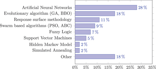
For manufacturing processes, Du Preez and Oosthuizen (2019) have specifically investigated the application of machine learning techniques. Figure 1 shows that machine learning techniques are used particularly frequently in turning and milling with its related process of drilling and boring. Figure 2 shows that Artificial Neural Networks are applied particularly frequently, followed by evolutionary algorithms and response surface methodology.

Figure 1. ML applications in manufacturing (aggregated from Du Preez and Oosthuizen (2019)).

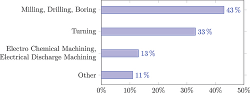
Figure 2. ML techniques in manufacturing (aggregated from Du Preez and Oosthuizen (2019), ABC: artificial bee colony, BBO: biogeography based optimization algorithm, GA: genetical algorithms, PSO: particle swarm optimization).

In addition to the application fields of quality, process, and condition monitoring mentioned above, Denkena et al. (2021) also point to the optimization of manufacturing process parameters, e.g. cutting depth/width, cutting speed, and feed rate as a field of application for machine learning in production. The authors also address the potential of machine learning in the production order-related view of manufacturing processes. For production management and production controlling, machine learning methods can be used in particular to predict time components of the planned throughput and delivery time as well as to detect deviations between actual and planned scheduling parameters. Though not explicitly mentioned in Denkena et al. (2021), changeover times are an essential time component in manufacturing which influences the potential application possibilities.

Overall, ML methods have not been used to detect changeover times in an industrial manufacturing environment. Comparable objectives are described in the following research articles: In (Ringsquandl, Lamparter, and Lepratti 2015), process times, in general, are estimated using a least-squares linear regression model to detect changes in contexts in a specific use case situation. In (Zeberli et al. 2021), the authors use Principal Component Analysis (PCA) to detect failures in changeover operations of biopharmaceutical drug product manufacturing. Similarly, in (Quatrini et al. 2020), an anomaly detection and process phase classification based on Random Forests and Decision Trees in a pharmaceutical use case is presented. The authors of (Ayvaz and Alpay 2021) propose the ML methods Random Forest and XGBoost to detect production stops to facilitate predictive maintenance in a manufacturing environment. In (Can and Heavey 2016), an approach is shown to estimate processing times, i.e. cycle times based on Manufacturing Execution System (MES) data by applying a genetic algorithm.

None of the mentioned approaches realizes an automatic detection of changeover times with ML. In addition, the applications of these approaches are generally not located in an industrial manufacturing environment. None of the approaches has the goal of building a detailed historical changeover time data base for synchronization with an ERP system (see Section 1.1).

In previous research, the authors showed that it is generally feasible to detect phases of the changeover process with a large set of external sensors attached to a milling machine. The ML models achieved an F1 score of 96% for a balanced Random Forest and 97% for a Random Forest model (Engelmann et al. 2020; Miller et al. 2021).

Overall, implementation efforts for a large set of external sensors are assumed to be too high for broad industrial use on many manufacturing machines. It also became apparent that the models still had the potential for optimization in terms of accuracy, especially for detecting sub-phases of the changeover process. The challenge for the research work of this article was to detect changeover using data directly from the Numerical Control (NC) of the manufacturing machine instead of a large set of external sensors. In addition, the quality of the models shall be improved. This approach would also generate the possibility to use and retrain the ML models directly on the NC of a machine and embed many NCs into a federated learning context (Khajehali et al. 2023).

This paper attempts to answer the following overarching research question: “Is it possible to determine the changeover status of a manufacturing machine by a classification approach with machine learning based on NC data without manual feedback from the human machine operator?.”

Article structure

The underlying methodology of this article is the CRISP-DM phase model for conducting data mining projects. It was initially created based on the experiences of practitioners from the field of data mining (Chapman et al. 2000). Over the years, it became a frequently used de-facto standard for data mining projects (Schröer, Kruse, and Gómez 2021) and was also adjusted to the demands of specific knowledge domains, i.e. engineering applications (Huber et al. 2019).

Figure 3 shows the structure of the article as a flow chart. The specific CRISP-DM phases are mentioned in parentheses:

Figure 3. Structured approach.

• Section 1 contains a general introduction to the research task and provides information about the industrial use case. (Business understanding phase)

• The data structure, sources, and acquisition process are described in Sections 2.1, 2.2, and 2.3. (Data understanding phase)

• Section 2.4 explains the data preparation and the labeling process. In Section 3.1, the feature selection is discussed, and the chosen set of features is then evaluated by the PCA and t-Distributed Stochastic Neighbor Embedding (t-SNE) methods in Section 3.2. (Data preparation phase)

• The chosen ML algorithms are explained in Section 3.3. Section 3.4 comments on the sizes of the test and training set. (Modeling phase)

• Section 4 defines the performance metrics and presents the results of these metrics applied to the different trained models (Evaluation phase).

The article closes with a discussion (Section 5), conclusions (Section 6.1), and a suggestion for further research (Section 6.2). The CRISP-DM deployment phase is not included in this article. It contains the steps of transferring the trained model to the organization’s IT systems, connecting the model to production data services, and monitoring the model performance (Chapman et al. 2000).

Material

In this section, the different phases of the changeover process for milling are explained (Section 2.1), and the used milling machine is introduced (Section 2.2). Finally, the concept for the data acquisition (Section 2.3) as well as the data preparation and labeling is described (Section 2.4).

Phases of the changeover process

While setting up a machine, several manual activities are conducted by the machine operator. The content and sequence of operations depend on the type of machine tool which is set up. In the OBerA project, the research was focused on milling processes.

Based on previous research by the authors, three different phase concepts were defined to model the milling process (see also Appendix A):

• 2-phase approach (No. 1: Changeover including intermittent idle time, No. 2: Production phase)

• 6-phase approach (No. 1: Starting phase, No. 2: Main phase, No. 3: Ending phase, No. 4: Idle/break phase, No. 5: Production phase, No. 6: Quality control phase) and

• 23-phase approach (No.: 1–19 Sub phases, No. 20: Idle/break phase, No. 21: Production phase, No. 22: General quality control, No. 23: Work-piece quality control).

For a distinction between changeover and production, two phases (2-phase approach) would have been sufficient, but for optimizing activities in production engineering, more phases are preferable. Based on the assumption that more phases complicate the classification with ML, an intermediate phase concept with six phases (6-phase approach) and a detailed phase concept with 23 phases (23-phase approach) were defined. All phase approaches are summarized in Table A1.

To realize an automatic detection of the defined changeover phases, an ML classification approach is described in Section 3. To train ML models, changeover processes under real production conditions need to be supervised, and labels for the specific phases need to be assigned to sensor measurements and their timestamps (see Section 2.4). Based on specific states of the machine/operator environment, different phases of the changeover shall be detected. For this multi-class classification problem, suited ML algorithms need to be selected (see Section 3.3).

Milling machine tool

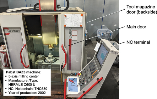
Figure 4 shows the HERMLE C600 U milling machine that was used for this research. The machine has 5-axis kinematics and an NC HEIDENHAIN iTNC 530, which is suitable for the HEIDENHAIN DNC interface. The HERMLE machine was located on an industrial shop floor at the company Pabst from the OBerA project consortium. Additionally, the machine was equipped with a Wago IoT-Box 9466, which measures the machine’s power consumption with Rogowski coils. The machine was used for standard manufacturing orders in a multi-shift environment.

Figure 4. Milling machine HERMLE C600 U at the company pabst.

Data acquisition

The NC was connected to a NUC mini PC via an Ethernet switch. Additionally, the Wago IoT-Box for power measurements was connected via LAN and sent data through Message Queuing Telemetry Transport (MQTT) to a message broker hosted on the PC. The data was then processed by the graphical programming environment Node-RED and sent to a Structured Query Language (SQL) database. Communication between an agent on the PC and the NC was achieved with the HEIDENHAIN DNC interface. The data was sent from the agent via the MQTT protocol to the Cybus Connectware hosted on a Virtual Machine (VM). The Connectware also had a Node-RED adaptation where the data was processed and sent to the same SQL database. Data over a period of two working days (day 1 with approx. 5.5 h and day 2 containing approx. 6.75 h of data with 20,829 rows of data in total) was used for the training of the ML models.

In this research, two changeover sessions were used. The original dataset recording contained 13 sessions (Engelmann and Schmitt 2024). For labeling sessions 3 to 12, information from the worker terminals was used instead of timestamps from process-intermittent monitoring. The timestamps from the worker terminal needed to be omitted as their frequency of 5 minutes was too inaccurate to receive reliable ML models (Schmitt and Engelmann 2024).

Data preparation and labeling

Preprocessing the data is one of the main tasks in ML projects (Wirth and Hipp 2000). The data from the NC and from the external sensor setup was written into a SQL database. For each data channel, a record with the measured value as well as a description and the corresponding timestamp was added to the database every two seconds. To evaluate the data with a machine learning model in Python, a dataframe was created by adding the recorded feature values to timestamps.

The resulting table based on timestamps showed gaps since not all measured values were available for every timestamp. To fill gaps, the last valid value was used or, in the case of the spindle override, the feed override, and the feed rate of the machine, the moving average over the last 4 values, for the speed of the main spindle, a moving average over the last 2 values was used. A one-class SVM was used to detect outliers and 1,111 data points were removed. The dataframe was then labeled with the data from the changeover recording. During data recording of the changeover process, the defined individual phases of all three phase concepts were identified together with a machine operator and documented with their timestamps. Then the dataset with the sensor data and the changeover recording were merged using the timestamp information. Therefore, three columns with the changeover phases described in Section 2.1 were added to the dataset. Therefore, each row of the dataset contains the timestamp, the values for the ten selected features, and the three labels for the 2-phases, the 6-phases, and the 23-phase approach. For modeling, the feature values have to be standardized. Therefore, the Z-transformation was applied using the Python scikit-learn StandardScaler method.

Methods

This section explains the methodological approach to create ML models for changeover detection. Section 3.1 describes the sensor and feature selection. In Section 3.2 the feature set is evaluated. Afterward, the list of chosen ML algorithms is presented (Section 3.3). Section 3.4 explains the sizes of the test and training datasets.

Sensor and feature selection

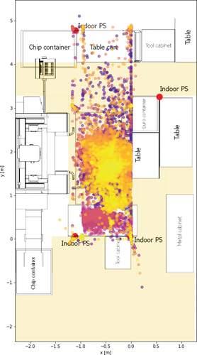
For the training of the ML models, several NC-external and NC-provided sensors were available. As an NC-external sensor, an indoor Positioning System (PS) was established to monitor the operator’s walking path during the changeover (Neuber et al. 2022). An exemplary position recording of a changeover process is shown in Appendix B. In addition, Rogowski coils for measuring the machine power consumption were used (see Section 2.2).

All sensors that were directly connected to the NC and provided by the NC data interface were regarded here as NC-provided sensors. For the HERMLE machine, possible features could also be found in the circuit plans, e.g. door switches 2001. These features were available as variables by the Cybus Connectware interface that used the HEIDENHAIN DNC interface to export these internal variables (see Section 2.3). Additionally, the NC provided data that was generated by the NC itself e.g. the current DNC mode. The specific NC-generated datasets were regarded here also as “data channels.” All data channels were provided by the Cybus Connectware interface. In total, the NC of the HERMLE machine offers more than 400 potential features. From this selection, a team of experts chose 19 sensors and data channels.

Table 1 shows the initial selection of the sensors with a total of 22 sensors and data channels (NC-external: 3, NC-internal: 19). This selection needed to be refined during the next feature selection steps: Rough feature selection, Fine feature selection, and Performance-based feature set refinement.

Table 1. Sensor and data channel selection.

Sensors	Initial Selection
NC-external	IndoorPS (x, y)
	PowerConsumption
NC-provided	CabinDoorLocks (side, front)
	ChipCleaningGunStatus
	CoolantFlow status
	DNCMode
	DoorStatuses (Main, Tooling)
	DriveStatus
	FeedRate
	OverrideFeed
	OverrideSpindle
	PocketTable
	ProgramChange
	ProgramDetail
	RapidTraverseKey
	SpindleApproval
	SpindleCleaning
	SpindleSpeed
	ToolNumber

Rough feature selection

For the rough feature selection, data from the 22 sensors and data channels was recorded. Because data is recorded, it is necessary to use the word “feature” in the following sections instead of sensors and data channels. The word “features” is synonymous with “attributes,” which in turn are defined as “properties of things” (Drummond 2017). Sensors and data channels deliver measured values for these properties. Feature extraction (here: feature selection), is defined to be the process of “determining which attributes are necessary for learning” (Drummond 2017).

To achieve a reduction in the number of pre-selected sensors and data channels, the recorded data points for all 22 sensors and data channels were analyzed using basic statistical methods. An analysis of the minimum/maximum values and the standard deviation showed that in 3 cases, there were no changes in the values during the observation period (CabinDoorLockSide, SpindleApproval, and OverrideSpindle). These features were removed from the dataset because the minimum value was equal to the maximum value and the standard deviation was zero. It was assumed that these features had no information value (see Figure C1 in Appendix C). The total of 22 features was reduced to 19.

Fine feature selection

In the next step, a correlation analysis was conducted. It was based on a linear correlation coefficient, which is able to show redundancy among features (Yu and Liu 2003). The limit value $\mathit{r}$ for the Pearson correlation coefficient was chosen to be $\mathit{r}=|65\mathrm{\%}|$, which corresponds to a medium to strong correlation (Hagl 2007).

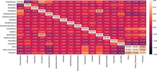
Accordingly, 4 features were removed by searching the heatmap for correlation coefficient entries above $65\mathrm{\%}$ and below $-65\mathrm{\%}$ and evaluating the related features. The corresponding correlation heatmap for the 19 features can be found in Figure F1 in Appendix F:

• The parameter for changes to the ProgramDetail was removed as it appeared to be very highly linked to the ProgramStatus.

• In the same way, the CoolantFlow was found to be strongly correlated with the SpindleSpeed, the PowerConsumption of the machine, and the DriveStatus. The feature was, therefore, removed from the dataset.

• Then the PowerConsumption was removed as it was correlated to SpindleSpeed and DriveStatus.

• Finally, DoorStatusMain was removed because it is medium to highly correlated with DriveStatus.

In the end, a heatmap with 15 remaining features was generated (see Figure 5). From this heatmap, 4 features can be identified, which have a very small range of correlation coefficients:

Figure 5. Final correlation heatmap for 15 features.

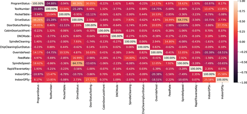
• ChipCleaningGunStatus: $[-0.62\mathrm{\%},0.88\mathrm{\%}]$

• CabinDoorLockFront: $[-1.64\mathrm{\%},1.32\mathrm{\%}]$

• DNCMode: $[-3.77\mathrm{\%},3.18\mathrm{\%}]$

• RapidTraverseKey: $[-5.21\mathrm{\%},2.35\mathrm{\%}]$

The features that were not removed were kept for the subsequent stage of the analysis. Upon closer inspection, these specific features displayed rare status changes within a dataset of 21,940 rows. The frequency of status changes for each feature was as follows: 1 for ChipCleaningGunStatus, 5 for CabinDoorLockFront, 22 for DNCMode, and 54 for RapidTraverseKey.

In the last step of the feature refinement, all features were checked for their individual importance for preliminary classification models. For this purpose, the method of Permutation Feature Importance (PFI) is explained and applied in the next section.

Performance-based feature set refinement

As shown in the previous section, after correlation analysis, irrelevant features might remain in the selection. Such irrelevant features have a negative impact on the necessary computing power and even on the performance of a model. Furthermore, they can impair the interpretability of the results (Miao and Niu 2016). The method of “Model Reliance” or also PFI which was described by (Breiman 2001; Fisher, Rudin, and Dominici 2019) for Random Forests, and (Molnar 2019, 154) shall be applied in this last step of feature selection (here: feature refinement). The detailed procedure of conducting a PFI analysis is explained in Appendix D.

For the remaining 15 features, a Random Forest was trained according to the described procedure in the appendix. After permuting the columns, the features were ranked by importance (see Table 2). It was possible to remove five more features from the selection (RapidTraverseKey, ChipCleaningGunStatus, SpindleCleaning, DNCMode, and CabinDoorLockFront).

Table 2. Reduced number of model features by PFI.

Selection	Weight	Feature
Included	$0.2549\pm 0.0107$	OverrideFeed
	$0.1186\pm 0.0071$	ToolNumber
	$0.1181\pm 0.0092$	IndoorGPSy
	$0.0683\pm 0.0047$	IndoorGPSx
	$0.0639\pm 0.0046$	PocketTable
	$0.0579\pm 0.0056$	SpindleSpeed
	$0.0548\pm 0.0055$	ProgramStatus
	$0.0524\pm 0.0070$	DriveStatus
	$0.0313\pm 0.0019$	DoorStatusTooling
	$0.0108\pm 0.0023$	FeedRate
Excluded	$0.0009\pm 0.0000$	RapidTraverseKey
	$0\pm 0.0000$	ChipCleaningGunStatus
	$0\pm 0.0000$	SpindleCleaning
	$0\pm 0.0000$	DNCMode
	$0\pm 0.0000$	CabinDoorLockFront

ChipCleaningGunStatus, SpindleCleaning, DNCMode, and CabinDoorLockFront showed a weight of $0\pm 0.0000$ and were therefore excluded. RapidTraverseKey was also excluded as the weight of $0.0009\pm 0.0000$ is factor 12 lower than the FeedRate with $0.0108\pm 0.0023$. All of these features except SpindleCleaning were already identified in the previous chapter as candidates for removal. With the results from PFI they could be excluded more reliably. Therefore, the selection of sensors and data channels could finally be reduced from 15 to 10 (indoor positioning x and y, door status tooling, drive status, feed rate, override feed, pocket table, program status, spindle speed, tool number).

Evaluation of the independent variables

In the following, the data is visualized using PCA (Abdi and Williams 2010) to gain insights into the intrinsic dimensionality of the data. PCA is a dimensionality reduction as well as an exploratory data analysis method, which projects a dataset on the eigenvectors of its covariance matrix $\mathit{S}$ corresponding to the largest eigenvalues of $\mathit{S}$. This leads to a separation on the axis with the highest variance (Géron 2019, p. 219).

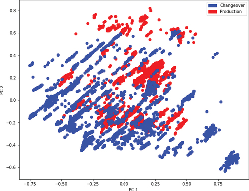
Figure 6 shows the data separated into two classes, namely changeover (blue) and production (red). The data was projected via PCA from 10 features down to two features (PC1 and PC2). Although the data was not completely linearly separable, at some points in time the PCA still managed to separate the data. However, PCA is only able to separate the data if features are linearly correlated (Lever, Krzywinski, and Altman 2017) and thus can perform a linear projection. To overcome the limitations of the PCA a non-linear embedding technique was applied to the data.

Figure 6. Data projected on the eigenvectors corresponding to the largest eigenvalues via principal component analysis (PCA).

In Figure 7 t-Distributed Stochastic Neighbor Embedding (t-SNE) (Van der Maaten and Hinton 2008) has been applied with different parameters. t-SNE is a non-linear embedding technique, which aims to reduce the dimensionality of the data. This is done by preserving the distances of close data points during the embedding. Global distances are meaningless in t-SNE, thus similar data points grouped together can also occur close to other clusters of originally far away data points.

Figure 7. Data embedded into two dimensions via t-Distributed Stochastic Neighbor Embedding (t-SNE) using perplexity values between 20 and 50. Blue points represent the production phase and red points the changeover phase.

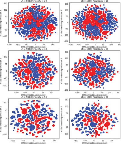
An important parameter in t-SNE is the perplexity. The perplexity is related to the number of nearest neighbors that are used in other manifold learning algorithms (Van der Maaten and Hinton 2008). It is recommended to use a maximum perplexity of 50. This recommendation is followed and a perplexity range between 20 and 50 with learning rates of 500 and 1.000 was applied.

Due to the large dataset size, smaller perplexity parameters led to a non-differentiable data cloud. The visualizations show that the data is mainly differentiable using non-linear techniques. Furthermore, the results are interpreted under the time characteristics of the dataset. The plots then indicate that at almost all time steps the phases are clearly distinguishable in low dimensions, which results in clusters of the same labels. Only for a few data points more information is needed to distinguish the classes, which then results in single outliers in another label’s data cloud.

Selection of machine learning algorithms

In (Miller et al. 2021) it was shown, that Decision Trees, Support Vector Machines (SVM), Neural Networks, and (balanced) Random Forest algorithms are suited for the underlying classification task (see also Section 2.1). In this article, additionally, gradient-boosted trees were selected for the training of the machine learning models.

As a baseline architecture for the Neural Network, a classical sequential Multi-Layer Perceptron (MLP) was considered, as proposed in (Wang, Yan, and Oates 2017). The basic layer structure was adapted from (Rustam et al. 2020). Details about the layer structure and the most important hyperparameters can be found in Table 3 and Appendix E.

Table 3. Algorithm selection.

Algorithm category		Selected ML algorithms
Decision Trees		Decision Tree
Ensemble methods	Forests of randomized trees	Random Forest
		Balanced Random Forest
		Extra Trees
	Gradient boosted trees	Catboost
		LightGBM
		XGBoost
Neural Network	Layer structure	Input (10)
		Dense (300, Sigmoid/Tanh)
		Batch Normalization
		Dropout (0.2/0.3)
		Dense (40/50, Linear/Relu)
		Batch Normalization
		Dense (2/6/23, Softmax)
	Hyperparameters	Nadam optimizer (0.01/0.05),
		epochs (90/120),
		batch size (32/64)
SVM		SVM (RBF kernel)
		regularization parameter
		C=1e6

CatBoost, LightGBM, and XGBoost are based on gradient boosting and offer improvements to other ensemble methods in terms of training speed and generalization capability. It is also reported that these algorithms show very good performances when Random Forest algorithms perform comparably well (Bentéjac, Csörgö, and Martínez-Muñoz 2021).

The Random Forest algorithm was the best-performing algorithm in the previous research activities. Hence, another Random Forest-like technique was added to the choice of algorithms, the so-called Extremely Randomized Tree (ERT) (Geurts, Ernst, and Wehenkel 2006). ERT or Extra Trees work similarly to Random Forests, except for the random choice of cut points, which leads to faster computation time. Additionally, Extra Trees uses real samples instead of bootstrap samples to reduce variance. So, the mentioned three gradient boosting and the Extra Tree algorithms were included in this research approach (see Table 3).

The hyperparameters of all selected algorithms were optimized using the randomized search algorithm, which is a further development of the frequently used grid search technique for hyperparameters (Géron 2019, 78). It offers better performances when especially small sets of hyperparameters are tuned (Liashchynskyi and Liashchynskyi 2019). For improvement in metrics and detailed hyperparameters of the applied algorithms, see Appendix G and the available and documented source code (link available in 6.2).

Test and training datasets

The next step was to divide the data into training and test sets. 80% were used to train the algorithms and the remaining 20% for testing. For Neural Networks, the training set was subdivided to obtain a validation set of 10% of the total dataset. This was necessary as no validation set is defined in the algorithm.

Evaluation of results

This section evaluates the application of the different ML algorithms on the recorded data. Section 4.1 explains the utilized performance metrics to evaluate the results. In Section 4.2, these metrics are applied and discussed. In Section 4.3, the final modeling step is explained.

Performance metrics

A popular metric to evaluate ML models is the F1 score. The value range of the F1 score is between 0 and 1. If it is 0, none of the data points were correctly assigned to the corresponding class. If the F1 score equals 1, all values were correctly assigned to the class (Sokolova, Japkowicz, and Szpakowicz 2006, 430).

For the use with imbalanced datasets, which are discussed in the paper of Chicco and Jurman (Chicco and Jurman 2020, 10), as well as in Akosa’s work (Akosa 2017), the Matthews Correlation Coefficient (MCC) is preferred. MCC has the same range as the F1 score, from 0 to 1. In this paper, for better visual representation, the ranges of the F1 score and the MCC were converted into the corresponding percentage values with 0 as 0% and 1 as 100%.

Phases are imbalanced when the quantity of data points is distributed differently in the phases to be classified. Figures 8 and Figure 9 show the occurrences of the phases in the different phase concepts. Figure 8 shows that phases 13, 20, and 21 (Running and optimizing the NC program, Idle/break, and Production) are more frequent than the other phases.

Figure 8. Occurrences 23-phases.

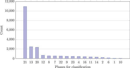
Figure 9. Occurrences in 6-phases.

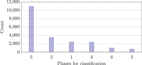
Figure 9 shows that phase 5 (Production), groups 1, 2, 4 (Start, Main, Idle/break), and groups 3, and 6 (End, Quality) are very differently distributed. For the 2-phases concept, the occurrences are more equally distributed, with 10,939 occurrences for the production phase and 9,890 occurrences for the changeover phase. Due to the overall imbalanced character of the data, the MCC shall also be used in this research for model evaluation along with the F1 score.

Comparison of the results

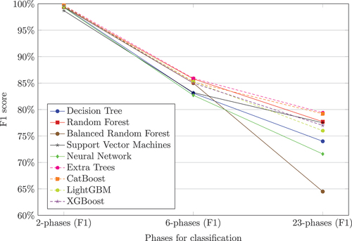
Figure 10 shows the F1 performance of the different hyperparameter-optimized ML algorithms. For the 2-phase approach, all algorithms achieved an F1 score of 98.7% to 99.7%. Extra Trees and CatBoost performed best with a 99.7% F1 score, followed by the XGBoost with 99.6%. The Balanced Random Forest showed the strongest decrease in performance of all algorithms for the 23-phase approach but is still competitive in the 6-phase approach. The Neural Network performed comparably weakly in the 6-phase and 23-phase approaches. The algorithms Extra Trees (79.4%), CatBoost (79.2%), and Random Forest (77.7%) showed the best performance for the 23-phase approach.

Figure 10. Comparison of F1 scores.

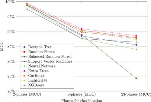
Figure 11 shows the MCC performances. In comparison to Figure 10, all the algorithms showed very good performances of 98.8% − 99.5% for the 2-phase approach except SVM with 97.5%. The performance loss over the 6-phase and 23-phase approach was much smaller when applying the MCC for performance evaluation, e.g. for 23-phase the Balanced Random Forest achieved 74.3% MCC instead of the corresponding 64.5% F1 score. Neural Networks again performed weakly, achieving the lowest MCC for the 6-phase approach (87.6%) and the second worst result for the 23-phase approach (84.0%). The best performances were shown by the algorithms Extra Trees (2: 99.4%, 6: 90.9%, 23: 88.6%), CatBoost (2-phases: 99.3%, 6-phases: 89.7%, 23-phases: 88.3%), and Random Forest (2: 98.9%, 6: 90.4%, 23: 87.9%).

Figure 11. Comparison of MCC values.

Overall, it turned out that the F1 score and MCC differ in the way that the achieved performance values for the MCC were slightly higher than the F1 score across the 6- and 23-phase classification approaches. For the underlying dataset, which is highly imbalanced, MCC was the more reliable performance measure. No algorithm was capable of keeping a consistent performance over all-phase concepts, and all algorithms decreased in performance as more phases were classified. The Random Forest algorithm and the boosting algorithms CatBoost, LightGBM, and XGBoost, as well as the Extra Trees, showed the best performances.

Final modeling

The feature selection showed that only the indoor PS was needed from the external sensors. The PowerConsumption, measured with the Rogowski coils, was eliminated during the feature selection process, as described in Section 3.1.2.

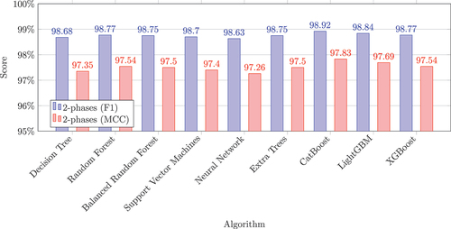
For the classification of two phases, an F1 score of 98.7% to 99.7% and an MCC of 98.8% − 99.5% except SVM with 97.5% was achieved (see Section 4.2). Figure 12 shows the results of training the ML algorithms without the indoor PS. Performance results of 97.26% − 97.83% MCC and 98.63% − 98.92% F1 score are achieved without revisiting the feature selection process. This result was based exclusively on the NC data without any external sensors.

Figure 12. Comparison F1 score and MCC value for the final modeling of two phases.

Discussion

The models presented in this article are trained for a particular machine. When adapting the models to other machines, several limitations must be considered. Engelmann et al. (2024) describe that data retrieval may be impeded for certain machine types due to the lack of support for necessary protocols by the machine controllers. In such cases, data can be obtained from external sensors. Furthermore, the transition from this brownfield approach to a greenfield approach was investigated. It is important to note that different features may be accessible from external sensors compared to internal sensors. Additionally, the features available for the models may vary depending on the manufacturers of the controllers.

The changeover detection concept from this article is currently being transferred to another 5-axis milling machine equipped with a Siemens 840D SL NC. Several features described in Section 3.1 are also available, including the main door status, feed override, and spindle speed. Additional features such as the feed rate and power consumption can be monitored for all five axes, the spindle, and the tool change system, resulting in an increased number of features for the models. Preliminary results indicate that the detection performance for the 2-phase approach is comparable to the findings presented in Section 4.2 (see also Section 6.2).

For adaption to other machines, the 6-phase and 23-phase approaches need to be revisited to ensure that the changeover process is consistent across the considered machines. Nonetheless, the general methodology described in this paper can be applied to different machines.

Table 4 shows the features selected in Section 3.1.3. Since the feature set was trained in a supervised learning approach, it is essential to consider the impact of changing operating conditions on the machine learning model (Neuber et al. 2022) investigated the influence of fluctuation on an indoor positioning system within a production environment. The findings indicate that the position of the worker is strongly influenced by structural objects on the shop floor, such as tool trolleys, material pallets, or partition walls. Standardization can be achieved through precise layout planning of the production with zones. However, fluctuations caused by the presence or absence of objects like material pallets can be incorporated into the model’s training data (Biju, Schmitt, and Engelmann 2024). The investigations in Section 4.4 also show that the position features can be removed from the feature set for model creation, resulting in only a slight decrease in model performance metrics.

Table 4. Influence on a ML model by operation conditions.

Feature	Influenced by	Controlled by
IndoorGPSy	Human workflow	Leave out
IndoorGPSx	Human workflow	Leave out
OverrideFeed	Human workflow	Standardization of workflow
DoorStatusTooling	Human workflow	Standardization of workflow
ProgramStatus	Human workflow	Standardization of workflow
DriveStatus	Human workflow	Standardization of workflow
FeedRate	Machining process	Standardization of machining
SpindleSpeed	Machining process	Standardization of machining
ToolNumber	Machining process	Standardization of machining
PocketTable	Machining process	Standardization of machining

The features OverrideFeed, DoorStatusTooling, ProgramStatus, DriveStatus depend on how the human operator executes the workflow. To ensure that operators consistently perform work sequences, Lean Management employs standardized work practices to reduce deviations in the work sequences (Torres, Pimentel, and Duarte 2020).

The features FeedRate, SpindleSpeed, and PocketTable result from the machining process planning. With the exception of small batch production, these parameters are usually determined by the process development department and are specified for stable machining operation to achieve consistent product quality for different material batches. The transfer of machining parameters directly into the NC of a machine can be regarded as an established procedure in industry (Zhang, Yongxian, and Bai 2010).

Conclusions and further research

In this section, the conclusions are derived (Section 6.1), and an outlook for further research is given (Section 6.2).

Conclusions

In Section 4.3, it was shown that the trained models reached high MCC and F1 scores without external sensors (F1: $>$98.63%, MCC: $>$97.26%). After PowerConsumption was excluded during feature selection, the optimized models were good enough so that excluding the external indoor PS reduced the high MCC and F1 scores only 2% slightly (F1: 0.07% − 0.78%, MCC: 1.54% − 1.67%). For a shop floor environment, this is the most preferable situation. Workers do not need to carry a positioning tag for the changeover detection and all data could be acquired directly from the NC. In conclusion, this feature setup shows the feasibility of an approach that relies only on NC-provided data without external sensors.

Referring to the initial research question in Section 1.2, it can be concluded that it is possible to determine the changeover status of a manufacturing machine by a classification approach with ML without external sensors. However, it must be noted that the detection of the changeover showed the best results only for the 2-phase approach. Here, the identified algorithms could reliably detect the start and stop of changeovers. This high reliability is important when changeover times are synchronized with ERP systems and applied, e.g. in product calculations or order sequencing. For classical engineering optimizations of changeovers, it would be beneficial to distinguish between more changeover processes more accurately.

The results of the shown approach showed that the selected machine learning algorithms performed worse the more phases were classified. One explanation could be the duration of the production phase, which is long compared to the other phases. This is evident in the imbalanced data in each phase for the 6-phase approach and especially for the 23-phase approach. The proportion between changeover and production time can have different reasons. It can be caused by the character of the production, i.e. for large-scale production, the share of changeover time in the total production time is small, while for single-item and small-scale production, the share is significantly higher. A larger proportion of changeover time can also originate in a lack of engineering activities on the shop floor, i.e. missing changeover optimizations (Focke and Steinbeck 2018, 50).

From the results, it can also be seen that the Balanced Random Forest and Neural Networks performed weaker than the other ML algorithms in the presented use case. These algorithms were optimized with standard optimization techniques. Therefore, the results should not be generalized and concluded that these algorithms are not suited at all for multi-class problems. Specifically for Neural Networks, there exist further optimization approaches, intensive ablation studies (Meyes et al. 2019). The intention of this article was to compare different ML algorithms that were improved with standard optimizations. Nevertheless, the results also indicate that, in practice, algorithms show different robustness with multi-class tasks when applied to imbalanced data.

Further research

In order to be able to generalize the results shown, further data of milling operations from different machines must be recorded. For further research an experiment for 5-axis milling with 30 changeover sequences applying three different products is prepared. The publication of the modeling and the data set along with a dataset descriptor is planned for the end of 2024.

As human operators are conducting working sequences such as changeover processes, deviations such as changing the sequence or skipping steps can naturally occur, even if standardized work principles are applied (Section 4). Process deviations can be desirable as they contain also process improvement possibilities (Team 2002, 22). Therefore the modeling approach should be robust enough to handle sequence deviations. When suited data is used in the training process, the presented approach to classify feature variables at a specific point in time may be better suited to handle deviations, than a time series classification approach with a specific window size. This needs to be analyzed and compared in further research.

The created models must then be applied to this data and analyzed if there is also an effect of imbalanced data. Special attention must be paid to the data amount within the individual phases (2-phases, 6-phases, and 23-phases). Furthermore, it needs to be analyzed if the identified 23 phases can be generalized for the milling process. It is also necessary to investigate in detail the effect of the detection accuracy of the start and end times of the changeover operations. Here, it is of particular interest how inaccuracies in the determined time data affect application use cases, e.g. in product costing or order sequencing.

In this research, Neural Networks performed weaker than other ML algorithms. In this article, discrete states were used for the classification of the phases. However, there exist specific approaches based on Neural Networks like Fully Convolutional Neural Networks (FCN), Residual Networks (ResNet), and Multi-scale Convolutional Neural Networks (MCNN) to achieve a classification of longer time periods, i.e. time-series (Wang, Yan, and Oates 2017; Yan et al. 2021). Also, graph-based approaches for sequences of discrete states can be considered (Zhou et al. 2020). In particular, Neural Networks for time series will be evaluated in further research.

CRediT authorship contribution statement

Bastian Engelmann: Conceptualization, Methodology, Validation, Formal analysis, Investigation, Resources, Writing – original draft, Writing – review and editing, Visualization, Supervision, Project administration, Funding acquisition. Anna-Maria Schmitt: Conceptualization, Methodology, Software, Validation, Formal analysis, Investigation, Data curation, Writing – original draft, Writing – review and editing, Visualization. Moritz Heusinger: Software, Validation, Investigation, Writing – original draft, Writing – review and editing. Vladyslav Borysenko: Software, Validation, Writing – original draft, Writing – review and editing, Visualization. Niklas Niedner: Methodology, Software, Investigation, Data curation, Writing – original draft. Jan Schmitt: Formal analysis, Writing – review and editing.

Nomenclature/Notation

ERP	=	Enterprise Resource Planning
ERT	=	Extremely Randomized Tree
MCC	=	Matthews Correlation Coefficient
MES	=	Manufacturing Execution System
ML	=	Machine Learning
MQTT	=	Message Queuing Telemetry Transport
MLP	=	Multi-Layer Perceptron
NC	=	Numerical Control
OBerA	=	Optimization of Processes and Machine Tools through Provision, Analysis and Target/Actual Comparison of Production Data
PCA	=	Principal Component Analysis
PS	=	Positioning System
PFI	=	Permutation Feature Importance
SMED	=	Single Minute Exchange of Die
SQL	=	Structured Query Language
SVM	=	Support Vector Machines
t-SNE	=	t-Distributed Stochastic Neighbor Embedding
VM	=	Virtual Machine

Acknowledgements

The authors gratefully thank Pabst Komponentenfertigung GmbH and Cybus GmbH for their contribution to the research.

Disclosure statement

No potential conflict of interest was reported by the author(s).

Data availability statement

The Python source code and the dataset are available under: https://github.com/SuperAms/Detecting_Changeover.

Supplemental material

Supplemental data for this article can be accessed online at https://doi.org/10.1080/08839514.2024.2381317

Additional information

Funding

This work was supported by the state of Bavaria (Bayerisches Staatsministerium für Wirtschaft, Landesentwicklung und Energie) under [Grant no. IUK 530/010].

Appendix A.

Different changeover phases

Table A1. Different changeover phases, updated from (Miller et al. 2021).

6-phases	23-phases	Description
Start	1	Reporting changeover start at the terminal
	2	Machine table cleaning
	3	Remove fixture from the machine table
	4	Component fastening to fixture
	5	Move fixture to the machine table
	6	Attach fixture to the machine table
	7	NC program loading
	8	Tool presetting
	9	Tool magazine filling and tool control
	10	Enter tool dimensions
Main	11	Insert/remove tool directly into/from spindle
	12	Zero point setting
	13	NC program optimizing and running
End	14* + 15	Component cleaning and dismantling
	16* + 17	Component deburring and remeasuring
	18**	Upload the optimized NC program
	19**	Reporting changeover stop at the terminal
Idle/break	20	Idle/break
Production	21	Production
Quality	22	General quality control
	23	Work-piece quality control

* only first number used for labeling. ** not used in this research.

Appendix B.

Indoor Positioning System

Figure B1 shows the different positions of an operator which were tracked by an indoor positioning system of the company Localino (https://localino.net/).

Figure B1. Position data.

Appendix C.

Statistical Information

The information from descriptive statistics of each sensor is detailed in Table C1.

Table C1. Statistical information of each sensor.

	mean	std	min	25%	50%	75%	max
DoorStatusTooling	0.039	0.194	0	0	0	0	1
DriveStatus	0.542	0.498	0	0	1	1	1
FeedRate	607.645	3269.364	−32590	0	0	310	32732
IndoorGPSx	−0.483	0.288	−1.416	−0.702	−0.486	−0.27	0.22
IndoorGPSy	1.451	0.948	−1.103	0.622	1.51	1.914	5.104
OverrideFeed	85.175	33.112	0	84	100	100	150
PocketTable	4.699	7.231	0	0	1	8	30
ProgramStatus	1.439	1.635	0	0	2	2	6
SpindleSpeed	1828.053	2594.748	0	0	0	4599	10046
ToolNumber	11.023	8.434	0	8	8	19	32
CabinDoorLockFront	0	0.015	0	0	0	0	1
ChipCleaningGunStatus	1	0.007	0	1	1	1	1
DNCMode	0.001	0.032	0	0	0	0	1
RapidTraverseKey	0.002	0.050	0	0	0	0	1
SpindleCleaning	0.007	0.086	0	0	0	0	1
CoolantFlow	0.316	0.465	0	0	0	1	1
DoorStatusMain	0.328	0.469	0	0	0	1	1
PowerConsumption	2529.934	2060.587	−17186.1	930.78	2078.47	3586.23	28956
ProgramDetail	1.438	1.613	0	0	2	2	6
CabinDoorLockSide	0	0	0	0	0	0	0
OverrideSpindle	100	0	100	100	100	100	100
SpindleApproval	0	0	0	0	0	0	0

Appendix D.

Permutation Feature Importance (PFI)

The PFI can be calculated according to the steps shown in Figure D1:

Figure D1. Permutation feature importance (PFI) approach.

In the first step of the procedure, a classification model $\mathit{f}$ is trained with the original dataset, and the model error $e_{\mathit{orig}}$ is calculated (S1). The mean squared error is a suitable error function $\mathit{L}$. The classification model $\mathit{f}$ can be generated by different algorithms e.g. Neural Networks or Random Forest algorithms. In the next step, a new feature matrix $X_{\mathit{perm}}$ is generated from the feature matrix $\mathit{X}$ by permuting the entries of a feature $X_j$ (S2). The matrix $X_{\mathit{perm}}$ contains a feature that has no relationship with the target vector $\mathit{y}$. In step 3 (S3) of the permutation procedure, the new model error $e_{\mathit{perm}}$ is calculated. If the model error $e_{\mathit{perm}}$ increases in comparison to $e_{\mathit{orig}}$, it can be assumed that the feature is highly relevant to the model. However, if the model error changes only slightly or even decreases, the feature is unimportant for model creation. In step 4 (S4), the feature importance $\mathit{F}{I}_j$ is determined. It corresponds to the difference of the model error after the permutation $e_{\mathit{perm}}$ to the initial model error $e_{\mathit{orig}}$. The feature importance $\mathit{F}{I}_j$ is stored in a list $\mathit{p}$ (S5). This procedure is repeated until each feature from the initial dataset has been permuted once. Then the entries of the list $\mathit{p}$ are sorted in descending order (S6). A ranking of the importance of all features is received in this way.

Appendix E.

Neural Network Architecture

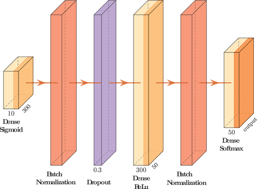
The Neural Network was implemented in TensorFlow Keras. The final Neural Network hyperparameters were found using randomized search. The architecture for the 2- and 23- phase approach is shown in Figure E1. The first layer is a Dense layer (yellow) with 10 input features and 300 neurons and Tanh as an activation function. This is followed by a Batch Normalization and a Dropout layer (30%, purple) to prevent overfitting. The next layer is a second Dense layer with 50 neurons and ReLu as activation function followed by a second Batch Normalization layer. At the end is a Dense layer with 2 or 23 neurons for the different approaches and the Softmax activation function.

Figure E1. Neural network architecture for the 2 and 23-phase approaches.

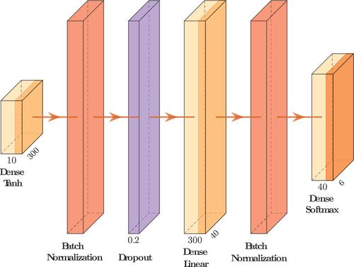
The Neural Network for the 6-phase approach has a similar structure (see Figure E2). The differences are the activation function for the first Dense layer (sigmoid) the dropout rate (20%) and the second Dense layer with 40 neurons and a linear activation function. The final Dense layer has 6 neurons.

Figure E2. Neural network architecture for the 6-phase approach.

The Nadam optimizer was used for all phase approaches with different learning rates (2-phases: 0.01, 6-phases: 0.01, 23-phases: 0.05). For the 2-phase approach, a batch size of 64 and 120 epochs were used. The 6- and 23-phase approaches had 90 epochs and a batch size of 32 and 64 respectively. Furthermore, the sparse categorical cross-entropy function was used as the loss function.

Appendix F.

Correlation Heatmap

The correlation heatmap for the 19 recorded features is shown in Figure F1.

Figure F1. Correlation heatmap for 19 features.

Appendix G.

Hyperparameter Tuning

The values for the F1 score and MCC after hyperparameter tuning are detailed in Table G1. The original F1 score and MCC were subtracted from the tuned values. Therefore, positive differences indicate an increase in performance. The asterisk indicates that the classification results with optimization equaled the original results. The standard parameters turned out to be already optimal.

Table G1. Differences between optimized and non-optimized hyperparameters. The asterisk represents no changes in hyperparameters.

	2-phases		6-phases		23-phases
Algorithm	F1 [%]	MCC [%]	F1 [%]	MCC [%]	F1 [%]	MCC [%]
Neural Network	0.45	0.89	3.96	2.54	8.04	3.86
SVC	$\ast$	$\ast$	$\ast$	$\ast$	$\ast$	$\ast$
Decision Tree	$\ast$	$\ast$	$\ast$	$\ast$	$\ast$	$\ast$
Balanced Random Forest	$\ast$	$\ast$	0.13	0.03	2.12	−0.40
Random Forest	$\ast$	$\ast$	$\ast$	$\ast$	$\ast$	$\ast$
Extra Trees	$\ast$	$\ast$	$\ast$	$\ast$	$\ast$	$\ast$
Catboost	0.12	0.24	$\ast$	$\ast$	1.04	0.66
LightGBM	$\ast$	$\ast$	$\ast$	$\ast$	0.80	0.07
XGBoost	$\ast$	$\ast$	$\ast$	$\ast$	$\ast$	$\ast$

References

- Abdi, H., and L. Williams. 2010. Principal component analysis. Wiley Interdisciplinary Reviews: Computational Statistics 2 (4):433–37. doi:10.1002/wics.101.
- Akosa, J. 2017. Predictive accuracy: A misleading performance measure for highly imbalanced data. Proceedings of the SAS Global Forum 12:1–4. Cary, NC, USA: SAS Institute Inc.
- Ayvaz, S., and K. Alpay. 2021. Predictive maintenance system for production lines in manufacturing: A machine learning approach using IoT data in real-time. Expert Systems with Applications 173:114598. doi:10.1016/j.eswa.2021.114598.
- Bentéjac, C., A. Csörgö, and G. Martínez-Muñoz. 2021. A comparative analysis of gradient boosting algorithms. Artificial Intelligence Review 54 (3):1937–67. doi:10.1007/s10462-020-09896-5.
- Biju, V. G., A.-M. Schmitt, and B. Engelmann. 2024. Assessing the influence of sensor-induced noise on machine-learning-based changeover detection in CNC machines. Sensors 24 (2):330. doi:10.3390/s24020330.
- Breiman, L. 2001. Random forests. Machine Learning 45 (1):5–32. doi:10.1023/A:1010933404324.
- Can, B., and C. Heavey. 2016. A demonstration of machine learning for explicit functions for cycle time prediction using MES data. 2016 Winter Simulation Conference (WSC), 11-14 December 2016, Washington, DC, USA, 2500–11.
- Chapman, P., J. Clinton, R. Kerber, T. Khabaza, T. Reinartz, C. Shearer, R. Wirth. 2000. CRISP-DM 1.0: Step-by-step data mining guide. SPSS Inc 9:13.
- Chicco, D., and G. Jurman. 2020. The advantages of the Matthews correlation coefficient (MCC) over F1 score and accuracy in binary classification evaluation. BMC Genomics 21 (1):1–13. doi:10.1186/s12864-019-6413-7.
- Denkena, B., M.-A. Dittrich, H. Noske, K. Kramer, and M. Schmidt. 2021. Anwendungen des maschinellen Lernens in der Produktion aus Auftrags- und Produktsicht. Zeitschrift Für Wirtschaftlichen Fabrikbetrieb 116 (5):358–62. Accessed june 13, 2024. doi:10.1515/zwf-2021-0068.
- Drummond, C. 2017. Attribute. In Encyclopedia of machine learning and data mining, ed. C. Sammut and G. I. Webb, 73–75. Boston, MA: Springer US.
- Du Preez, A., and G. A. Oosthuizen. 2019. Machine learning in cutting processes as enabler for smart sustainable manufacturing. Procedia Manufacturing 33:810–17. doi:10.1016/j.promfg.2019.04.102.
- Engelmann, B., and A.-M. Schmitt. March, 2024. Series production data set for 5-axis CNC milling. Data 9 (5):66. doi:10.3390/s24020330.
- Engelmann, B., A.-M. Schmitt, L. Theilacker, and J. Schmitt. 2024. Implications from legacy device environments on the conceptional design of machine learning models in manufacturing. Journal of Manufacturing and Materials Processing 8 (1):15. doi:10.3390/jmmp8010015.
- Engelmann, B., S. Schmitt, E. Miller, V. Bräutigam, and J. Schmitt. 2020. Advances in machine learning detecting changeover processes in cyber physical production systems. Journal of Manufacturing and Materials Processing 4 (4):108. doi:10.3390/jmmp4040108.
- Fisher, A., C. Rudin, and F. Dominici. 2019. All models are wrong, but many are useful: Learning a Variable’s importance by studying an entire class of prediction models simultaneously. Journal of Machine Learning Research 20 (177):1–81.
- Focke, M., and J. Steinbeck. 2018. Steigerung der Anlagenproduktivität durch OEE-Management. Wiesbaden: Springer Gäbler.
- Forstner, L., and M. Dümmler. 2014. Integrierte Wertschöpfungsnetzwerke–Chancen und Potenziale durch Industrie 4.0. e & i Elektrotechnik und Informationstechnik 131 (7):199–201. doi:10.1007/s00502-014-0224-y.
- Gelders, L. F., and L. N. Van Wassenhove. 1982. Hierarchical integration in production planning: Theory and practice. Journal of Operations Management 3 (1):27–35. doi:10.1016/0272-6963(82)90019-5.
- Géron, A. 2019. Hands-on machine learning with Scikit-learn, Keras, and TensorFlow: Concepts, tools, and techniques to build intelligent systems. Sebastopol, CA: O’Reilly Media, Inc.
- Geurts, P., D. Ernst, and L. Wehenkel. 2006. Extremely randomized trees. Machine Learning 63 (1):3–42. doi:10.1007/s10994-006-6226-1.
- Hagl, S. 2007. Schnelleinstieg Statistik. Haufe Praxisratgeber. Freiburg: Haufe-Lexware GmbH & Co. KG.
- Huber, S., H. Wiemer, D. Schneider, and S. Ihlenfeldt. 2019. DMME: Data mining methodology for engineering applications – a holistic extension to the CRISP-DM model. Procedia CIRP, 12th CIRP Conference on Intelligent Computation in Manufacturing Engineering 79:403–08. Gulf of Naples, Italy. Accessed July 18–20, 2018. doi:10.1016/j.procir.2019.02.106.
- ISO 22400-2:2014(E). 2014. Automation systems and integration — key performance indicators (KPIs) for manufacturing operations management — part 2: Definitions and descriptions. Standard. Geneva, CH: International Organization for Standardization.
- Kang, Z., C. Catal, and B. Tekinerdogan. 2020. Machine learning applications in production lines: A systematic literature review. Computers & Industrial Engineering 149:106773. doi:10.1016/j.cie.2020.106773.
- Khajehali, N., J. Yan, Y.-W. Chow, and M. Fahmideh. 2023. A comprehensive overview of IoT-based federated learning: Focusing on client selection methods. Sensors 23 (16):7235. doi:10.3390/s23167235.
- König, W., and F. Klocke. 2002. Einleitung, 1–2. Berlin, Heidelberg: Springer Berlin Heidelberg. doi:10.1007/978-3-662-07202-8_1.
- Lever, J., M. Krzywinski, and N. S. Altman. 2017. Points of significance: Principal component analysis. Nature Methods 14 (7):641–42. doi:10.1038/nmeth.4346.
- Liashchynskyi, P., and P. Liashchynskyi. 2019. Grid search, random search, genetic algorithm: a big comparison for NAS. CoRR Abs/1912.06059. doi:10.48550/arXiv.1912.06059.
- Lotter, B., J. Deuse, and E. Lotter. 2016. Die Primäre Produktion. Berlin, Heidelberg: Springer Berlin Heidelberg 10:978–3. doi:10.1007/978-3-662-53212-6.
- Mali, Y. R., and K. H. Inamdar. 2012. Changeover time reduction using SMED technique of lean manufacturing. International Journal of Engineering Research and Applications 2 (3):2441–45.
- Meyes, R., M. Lu, C. W. de Puiseau, and T. Meisen. 2019. Ablation studies in artificial neural networks. arXiv preprint arXiv:1901.08644.
- Miao, J., and L. Niu. 2016. A survey on feature selection. Procedia Computer Science 91 (4):919–26. doi:10.1016/j.procs.2016.07.111.
- Miller, E., V. Borysenko, M. Heusinger, N. Niedner, B. Engelmann, and J. Schmitt. 2021. Enhanced changeover detection in industry 4.0 environments with machine learning. Sensors 21 (17):5896. doi:10.3390/s21175896.
- Molnar, C. 2019. Interpretable machine learning. Victoria, British Columbia, Canada: Leanpub.
- Neuber, T., A.-M. Schmitt, B. Engelmann, and J. Schmitt. 2022. Evaluation of the influence of machine tools on the accuracy of indoor positioning systems. Sensors 22 (24):10015. doi:10.3390/s222410015.
- Quatrini, E., F. Costantino, G. Di Gravio, and R. Patriarca. 2020. Machine learning for anomaly detection and process phase classification to improve safety and maintenance activities. Journal of Manufacturing Systems 56:117–32. doi:10.1016/j.jmsy.2020.05.013.
- Ringsquandl, M., S. Lamparter, and R. Lepratti. 2015. Estimating processing times within context-aware manufacturing systems. IFAC-Papersonline 48 (3):2009–14. 15th IFAC Symposium onInformation Control Problems inManufacturing. doi:10.1016/j.ifacol.2015.06.383.
- Rustam, F., A. Ahmad Reshi, I. Ashraf, A. Mehmood, S. Ullah, D. Muhammad Khan, and G. Sang Choi. 2020. Sensor-based human activity recognition using deep stacked multilayered perceptron model. Institute of Electrical and Electronics Engineers Access 8:218898–910. doi:10.1109/ACCESS.2020.3041822.
- SAP. n.a. June 17, 2024a. Campaign optimization. https://help.sap.com/doc/saphelp_snc70/7.0/en-US/cd/2a673b19f27654e10000000a114084/content.htm.
- SAP. n.a. June 17, 2024b. Setup matrix. https://help.sap.com/doc/saphelp_scm700_ehp02/7.0.2/en-US/8e/4ec95360267614e10000000a174cb4/frameset.htm.
- Schmitt, A.-M., and B. Engelmann. 2024. A series production data set for five-axis CNC milling. Data 9 (5):66. https://www.mdpi.com/2306-5729/9/5/66. doi:10.3390/data9050066.
- Schröer, C., F. Kruse, and J. M. Gómez. 2021. A systematic literature review on applying CRISP-DM process model. Procedia Computer Science 181:526–34. doi:10.1016/j.procs.2021.01.199.
- Senn, M., and HERMLE 300.91K4-0.3. 2001. Schaltplan. Industriestr.8-12, 78559 Gosheim: HERMLE.
- Sihn, W., A. Sunk, T. Nemeth, P. Kuhlang, and K. Matyas. 2016. Produktion und Qualität: Organisation, Management, Prozesse. München: Carl Hanser Verlag GmbH Co KG.
- Sokolova, M., N. Japkowicz, and S. Szpakowicz. 2006. Beyond accuracy, F-score and ROC: A family of discriminant measures for performance evaluation. Australasian joint conference on artificial intelligence, December 4-8, Hobart, 1015–21. Springer.
- Song, Z., and S. Luo. 2022. Application of machine learning and data mining in manufacturing industry. Frontiers in Computing and Intelligent Systems 2 (1):47–53. doi:10.54097/fcis.v2i1.2966.
- Strauß, P., M. Schmitz, R. Wöstmann, and J. Deuse. 2018. Enabling of predictive maintenance in the brownfield through low-cost sensors, an IIoT-architecture and machine learning. 2018 IEEE International conference on big data (big data), December 10-13, Seattle, WA, USA, 1474–83. IEEE.
- Team, P. P. D. 2002. Standard work for the shopfloor. The Shopfloor Series. Taylor & Francis. https://books.google.de/books?id=ye7gwAEACAAJ.
- Torres, D., C. Pimentel, and S. Duarte. 2020. Shop floor management system in the context of smart manufacturing: A case study. International Journal of Lean Six Sigma 11 (5):823–48. doi:10.1108/IJLSS-12-2017-0151.
- Van der Maaten, L., and G. Hinton. 2008. Visualizing data using t-SNE. Journal of Machine Learning Research 9 (11):2579–2605
- Wang, Z., W. Yan, and T. Oates. 2017. Time series classification from scratch with deep neural networks: A strong baseline. 2017 International joint conference on neural networks (IJCNN), May 14-19, Anchorage, AK, USA, 1578–85. IEEE.
- Wirth, R., and J. Hipp. 2000. CRISP-DM: Towards a standard process model for data mining. Proceedings of the 4th international conference on the practical applications of knowledge discovery and data mining 1:29–40. Manchester.
- Wolsey, L. A. 1997. MIP modelling of changeovers in production planning and scheduling problems. European Journal of Operational Research 99 (1):154–65. doi:10.1016/S0377-2217(97)89646-4.
- Yan, R., A. Julius, M. Chang, A. Fokoue, T. Ma, and R. Uceda-Sosa. 2021. STONE: Signal temporal logic neural network for time series classification. 2021 International Conference on Data Mining Workshops (ICDMW), December 07-10, Auckland, New Zealand, 778–87. IEEE.
- Yu, L., and H. Liu. 2003. Feature selection for high-dimensional data: A fast correlation-based filter solution. Proceedings of the 20th international conference on machine learning (ICML-03), August 21-24, Washington, DC, USA, 856–63.
- Zeberli, A., S. Badr, C. Siegmund, M. Mattern, and H. Sugiyama. 2021. Data-driven anomaly detection and diagnostics for changeover processes in biopharmaceutical drug product manufacturing. Chemical Engineering Research & Design 167:53–62. doi:10.1016/j.cherd.2020.12.018.
- Zhang, Y., L. Yongxian, and X. Bai. 2010. The research on the intelligent Interpreter for ISO 14649 programs. In Advances in computation and intelligence, ed. Z. Cai, C. Hu, Z. Kang, and Y. Liu, 523–34. Berlin, Heidelberg: Springer Berlin Heidelberg.
- Zhou, J., G. Cui, S. Hu, Z. Zhang, C. Yang, Z. Liu, L. Wang, C. Li, and M. Sun. 2020. Graph neural networks: A review of methods and applications. AI Open 1:57–81. doi:10.1016/j.aiopen.2021.01.001.