Use of Socio-economic, Climatic, and Land use Land Cover Patterns in Solid Waste Forecasting with Integrated Gradient LSTNet Based Model in Lomé, Togo

ABSTRACT

Few studies have explored recurrent neural network models in municipal solid waste (MSW) generation forecasting regarding the inefficiency of conventional and probabilistic tools. This study aimed to develop a new approach of Integrated Gradient Long- and Short-term Time series Network (LSTNet+IG)-based models, assess the baseline neural network models, and provide features influences explanation on MSW generation by using socio-economic, climatic, and Land Use Land Cover (LULC) patterns. Hence, the Random Forest Regressor and Gradient Boosting Regressor methods were used for feature selection, and the IG component was incorporated to LSTNet model for feature influence explanation alongside baseline models implementation. Moreover, the metrics such as root relative square error (RSE) and relative absolute error (RAE) were used to evaluate models’ performance. As a result, the LSTNet+IG outperforms others with the lowest RSE (0.9727) and RAE (0.9108). Moreover, five key influencing features were found, namely the number of households and institutions, mean relative humidity, electricity consumption, built area, and mean temperature. Hence, the socio-economic, climatic, and LULC features in MSW generation forecasting have shown to be important in decision-making for effective MSW management. Therefore, the LSTNet+IG model adoption by stakeholders could help to anticipate and mitigate MSW mismanagement through better planning.

Introduction

Municipal solid waste (MSW) generation forecasting over decades has gained particular attention in research studies around the world to improve waste management. Several methods have been developed and are known under the terms of descriptive statistics (DS), regression analysis (RA), material flow (MF), time series analysis (TSA), and artificial intelligence (AI). The DS method uses population growth and average per capita waste generation as main predictors (Ali Abdoli et al. 2012) and is known to not be effective for MSW generation forecasting owing to the dynamic phenomena related to the MSW management system (Abbasi and Abduli 2013). For its simplicity based on mathematics and well-known statistics theory, RA is used by researchers to forecast MSW generation (Abbasi and El Hanandeh 2016). It relies on assumptions of independence, constant variance, and normality of errors on input features and has limitations on forecasting MSW generation in real-world problems (Hockett, Lober, and Pilgrim 1995). Moreover, MF method depicts the dynamic properties but is used to only forecast the total MSW generation, not MSW collection rate for disposal (Abbasi and El Hanandeh 2016). Hence, to overcome the lack of predictors, and the non-linearity nature of the data, the TSA method is used for its ability to not rely on the estimation of predictors such as social and economic factors (Abbasi and El Hanandeh 2016). However, it underperforms AI methods and is not able to well capture dynamic phenomena in MSW generation forecasting (Tseng, Yu, and Tzeng 2002). The AI methods such as artificial neural network (ANN) have gained particular interest in forecasting MSW generation in the last decade on long-, medium-, and short-term periods because of their ability to better capture the dynamic patterns of non-linear data (Abbasi et al. 2014). Nonetheless, ANN has input sequence constraint and fails to capture sequential patterns in time series analyses (Niu et al. 2021). Deep learning (DL) techniques such as recurrent neural network (RNN), convolutional neural network (CNN), and attention mechanisms have been used for forecasting MSW generation in recent years, to solve ANN shortcomings in TSA (Sun and Ge 2021). RNN is widely used in sequential analysis but suffers from gradient exploding and vanishing in the long-term sequences. To overcome such problem, the long short-term memory (LSTM) model developed was used to efficiently memorize the information in long-term sequences (Hochreiter and Schmidhuber 1997). For instance, Kenneth Adusei et al. (2022) used the RNN+LSTM seasonal models to forecast the mixed waste disposal rate of Regina City in Canada, and they came out with good performances except for the winter model with a small dataset (Adusei et al. 2022). In addition, Lin et al. (2021) have proposed a 1D-CNN+LSTM+Attention model for MSW estimation in Shanghai and found it to be a good method to forecast the amount of solid waste (Lin et al. 2021), but it cannot identify each influencing factor (Wang et al. 2022). As a result, the RNN-based models outperformed conventional methods in MSW generation forecasting (Cubillos 2020; Niu et al. 2021). Especially, the Long-and Short-terms Time series Network (LSTNet) model developed by Lai et al. (2018), which combines the conventional and DL techniques, could better capture feature patterns of non-linear real-world data (Lai et al. 2018).

In addition, the socio-economic, climatic, and LULC features could be used to better understand MSW generation issues for sustainable and effective operationalization of MSW facilities. Using multiple independent features as inputs with multicollinearity may be counterproductive in forecasting (Xu et al. 2021). Therefore, to reduce uncertainty and bias, numerous studies have developed methods such as K-fold cross-validation, random forest (RF), principal component analysis (PCA), and genetic regression analysis (GRA) for features selection, and integrated gradient (IG) for results explanation (Choi et al. 2022; Wang et al. 2023). Wang et al. (2023) found that RF combined with LSTNet applied to wind and solar power forecasting achieved the best performance compared to LSTNet, GRA+LSTNet, PCA+LSTNet, CNN+LSTM, CNN+BiLSTM, CNN+LSTM+Attention, and CNN+BiLSTM+Attention models. Moreover, DL combined with multicriteria decision-making techniques was used for site selection (Rahman et al. 2023), and solid waste sorting and classification generated from industrial, medical, commercial areas, etc (Abdulkareem et al. 2024; Al-Mashhadani 2023; Kumar et al. 2021; Mohammed et al. 2023).

From the reviewed studies, the use of LULC features combined with socio-economic and climatic features has not been yet explored alongside the LSTNet-based model that combines conventional and DL techniques in forecasting MSW generation (Izquierdo-Horna, Kahhat, and Vázquez-Rowe 2022). This new approach could be suitable to deal with real-world dynamic patterns of MSW generation forecasting tasks, where long-term data availability and features’ interdependence issues are posed, especially in developing countries. To deep stakeholders’ understanding of MSW generation with the related patterns and prevent its mismanagement, this study provided the following contributions:

• Implementation of the LSTNet-based model for MSW generation forecasting using socio-economic, climatic, and LULC features.

• Use of random forest regressor (RFR) and gradient boosting regressor (GBR) for feature selection, and the IG component for feature influence explanatory power on forecasting results.

The rest of this document is organized as follows. Materials and methods section consists of the pre-processing step of features collected from the study area, followed by the implementation of LSTNet- and RNN-based models’ step, and the post-processing step with the use of IG component and metrics evaluation for results interpretation and models’ performance, respectively. Results and discussion section presents the correlation between the socio-economic, climatic, and LULC features, their selection for models’ evaluation, and the interpretation of results. Conclusion section highlights the key findings and future direction.

Materials and Methods

Study Area

Lomé is the most important city of Togo, with a population of 2 188 376 inhabitants in 2022 on an area of about 425.6 km² (http://www.inseed.tg/). The city is located between longitudes 1.08° to 1.38° East, and between latitudes 6.11° to 6.36° North, and has faced several challenges in waste management regarding environmental pollution and health risks. Therefore, to understand patterns involved in MSW generation for better planning and facility operationalization, the study assumes that disposal waste collection rate corresponds to the generation rate. This assumption is justified by the fact that the traditional method of solid waste generation per capita relies on population, which is useless for dynamic solid waste management systems in any given region (Shahabi et al. 2012).

Features Collection

Ground Features

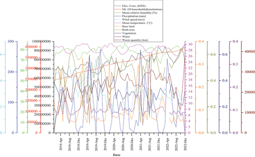
The time series data of disposed MSW has been obtained from the authority of waste management at the engineering landfill center dedicated to host solid waste generated from the study area (i.e., waste quantity in metric ton). In addition, the climatic time series data was obtained from ANAMET (i.e., National Meteorological Agency) based on their availability such as mean temperature (°C), mean relative humidity (%), wind speed (m/s), and precipitation (mm). Also, regarding the socio-economic time series data, the electricity consumption (i.e., Elec. Cons. in kWh) and the number of households and institutions (i.e., Nb. of households&institutions) were collected from CEET (i.e., National Agency for Electric Power). These data were collected on monthly basis from January 2018 to December 2022 and illustrated in Figure 1.

Figure 1. Multivariate time series dataset.

Remote Sensing Features

This study considered the geospatial time series dataset of LULC features such as built area, bare land, vegetation, and water probability indices, as shown in Figure 1. The monthly aggregated time series of probability indices of features’ presence described the dynamic of their importance within the study area. These time series data were computed from the Dynamic World, a near real-time global 10 m LULC mapping project producing land cover probability indices from Sentinel-2 1C, through Google Earth Engine and Artificial Intelligence Platform computation, from January 2018 to December 2022 (Brown et al. 2022).

Pre-Processing

Features Scaling

Before any process with the dataset gathered from the study area, it requires regarding the diversity among those features with different scales, a normalization prior to model’s implementation. The min-max scaling (i.e., normalization) is a way to rescale values ranging from 0 to 1. It subtracts the min value and divides by the max minus the min, while the standardization subtracts the mean value and then divides by the variance. Unlike min-max scaling, the standardization does not bind values to a specific range, which may be a problem for some algorithms (e.g., neural networks often expect an input value ranging from 0 to 1) (Géron and Nicole 2017). In addition, the missing data points observed in the LULC time series patterns were replaced by the mean of each feature and then normalized according to their different nature and order of magnitude.

Pearson Correlation Coefficient Analysis

In multivariate time series problems, several features called independent variables are used to forecast the target variable (i.e., dependent feature). To better understand the relationship among such features, the Pearson correlation coefficient (r) was adopted to measure the linear relationship between features. Its value ranges between (−1) and (+1), where values close to (+1) stand for high positive linear correlation, values close to zero signify a non-linear correlation, and values close to (−1) stand for high negative linear correlation between features (Cai et al. 2020). The Pearson correlation coefficient was computed through Equation (1) as follows:

(1) $\mathit{r}={\sum }_{i=1}^n\left(x_i-\bar{x}\right)(y_i-\bar{y})/\sqrt{{\sum }_{i=1}^n{\left(x_i-\bar{x}\right)}^2}\sqrt{{\sum }_{i=1}^n{\left(y_i-\bar{y}\right)}^2}$(1)

where n represents the total number of records of features $x_i$ and $y_i$ with i = 1, 2…n, their index values, and $\bar{x}$, $\bar{y}$ the average values of $x_i$ and $y_i$, respectively.

Features Selection

There are several techniques of features selection in multivariate time series tasks, which are divided into two categories named “feature screening” and “dimension reduction.” The former is used for the selection of highly correlated features; meanwhile, the latter is used to eliminate the collinearity among features in the pre-processing step (Wang et al. 2023). Hence, in this study, RFR and GBR were considered for feature selection prior to MSW generation forecasting (Dunkel et al. 2022). As a result, the Python programming language with Scikit-Learn library was used because of its stability, flexibility, and provided ensemble learning models ready to use. The selected algorithms for feature selection were subsequently described and implemented under Python environment (see Supplementary materials).

Random Forest Regressor

The use of RFR in feature selection analysis was proven to be the most suitable for different types of data such as solar and wind power data (Wang et al. 2023). This algorithm was implemented in two steps through the computation of node and feature importance, respectively (Dunkel et al. 2022). Based on the decision tree principle, each node’s importance was computed through the Gini score which stands for the average change in node splitting impurity of each feature ($\mathit{ni}$) as illustrated in the case of the binary tree set in Equation (2) as follows:

(2) $\mathit{n}{i}_j=w_j{C}_j-w_{lef{t}_j}{C}_{lef{t}_j}-w_{r\mathrm{igh}{t}_j}{C}_{r\mathrm{igh}{t}_j}$(2)

with $\mathit{n}{i}_j$ the importance of node j, $w_{lef{t}_j}$ and $w_{r\mathrm{igh}{t}_j}$ the weighted number of datasets at the left child and right child of node j, respectively, and $C_{lef{t}_j}$ and $C_{r\mathrm{igh}{t}_j}$ the left child and right child of the Gini impurity values of node j, respectively.

Thereafter, the importance of the features’ coefficient and its normalization (i.e., ranged between 0 and 1) were calculated through Equations (3)(3) $f_{i_i}={\sum }_{\mathit{j}:\mathit{node}\mathit{jsp}\mathit{lits}\mathit{on}\mathit{feature}\mathit{i}}\mathit{n}{i}_j/{\sum }_{\mathit{k}\mathit{\epsilon }\mathit{all}\mathit{nodes}}\mathit{n}{i}_k$(3) and (4(4) $\mathit{norm}\left(f_{i_i}\right)=f_{i_i}/{\sum }_{\mathit{j}\mathit{\epsilon }\mathit{all}\mathit{features}}{f}_{i_j}$(4) ), respectively, as follows:

(3) $f_{i_i}={\sum }_{\mathit{j}:\mathit{node}\mathit{jsp}\mathit{lits}\mathit{on}\mathit{feature}\mathit{i}}\mathit{n}{i}_j/{\sum }_{\mathit{k}\mathit{\epsilon }\mathit{all}\mathit{nodes}}\mathit{n}{i}_k$(3)

(4) $\mathit{norm}\left(f_{i_i}\right)=f_{i_i}/{\sum }_{\mathit{j}\mathit{\epsilon }\mathit{all}\mathit{features}}{f}_{i_j}$(4)

where $f_{i_i}$, $\mathit{n}{i}_j$ are, respectively, the importance of feature $\mathit{i}$ and node $\mathit{j}$.

The overall feature importance resulting from RFR is consequently the average of the calculated feature importance of all decision trees through Equation (5) as follows:

(5) $\mathit{RFR}\left(f_{i_i}\right)={\sum }_{\mathit{j\epsilon }\mathit{all}\mathit{trees}}\mathit{norm}\left(f_{{\mathit{i}}_{\mathit{ij}}}\right)/\mathit{T}$(5)

where $\mathit{RFR}\left(f_{i_i}\right)$ is the final importance of feature $\mathit{i}$ calculated from all trees, $\mathit{norm}\left(f_{{\mathit{i}}_{\mathit{ij}}}\right)$ the normalized feature importance in tree $\mathit{j}$, and $\mathit{T}$ the total number of trees.

The algorithm was implemented through the module “RandomForestRegressor” imported from the Scikit-Learn ensemble under Python environment. The feature importance also called the Gini importance was obtained after fitting the model on the dataset of independent features and target feature, through the function “feature_importances_” giving the score (i.e., normalized values ranged between 0 and 1) of each feature during the regression process considering the default optimized parameters.

Gradient Boosting Regressor

The GBR is based on the gradient boosting algorithm, which consists of minimizing the loss function with a series of weak learners (i.e., decision tree, random forest, etc.) using gradient descent for optimization and better accuracy in regression as well as classification problems (Friedman 2001, 2002). This ensemble learning algorithm can learn non-linear functions in RA by reducing bias and maintaining the low variance through the function shown in Equation (6) as follows:

(6) $f_m\left(\mathit{x}\right)=f_{\mathit{m}-1}\left(\mathit{x}\right)+{\rho }_m\mathit{h}\left(\mathit{x};{\alpha }_m\right)$(6)

where $f_m\left(\mathit{x}\right)$, $\mathit{h}\left(\mathit{x};{\alpha }_m\right)$ are, respectively, the loss function of inputs $\mathit{x}$ and weak-learner, with m = 1, 2, … . n, the iteration number for optimizing the coefficients ${\rho }_m$ and ${\alpha }_m.$

Therefore, the module “GradientBoostingRegressor” was imported from the Scikit-Learn ensemble in Python environment and applied on a set of independent features and target feature. The outputs given by the function “feature_importances_,” were the scores (i.e., ranged between 0 and 1) ascribed to each feature presenting their importance on the targeted feature with respect to the optimized parameters set by default during the RA.

Models’ Implementation

Three neural network models such as LSTM, CNN, and hybrid CNN+LSTM were implemented as baselines alongside the LSTNet-based model for MSW generation forecasting. The models were described through the implemented algorithms as follows (see supplementary materials).

LSTM

Established by Hochreiter and Schmidhuber, the LSTM model is widely used in time series tasks as a particular RNN model for solving long-term dependencies by adding memory cell’s ability with the use of gate mechanism to better monitor the sequence of information. The unroll hidden layer presents an architecture of four interacting layers, instead of one layer that uses the RNN. The four interacting layers were represented by the input (i.e., $i^{\left(\mathit{t}\right)}$), forget (i.e., $f^{\left(\mathit{t}\right)}$), output (i.e., $o^{\left(\mathit{t}\right)}$) gates, and the cell state vector (i.e., $c^{\left(\mathit{t}\right)}$); these gates, respectively, decide whether or not to add new input, what information to erase or add, and output the relevant information at current step $\mathit{t}$ (Hochreiter and Schmidhuber 1997). As a result, the hidden layer output (i.e., $h^{\left(\mathit{t}\right)}$) was obtained through the mathematical formulas shown in Equation (7)(7) $o^{\left(\mathit{t}\right)}=f_g\left(w_o{x}^{\left(\mathit{t}\right)}+u_o{h}^{\left(\mathit{t}-1\right)}+b_o\right)$(7) as follows:

$f^{\left(\mathit{t}\right)}=f_g\left(w_f{x}^{\left(\mathit{t}\right)}+u_f{h}^{\left(\mathit{t}-1\right)}+b_f\right)$

$i^{\left(\mathit{t}\right)}=f_g\left(w_i{x}^{\left(\mathit{t}\right)}+u_i{h}^{\left(\mathit{t}-1\right)}+b_i\right)$

(7) $o^{\left(\mathit{t}\right)}=f_g\left(w_o{x}^{\left(\mathit{t}\right)}+u_o{h}^{\left(\mathit{t}-1\right)}+b_o\right)$(7)

$c^{\left(\mathit{t}\right)}=f^{\left(\mathit{t}\right)}\circ c^{\left(\mathit{t}-1\right)}+i^{\left(\mathit{t}\right)}\circ f_c\left(w_c{x}^{\left(\mathit{t}\right)}+u_c{h}^{\left(\mathit{t}-1\right)}+b_c\right)$

$h^{\left(\mathit{t}\right)}=o^{\left(\mathit{t}\right)}\circ f_h\left(c^{\left(\mathit{t}\right)}\right)$

where $c^{\left(\mathit{t}-1\right)}$, $h^{\left(\mathit{t}-1\right)}$ are, respectively, the cell state and output of the hidden layer at time $\mathit{t}-1$, the coefficients $w_f$, $w_i$, $w_o$, and $w_c$ represent the weights of gates and cell state, and $b_f$, $b_i$, $b_o$, $b_c$ represent their bias. The coefficients $u_f$, $u_i$, $u_o$, $u_c$ are the weights of the interacting layers to connect the hidden layers and outputs successively. $f_g$, $f_c$ represent the sigmoid activation function, and $f_h$ represents the tanh activation function.

CNN

The CNN is commonly used in computer vision tasks, with its two-dimensional CNN architecture, while an alternative one-dimensional CNN is used in natural language processing (e.g., voice recognition, audio generation, etc.) and TSA, which provides feature extraction ability by moving kernel along the time axis (Chung et al. 2014). A simple mathematical formula that represents the one-dimensional convolution along the input signal is a combination of multiplication and addition as shown in Equation (8)(8) $y_j={\sum }_{k=-p}^p{x}_{\mathit{j}-\mathit{k}}{w}_k$(8) :

(8) $y_j={\sum }_{k=-p}^p{x}_{\mathit{j}-\mathit{k}}{w}_k$(8)

where $x_{\mathit{j}-\mathit{k}}$, $y_j$, and $w_k$ are the input, output, and kernel, respectively, with $\mathit{j}$ the index of each sequence, $\mathit{k}$ the index of each element, and $\mathit{p}$ the half of the total elements.

For implementation, a sweeping filter of size 32 and kernel of size 3 with the activation layer of tanh was defined. Then, the 1D maxpooling of size 2 was applied followed by one dense layer with a filter of size 16 and an activation layer of tanh.

CNN+LSTM

The CNN+LSTM architecture used in this study consists of 1D-CNN and LSTM layers where the input sequences were conveyed to the 1D-CNN layer with a filter size of 32, kernel size of 3, and the activation function defined as tanh. Then, 1D-maxpooling with a size of 2 was applied to the output sequences from the 1D-CNN layer followed by a flatten layer to reduce the output dimension. The LSTM layer with a filter size of 32 and activation function tanh was applied with one dense layer after been flattened.

LSTNet

The use of LSTNet model in this study consisted of four main components, which are, respectively, the convolutional, recurrent, recurrent-skip, and autoregressive (AR) components. It is designed for multivariate time series tasks and combines linear and non-linear techniques with the ability to capture long- and short-term patterns (Lai et al. 2018). Its architecture is subsequently described as follows.

The convolutional component consists of sweeping kth filters across the input matrix $\mathit{X}$ using the ReLU activation function (Chung et al. 2014; Lai et al. 2018), as shown in Equation (9)(9) $h_k=\mathit{RELU}\left(W_k\ast \mathit{X}+b_k\right)$(9) :

(9) $h_k=\mathit{RELU}\left(W_k\ast \mathit{X}+b_k\right)$(9)

where $\mathit{RELU}\left(\mathit{x}\right)=\max \left(0,\mathit{x}\right)$, $h_k$ is the output vector by zero padding at the beginning of the input matrix $\mathit{X}$, $W_k$ is the weight matrix connected to the kth feature of the kernel, and $b_k$ is the bias of the feature. The output matrix from this layer is made of each $h_k$.

The output of the convolutional component was fed into the recurrent component defined as the GRU hidden layer, which is composed of the reset gate ($r_t$), update gate ($u_t$), candidate hidden state ($c_t$), and outputs $h_t$ at the current time step $\mathit{t}$ of the hidden layer. Its computation is represented by Equation (10)(10) $u_t=\mathit{\sigma }\left(x_t{W}_{\mathit{xu}}+h_{\mathit{t}-1}{W}_{\mathit{hu}}+b_u\right)$(10) :

$r_t=\mathit{\sigma }\left(x_t{W}_{\mathit{xr}}+h_{\mathit{t}-1}{W}_{\mathit{hr}}+b_r\right)$

(10) $u_t=\mathit{\sigma }\left(x_t{W}_{\mathit{xu}}+h_{\mathit{t}-1}{W}_{\mathit{hu}}+b_u\right)$(10)

$c_t=\mathit{RELU}\left(x_t{W}_{\mathit{xc}}+r_t\odot \left(h_{\mathit{t}-1}{W}_{\mathit{hc}}\right)+b_c\right)$

$h_t=\left(1-u_t\right)\odot h_{\mathit{t}-1}+u_t\odot c_t$

where $\mathit{\sigma }$ is the sigmoid activation function, $x_t$ is the input of the layer at time t; $W_{\mathit{xr}}$, $W_{\mathit{hr}}$, $W_{\mathit{xu}}$, $W_{\mathit{hu}}$, $W_{\mathit{xc}}$, $W_{\mathit{hc}}$ are the matrix weights of the gates and the candidate hidden state connecting the input $x_t$ and the previous hidden state $h_{\mathit{t}-1}$. $b_r$, $b_u$, $b_c$ are the bias terms, and $\odot$ is the element-wise operator. $\mathit{x}$, $\mathit{h}$, $\mathit{r}$, $\mathit{u}$, and $\mathit{c}$ are the input, output, reset gate, update gate, and hidden layer matrices, respectively.

Simultaneously, the recurrent-skip layer like the recurrent layer was fed by the output of the convolution layer, which improves the short-term and long-term patterns extraction in the GRU layer (Lai et al. 2018). This component introduces a temporal skip connection to better capture information flow and hence optimize the recurrent processing. The current hidden state and the adjacent hidden state were connected through the skip-link and computed through Equation (11)(11) $u_t=\mathit{\sigma }\left(x_t{W}_{\mathit{xu}}+h_{\mathit{t}-\mathit{p}}{W}_{\mathit{hu}}+b_u\right)$(11) as follows:

$r_t=\mathit{\sigma }\left(x_t{W}_{\mathit{xr}}+h_{\mathit{t}-\mathit{p}}{W}_{\mathit{hr}}+b_r\right)$

(11) $u_t=\mathit{\sigma }\left(x_t{W}_{\mathit{xu}}+h_{\mathit{t}-\mathit{p}}{W}_{\mathit{hu}}+b_u\right)$(11)

$c_t=\mathit{RELU}\left(x_t{W}_{\mathit{xc}}+r_t\odot \left(h_{\mathit{t}-\mathit{p}}{W}_{\mathit{hc}}\right)+b_c\right)$

$h_t=\left(1-u_t\right)\odot h_{\mathit{t}-\mathit{p}}+u_t\odot c_t$

where $\mathit{p}$ is the number of hidden cells skipped by sweeping the output matrix of the convolutional layer.

The fourth component is the AR model incorporated to combine the non-linear patterns from convolutional and recurrent components, with the linear part describing the local scaling patterns. The AR hidden layer output $h_{t,i}^L$ ${\mathbb{R}}^n$ was computed through Equation (12)(12) $h_{t,i}^L={\sum }_{\mathit{k}=0}^{{\mathit{q}}^{\mathit{ar}}-1}{W}_k^{ar}{Y}_{\mathit{t}-\mathit{k},\mathit{i}}+b^{\mathit{ar}}$(12) :

(12) $h_{t,i}^L={\sum }_{\mathit{k}=0}^{{\mathit{q}}^{\mathit{ar}}-1}{W}_k^{ar}{Y}_{\mathit{t}-\mathit{k},\mathit{i}}+b^{\mathit{ar}}$(12)

where $W^{\mathit{ar}}$, $b^{\mathit{ar}}$ $\mathbb{R}$ are the coefficient of the AR layer, $q^{\mathit{ar}}$ is the window size of the input matrix.

The final forecasting ${\hat{Y}}_{\mathit{t}}$ at the time step $\mathit{t}$ of the LSTNet model was given by combining the outputs of the neural networks and AR components in Eequation (13)(13) ${\hat{Y}}_{\mathit{t}}=h_t^D+h_t^L$(13) as follows:

(13) ${\hat{Y}}_{\mathit{t}}=h_t^D+h_t^L$(13)

where $h_t^D$ is the concatenated result obtained from the recurrent and recurrent-skip by a fully connected layer, and $h_t^L$ is the output of the AR component (Lai et al. 2018).

Post-Processing

Features influence

The IG is used to evaluate feature influence on MSW generation forecasting for results interpretation under neural network models’ implementation. It is a component adding explanatory power to deep neural network models which are known as “Black Box” algorithms. The IG of forecasted values was computed by a function $\mathit{F}$ for a given input $\mathit{x}$ and the baseline $\mathit{x}{ }^{\mathrm{\prime }}$ with respect to the $\mathit{i}$th dimension (Goh et al. 2020), through Equation (14)(14) $\mathit{I}{G}_i\left(\mathit{x},\mathit{x}{ }^{\mathrm{\prime }}\right)::=\left(x_i-x_i^{\prime }\right)\ast {\int }_{\alpha =0}^1\mathrm{\partial }\mathit{F}\left(\mathit{x}{ }^{\mathrm{\prime }}+\mathit{\alpha }\ast \left(\mathit{x}-\mathit{x}{ }^{\mathrm{\prime }}\right)\right)/\mathrm{\partial }{x}_i\mathit{d\alpha }$(14) :

(14) $\mathit{I}{G}_i\left(\mathit{x},\mathit{x}{ }^{\mathrm{\prime }}\right)::=\left(x_i-x_i^{\prime }\right)\ast {\int }_{\alpha =0}^1\mathrm{\partial }\mathit{F}\left(\mathit{x}{ }^{\mathrm{\prime }}+\mathit{\alpha }\ast \left(\mathit{x}-\mathit{x}{ }^{\mathrm{\prime }}\right)\right)/\mathrm{\partial }{x}_i\mathit{d\alpha }$(14)

The easy way to compute the integral is to approximate it by a summation through discretized intervals n with N steps over the straight-line path from the input $\mathit{x}$ to baseline $\mathit{x}{ }^{\mathrm{\prime }}$ through Equation (15):

(15) $\mathit{I}{G}_i\left(\mathit{x},\mathit{x}{ }^{\mathrm{\prime }}\right)\approx \left(x_i-x_i^{\prime }\right)\ast \frac{1}{N}{\sum }_{n=1}^N\mathrm{\partial }\mathit{F}\left(\mathit{x}{ }^{\mathrm{\prime }}+\frac{n}{N}\ast \left(\mathit{x}-\mathit{x}{ }^{\mathrm{\prime }}\right)\right)/\mathrm{\partial }{x}_i$(15)

The baseline input $\mathit{x}{ }^{\mathrm{\prime }}$ chosen here is zero-tensor, which represents a near-zero score for the absence of input features as recommended by researchers (Goh et al. 2020). The algorithm was deployed by importing the module “IntegratedGradients” from “Captum” package under the Python environment. The final IG scores given to each feature resulted from the aggregated scores computed from the batches of inputs on the test set. The absolutes values were explored to assess the intensity of feature influences on the models’ forecasting results.

Evaluation Metrics

To evaluate and benchmark the forecasting accuracy of models, the appropriate metrics selected are, respectively, the root relative squared error (RSE) and root relative absolute error (RAE) (Lai et al. 2018). Equations (16)(16) $\mathit{RSE}=\sqrt{{\sum }_{i=1}^N{\left(Y_i-{\hat{Y}}_{\mathit{i}}\right)}^2}/\sqrt{{\sum }_{i=1}^N{\left(Y_i-\bar{Y}\right)}^2}$(16) , (17(17) $\mathit{RAE}={\sum }_{i=1}^N\left|Y_i-{\hat{Y}}_{\mathit{i}}\right|/{\sum }_{i=1}^N\left|Y_i-\bar{Y}\right|$(17) ) used for computing the corresponding metrics are as follows:

(16) $\mathit{RSE}=\sqrt{{\sum }_{i=1}^N{\left(Y_i-{\hat{Y}}_{\mathit{i}}\right)}^2}/\sqrt{{\sum }_{i=1}^N{\left(Y_i-\bar{Y}\right)}^2}$(16)

(17) $\mathit{RAE}={\sum }_{i=1}^N\left|Y_i-{\hat{Y}}_{\mathit{i}}\right|/{\sum }_{i=1}^N\left|Y_i-\bar{Y}\right|$(17)

where ${\hat{Y}}_{\mathit{i}}$, $\overline{\stackrel{ˆ}{Y}}$ are, respectively, the $\mathit{i}$th forecasted values and their means; $Y_i$, $\bar{Y}$ are, respectively, the $\mathit{i}$th input values and their means, and N is the total length of the input set.

The normalized data were used for the metrics computation on the test set. The lower the values of $\mathit{RSE}$ and $\mathit{RAE}$ are, the better the model performs.

Results and Discussion

Features Correlation and Selection

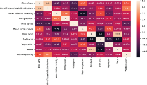
The socio-economic, climatic, and LULC patterns composed of the electricity consumption (i.e., Elec. Cons.), number of households and institutions (i.e., Nb. of households&institutions), mean relative humidity, precipitation, wind speed, mean temperature, bare land, built area, vegetation, and water were used including disposal waste generated (i.e., waste quantity) to find and understand the correlation among them through the Pearson correlation coefficient (r). Figure 2 presented the results of r and the values close to +1 and −1 illustrated the highest linear relationship with a positive slope and negative slope, respectively, while values close to zero showed the non-linear relationship between features. This indicated that the electricity consumption and the number of households and institutions, mean temperature and mean relative humidity, built area and bare land, water and bare land, water and built area are highly correlated with r superior or equal to 0.7 and inferior or equal to −0.7. The ideal linear relationship illustrated with the value 1 was found among the same features. The remaining values of r illustrated the random nature of real-world data, especially when observing r values between waste quantity and all independent features. Only the number of households and institutions showed a relative linear relationship with waste quantity (i.e., r = 0.5). Generally, these results showed a low linear relationship of socio-economic, climatic, and LULC features with MSW generation. Similarly, Cubillos (2020) found that there is no significant linear relationship between weather features (i.e., humidity, temperature, precipitation, and wind speed) and household disposal in Herning, Denmark.

Figure 2. Pearson correlation coefficient of features.

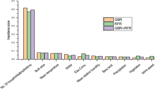
On the other hand, to avoid redundant information from features in MSW generation forecasting, the recommended methods of GBR and RFR were used for feature selection (Wang et al. 2023). Therefore, regardless of the relative importance values obtained, a threshold value of 0.05 was defined to extract the most important features from GBR and RFR analysis. Figure 3 depicts the relative importance scores of the 10 independent features, and the top four selected features under GBR analysis were the number of households and institutions (0.6177), built area (0.0793), mean temperature (0.0709), and water (0.0599). From the RFR analysis, the top four features selected were the number of households and institutions (0.5733), built area (0.0757), mean temperature (0.0734), and electricity consumption (0.0674). Consequently, five features were selected on the average basis from GBR and RFR analysis, which were the number of households and institutions (0.5955), built area (0.0775), mean temperature (0.0722), water (0.0505), and electricity consumption (0.0502). Therefore, the less important features were the mean relative humidity, bare land, precipitation, vegetation, and wind speed. These results indicated the high level of importance of the number of households and institutions from socio-economic features, followed by the built area and mean temperature from LULC and climatic features, respectively. This was highlighted by Lu et al. (2022) who showed that the precipitation, temperature, built area, and household consumption level were important features with scores above the threshold value of 0.05, by implementing the GBRT (Gradient Boosting Regression Tree) for MSW generation rate prediction at multi-city level (Lu et al. 2022).

Figure 3. Features selection from GBR and RFR.

Models’ Performance

The multivariate time series data on monthly basis, composed of 11 features from socio-economic, climatic, and LULC over 5 years, were divided into 80% for the training set and 20% for the test set that corresponds, respectively, to 48 months (i.e., 4 years) and 12 months (i.e., 1 year) of data records. The early stopping method was applied for the baseline models under Keras library, and multiple training runs were applied to LSTNet-based models under the Pytorch library. The dedicated 80% of the training dataset was splitted into 60% for training and 20% for validation regarding the complexity of LSTNet model structure. The overall algorithms were implemented under Python 3.10.12 environment with the hyperparameters presented in Table 1. The performance evaluation was conducted on the LSTNet-based models with its added components such as GBR and RFR for feature selection, and IG for feature influence explanation on forecasted results (i.e., LSTNet+IG, RFR+LSTNet+IG, GBR+LSTNet+IG, and RFR+GBR+LSTNet+IG) alongside the baseline models (i.e., LSTM, CNN, CNN+LSTM). Table 1 shows that LSTNet+IG achieved the best performance with the lowest RSE (0.9727) and RAE (0.9108) values, followed by the RFR+LSTNet+IG (0.9782, 0.9900), RFR+GBR+LSTNet+IG (1.0145, 1.0892), and GBR+LSTNet+IG (1.1873, 1.1903) models, respectively, with their corresponding RSE and RAE values. However, the baseline models achieved better performances compared to the GBR+LSTNet+IG model. Figure 4 illustrates the trend of forecasting results on the test set over 12 months of the year 2022, indicating the ability of the LSTNet+IG model to better mimic the ground truth data patterns.

Figure 4. Models forecasting results on the test dataset.

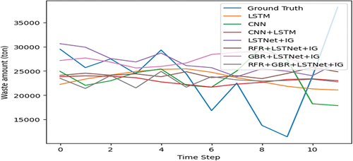
Table 1. Models parameters and performances.

Model	Hyperparameters				Forecasting
	Layer	Optimizer	Activation function	Dropout	RSE	RAE
LSTM	2-layer LSTM (64, 32)	SGD	tanh	0.2	1.0253	1.0708
CNN	1D-CNN (32)	SGD	tanh	0.2	1.1080	1.1727
CNN+LSTM	1D-CNN (32), 1-layer LSTM (32)	SGD	tanh	0.2	1.0134	1.0595
LSTNet+IG	1D-CNN, GRU, GRUskip, Linear	Adam	Sigmoid	0.3	0.9727	0.9108
RFR+LSTNet+IG	1D-CNN, GRU, GRUskip, Linear	Adam	Sigmoid	0.3	0.9782	0.9900
GBR+LSTNet+IG	1D-CNN, GRU, GRUskip, Linear	Adam	Sigmoid	0.3	1.1873	1.1903
RFR+GBR+LSTNet+IG	1D-CNN, GRU, GRUskip, Linear	Adam	Sigmoid	0.3	1.0145	1.0892

Features’ Influence

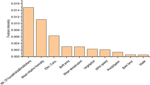
The IG component of the LSTNet+IG model aimed to provide feature influence understanding in the forecasting results interpretation. As mentioned above, the influence scores were averaged over all the model iterations on the test set to give the relative feature influence on MSW generation forecasting. Hence, the absolute values were considered to only explore feature influence intensity on the LSTNet model’s outputs. From the depicted results in Figure 5, the number of households and institutions (0.0149) achieved the highest influence, followed by mean relative humidity (0.0112), electricity consumption (0.0063), built area (0.0030), mean temperature (0.0030), vegetation (0.0023), wind speed (0.0021), precipitation (0.0013), bare land (0.0006), and water (0.0005). The overall low values of feature influence intensity and the high amplitude of the number of households and institutions confirm the moderate and low linear correlation with waste generation, as illustrated by the Pearson correlation coefficient. Among the climatic features, the mean relative humidity and mean temperature achieved the highest influence intensity on model results, which could be explained by the high value of Pearson correlation coefficient, indicating their importance for MSW generation. From LULC features, the built area achieved the highest influence intensity followed by vegetation, bare land, and water.

Figure 5. LSTNet+IG features influence intensity.

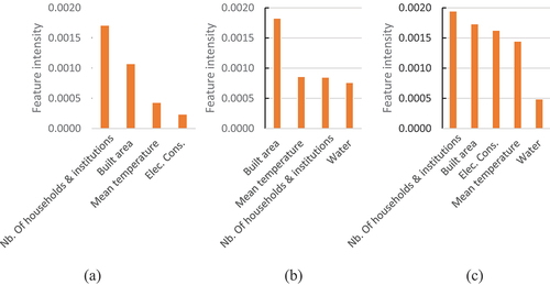
Moreover, Figure 6(a,b,c) presents the influence intensity of selected features on forecasting results from the RFR+LSTNet+IG, GBR+LSTNet+IG, and RFR+GBR+LSTNet+IG models. Among the top four features selected for the RFR+LSTNet+IG model, the number of households and institutions had the highest influence, followed by built area, mean temperature, and electricity consumption (Figure 6(a)). In the case of GBR+LSTNet+IG, the built area was the most influencing feature, followed by the mean temperature, number of households and institutions, and water (Figure 6(b)). Regardless of the top five features considered in the RFR+GBR+LSTNet+IG model, the results showed the number of households and institutions as the most influencing feature, followed by built area, electricity consumption, mean temperature, and water (Figure 6(c)).

Figure 6. (a) RFR+LSTNet+IG features influence, (b) GBR+LSTNet+IG features influence, and (c) RFR+GBR+LSTNet+IG features influence.

However, from the results of RFR and GBR feature selection techniques, the mean relative humidity was not recorded as one of the key influencing features probably due to the existing collinearity with the mean temperature as confirmed by the Pearson correlation coefficient (r = −0.7). This could be the reason for the low performance of RFR+LSTNet+IG, GBR+LSTNet+IG, and RFR+GBR+LSTNet+IG models. The best performance of the LSTNet+IG model could be explained by its ability to capture all features patterns and learn from complex data as confirmed by Wang et al. (2023). Moreover, the RFR technique showed better feature screening ability that led to the good performance of the RFR+LSTNet+IG model when compared with GBR+LSTNet+IG and RFR+GBR+LSTNet+IG models, as confirmed by Wang et al. (2023). Overall, the top five key influencing features given by the LSTNet+IG model were the number of households and institutions, mean relative humidity, electricity consumption, built area, and mean temperature. Indeed, the socio-economic features largely influenced the LSTNet+IG model results as confirmed by Hoang et al. (2017), followed by the mean relative humidity, mean temperature from climatic features, and the built area from LULC features (Hoang et al. 2017). As a result, the mean relative humidity regarding the overall feature influence intensities from the LSTNet+IG model among the climatic features achieved the most influencing amplitude ahead of the mean temperature, precipitation, and wind speed. However, Vu, Ng, and Bolingbroke (2019) in their study on MSW generation forecasting found the temperature as the most relevant feature, followed by the precipitation and humidity from climatic features (Vu, Ng, and Bolingbroke 2019). In addition, Han et al. (2018) in their study demonstrated that the temperature and the related consumption patterns such as electricity consumption had high influence on MSW generation (Han et al. 2018). Moreover, Johnson et al. (2017) in their study on weekly waste generation forecasting in New York City with the Gradient Boosting model, found that the most significant feature used was the temperature and showed that the demographic and socio-economic features were in contrast uninformative for short-term forecasting (Johnson et al. 2017). Despite the satisfactory results explanation conducted with the IG component added to the LSTNet model, this study did not investigate feature influence direction on forecasting results owing to the lack of long-term historical time series data availability. This could be further explored for a better understanding of the relationship between feature patterns variability and MSW generation trends from the study area with large-scale data.

Conclusion

MSW generation forecasting has challenged stakeholders and researchers in developing appropriate tools to better understand the involved patterns from socio-economic, climatic, and LULC features. Indeed, this study implemented LSTNet+IG, RFR+LSTNet+IG, GBR+LSTNet+IG, and RFR+GBR+LSTNet+IG, alongside the baseline models such as LSTM, CNN, and CNN+LSTM, to fill the gap of conventional and black box nature of RNN techniques and MSW disposal data availability. The results showed that LSTNet+IG with the lowest RSE (0.9727) and RAE (0.9108) values outperformed others and demonstrated its ability to better extract feature patterns in MSW generation forecasting. However, the RFR and GBR techniques for feature selection did not improve the LSTNet-based models; instead, they achieved low performance owing to the reduced dataset size. In addition, the RFR technique has proved to be the best compared to GBR and RFR+GBR through their corresponding LSTNet-based models (i.e., GBR+LSTNet+IG and RFR+GBR+LSTNet+IG). On the other hand, from the IG component, we found five key influencing features on the overall forecasting results obtained in the order of decreased amplitude: the number of households and institutions, mean relative humidity, electricity consumption, built area, and mean temperature. Moreover, from the socio-economic, climatic, and LULC features, the number of households and institutions, mean relative humidity, and built area showed the highest amplitude on MSW generation forecasting. This study demonstrated the influences of socio-economic, climatic, and LULC features on MSW generation, which need to be taken into consideration by stakeholders to anticipate and mitigate the issues of waste stream mismanagement and disseminate best practices with appropriate resource allocation to communities. However, further investigation will be conducted to understand the relationship between feature patterns variability and MSW generation trend and improve forecasting results on large-scale data.

Acknowledgements

The authors are grateful to the German Federal Ministry of Education and Research (BMBF) through the West African Science Service Centre on Climate Change and Adapted Land Use (WASCAL) for financial support, and would like to acknowledge the authorities of DAGL, ANAMET, and CEET for providing the data required for this study.

Disclosure Statement

No potential conflict of interest was reported by the author(s).

Supplementary Material

Supplemental data for this article can be accessed online at https://doi.org/10.1080/08839514.2024.2387504.

Data Availability Statement

Data is made available publicly.

References

- Abbasi, M., and M. A. Abduli. 2013. Forecasting municipal solid waste generation by hybrid support vector machine and partial least square model. International Journal of Environmental Research 7 (1):27–21.
- Abbasi, M., M. A. Abduli, B. Omidvar, and A. Baghvand. 2014. Results uncertainty of support vector machine and hybrid of wavelet transform-support vector machine models for solid waste generation forecasting. Environmental Progress & Sustainable Energy 33 (1):220–28. doi:10.1002/EP.11747.
- Abbasi, M., and A. El Hanandeh. 2016. Forecasting municipal solid waste generation using artificial intelligence modelling approaches. Waste Management 56:13–22. doi:10.1016/J.WASMAN.2016.05.018.
- Abdulkareem, K. H., M. A. Subhi, M. A. Mohammed, M. Aljibawi, J. Nedoma, R. Martinek, M. Deveci, W. L. Shang, and W. Pedrycz. 2024. A manifold intelligent decision system for fusion and benchmarking of deep waste-sorting models. Engineering Applications of Artificial Intelligence 132:107926. doi:10.1016/J.ENGAPPAI.2024.107926.
- Adusei, K. K., K. T. W. Ng, N. Karimi, T. S. Mahmud, and E. Doolittle. 2022. Modeling of municipal waste disposal behaviors related to meteorological seasons using recurrent neural network LSTM models. Ecological Informatics 72:101925. doi:10.1016/J.ECOINF.2022.101925.
- Ali Abdoli, M., M. Falah Nezhad, R. Salehi Sede, and S. Behboudian. 2012. Longterm forecasting of solid waste generation by the artificial neural networks. Environmental Progress & Sustainable Energy 31 (4):628–36. doi:10.1002/EP.10591.
- Al-Mashhadani, I. B. 2023. Waste material classification using performance evaluation of deep learning models. Journal of Intelligent Systems 32 (1). doi:10.1515/jisys-2023-0064.
- Brown, C. F., S. P. Brumby, B. Guzder-Williams, T. Birch, S. B. Hyde, J. Mazzariello, W. Czerwinski, V. J. Pasquarella, R. Haertel, S. Ilyushchenko, et al. 2022. Dynamic world, near real-time global 10 m land use land cover mapping. Scientific Data 2022 9:1, 9 (1):1–17. doi:10.1038/s41597-022-01307-4.
- Cai, J., K. Xu, Y. Zhu, F. Hu, and L. Li. 2020. Prediction and analysis of net ecosystem carbon exchange based on gradient boosting regression and random forest. Applied Energy 262:114566. doi:10.1016/j.apenergy.2020.114566.
- Choi, H., C. Jung, T. Kang, H. J. Kim, and I. Y. Kwak. 2022. Explainable time-series prediction using a residual network and gradient-based methods. Institute of Electrical and Electronics Engineers Access 10:108469–82. doi:10.1109/ACCESS.2022.3213926.
- Chung, J., C. Gulcehre, K. Cho, and Y. Bengio. 2014. Empirical evaluation of gated recurrent neural networks on sequence modeling. ArXiv preprint arXiv:1412.3555v1:1–9. doi:10.48550/arXiv.1412.3555.
- Cubillos, M. 2020. Multi-site household waste generation forecasting using a deep learning approach. Waste Management 115:8–14. doi:10.1016/J.WASMAN.2020.06.046.
- Dunkel, J., D. Dominguez, Ó. G. Borzdynski, and Á. Sánchez. 2022. Solid waste analysis using open-access socio-economic data. Sustainability (Switzerland) 14 (3). doi:10.3390/su14031233.
- Friedman, J. H. 2001. Greedy function approximation: A gradient boosting machine. Annals of Statistics 29 (5):1189–232. doi:10.1214/aos/1013203451.
- Friedman, J. H. 2002. Stochastic gradient boosting. Computational Statistics & Data Analysis 38 (4):367–78. doi:10.1016/S0167-9473(01)00065-2.
- Géron, A. 2017. Hands-on machine learning with scikit-learn and TensorFlow, ed. T. Nicole, 1st ed. Sebastopol, CA, USA: O’Reilly Media, Inc.
- Goh, G. S. W., S. Lapuschkin, L. Weber, W. Samek, & A. Binder. 2020. Understanding integrated gradients with smoothtaylor for deep neural network attribution. Proceedings - International Conference on Pattern Recognition, 4949–56. doi:10.1109/ICPR48806.2021.9413242.
- Han, Z., Y. Liu, M. Zhong, G. Shi, Q. Li, D. Zeng, Y. Zhang, Y. Fei, and Y. Xie. 2018. Influencing factors of domestic waste characteristics in rural areas of developing countries. Waste Management 72:45–54. doi:10.1016/J.WASMAN.2017.11.039.
- Hoang, M. G., T. Fujiwara, S. T. Pham Phu, and K. T. Nguyen Thi. 2017. Predicting waste generation using Bayesian model averaging. Global Journal of Environmental Science and Management 3 (4):385–402. doi:10.22034/gjesm.2017.03.04.005.
- Hochreiter, S., and J. Schmidhuber. 1997. Long short-term memory. Neural Computation 9 (8):1735–80. doi:10.1162/NECO.1997.9.8.1735.
- Hockett, D., D. J. Lober, and K. Pilgrim. 1995. Determinants of per capita municipal solid waste generation in the Southeastern United States. The Journal of Environmental Management 45 (3):205–17. doi:10.1006/jema.1995.0069.
- Izquierdo-Horna, L., R. Kahhat, and I. Vázquez-Rowe. 2022. Reviewing the influence of sociocultural, environmental and economic variables to forecast municipal solid waste (MSW) generation. In Sustainable production and consumption, vol. 33, 809–19. Elsevier B.V. doi:10.1016/j.spc.2022.08.008.
- Johnson, N. E., O. Ianiuk, D. Cazap, L. Liu, D. Starobin, G. Dobler, and M. Ghandehari. 2017. Patterns of waste generation: A gradient boosting model for short-term waste prediction in New York City. Waste Management 62:3–11. doi:10.1016/J.WASMAN.2017.01.037.
- Kumar, N. M., M. A. Mohammed, K. H. Abdulkareem, R. Damasevicius, S. A. Mostafa, M. S. Maashi, and S. S. Chopra. 2021. Artificial intelligence-based solution for sorting COVID related medical waste streams and supporting data-driven decisions for smart circular economy practice. Process Safety and Environmental Protection 152:482–94. doi:10.1016/J.PSEP.2021.06.026.
- Lai, G., W. C. Chang, Y. Yang, and H. Liu. 2018. Modeling long- and short-term temporal patterns with deep neural networks. 41st International ACM SIGIR Conference on Research and Development in Information Retrieval, SIGIR 2018, 95–104. doi:10.1145/3209978.3210006.
- Lin, K., Y. Zhao, L. Tian, C. Zhao, M. Zhang, and T. Zhou. 2021. Estimation of municipal solid waste amount based on one-dimension convolutional neural network and long short-term memory with attention mechanism model: A case study of Shanghai. Science of the Total Environment 791:148088. doi:10.1016/J.SCITOTENV.2021.148088.
- Lu, W., W. Huo, H. Gulina, and C. Pan. 2022. Development of machine learning multi-city model for municipal solid waste generation prediction. Frontiers of Environmental Science & Engineering 16 (9):1–10. doi:10.1007/s11783-022-1551-6.
- Mohammed, M. A., M. J. Abdulhasan, N. M. Kumar, K. H. Abdulkareem, S. A. Mostafa, M. S. Maashi, L. S. Khalid, H. S. Abdulaali, and S. S. Chopra. 2023. Automated waste-sorting and recycling classification using artificial neural network and features fusion: A digital-enabled circular economy vision for smart cities. Multimedia Tools & Applications 82 (25):39617–32. doi:10.1007/s11042-021-11537-0.
- Niu, D., F. Wu, S. Dai, S. He, and B. Wu. 2021. Detection of long-term effect in forecasting municipal solid waste using a long short-term memory neural network. Journal of Cleaner Production 290:125187. doi:10.1016/j.jclepro.2020.125187.
- Rahman, A. U., M. Saeed, M. A. Mohammed, K. H. Abdulkareem, J. Nedoma, and R. Martinek. 2023. Fppsv-NHSS: Fuzzy parameterized possibility single valued neutrosophic hypersoft set to site selection for solid waste management. Applied Soft Computing 140:110273. doi:10.1016/J.ASOC.2023.110273.
- Shahabi, H., S. Khezri, B. Ahmad, and H. Zabihi. 2012. Application of artificial neural network in prediction of municipal solid waste generation (case study: Saqqez city in Kurdistan Province). World Applied Sciences Journal 20 (2):336–43.
- Sun, Q., and Z. Ge. 2021. Deep learning for industrial KPI prediction: When ensemble learning meets semi-supervised data. IEEE Transactions on Industrial Informatics 17 (1):260–69. doi:10.1109/TII.2020.2969709.
- Tseng, F. M., H. C. Yu, and G. H. Tzeng. 2002. Combining neural network model with seasonal time series ARIMA model. Technological Forecasting & Social Change 69 (1):71–87. doi:10.1016/S0040-1625(00)00113-X.
- Vu, H. L., K. T. W. Ng, and D. Bolingbroke. 2019. Time-lagged effects of weekly climatic and socio-economic factors on ANN municipal yard waste prediction models. Waste Management 84:129–40. doi:10.1016/J.WASMAN.2018.11.038.
- Wang, D., Y. A. Yuan, Y. Ben, H. Luo, and H. Guo. 2022. Long short-term memory neural network and improved particle swarm optimization–based modeling and scenario analysis for municipal solid waste generation in Shanghai, China. Environmental Science and Pollution Research 29 (46):69472–90. doi:10.1007/s11356-022-20438-0.
- Wang, H., W. Fu, C. Li, B. Li, C. Cheng, Z. Gong, Y. Hu, and H. Dinçer. 2023. Short-term wind and solar power prediction based on feature selection and improved long- and short-term time-series networks. Mathematical Problems in Engineering 1–7. doi:10.1155/2023/7745650.
- Xu, A., H. Chang, Y. Xu, R. Li, X. Li, and Y. Zhao. 2021. Applying artificial neural networks (ANNs) to solve solid waste-related issues: A critical review. In Waste management, vol. 124, 385–402. Elsevier Ltd. doi:10.1016/j.wasman.2021.02.029.