Modelling Deceleration in Senescent Mortality

Abstract

Mortality deceleration is the observed but yet to be understood phenomenon that the increase in the late-life death rate slows down after a certain species-related advanced age. Various definitions of onsets of mortality deceleration are examined. A new distribution based on the Strehler-Mildvan theory of aging takes on the required shapes. The application is done on mortality data from the 1892 cohort of Swedish women and on Mediterranean fruit flies.

Keywords:

• biodemography
• Gompertz law
• mortality deceleration
• mortality rate
• onset of late-life mortality
• senescent mortality

1. INTRODUCTION

Gompertz (1825) proposed a simple model of mortality with age:

where μ(x)dx is the probability that an individual who has reached the age x dies between age x and age x + dx. This is the force of mortality, also known in survival analysis as the hazard rate function. Its survival function is defined as , where X is the lifetime, and the probability density function is .

Eq. (1) was augmented by Makeham (1867) with the addition of a constant to model age-independent mortality. This appears to fit reasonably well with human and other organisms between sexual maturity and some advanced age. Late-life mortality may not follow a Gompertz law (Greenwood and Irwin, 1939). Mortality would decelerate along various trajectories rather than merely plateau (Vaupel et al., 2004), and it is better to consider departure from the Gompertz law rather than just convergence of mortality to a plateau level.

As direct calculation of mortality rates at advanced ages is problematic due to sampling error inherent in small surviving cohort sizes (Wilmoth, 1995), models are substituted for the highest ages in mortality tables. Non-Gompertzian late-life mortality models (Yashin et al., 2000) are of four types:

1. “Change-point models,” where mortality changes from Gompertzian to something else at a given point. Economos (1982) modelled late-life mortality as exponentially decreasing. Steinsaltz (2005) suggested a constant rate after a threshold, or a change to a Gompertz of different age-dependent parameter.

2. Models with a “decay” or “tapering” term added to the Gompertz law. For example, the “logistic frailty model” (Vaupel et al., 1979):

   the “logistic model” (Thatcher, 1999):
   the “logistic Gompertz” (Steinsaltz, 2005):
   and the logistic regression model of Himes et al. (1994):
   where Y _j (x) is the logit transformation of death rates at age x to x + 1 in population j, and δ, (β _x ) _x , and (γ _j ) _j are coefficients to be estimated.

3. Models with mixtures:

   1. the type of Heligman and Pollard (1980) and Witten (1988), where different life phases are represented by different mixture components (Witten and Eakin, 1997). In the Heligman and Pollard (1980) model, late-life mortality is linearly increasing with age (Thatcher, 1999), while in the Witten (1988) model it is constant. Bebbington et al. (2007a) distinguished exogenous from endogenous causes (Carnes et al., 2006). The endogenous component follows a “Flexible Weibull” distribution (Bebbington et al., 2007b), which is asymptotically equivalent to the Gompertz law. Later life mortality was from both component distributions, with some exogenous effects assumed to become more lethal with advancing age.

   2. the frailty models (Vaupel et al., 1979), where the “frailty” parameter A in Eq. (1) varies from individual to individual according to a gamma distribution; α being identical for all individuals. This results in Eq. (2), with A in Eq. (2) different from that in Eq. (1). The versions fitted to data were discrete mixtures (Kowald and Kirkwood, 1993; Vaupel and Carey, 1993). The idea is that in heterogeneous models less robust individuals tend to die off earlier (Steinsaltz and Wachter, 2006).

4. The models of reliability and survival analysis (Lai and Xie, 2006). Among these, the Weibull model:

   implies a monotonic mortality. Nonmonotonic models include bathtub shapes (Bebbington et al., 2007c) with decreasing infant mortality and increasing late-life mortality, and upside down bathtub distributions with decreasing late-life mortality. The latter includes the lognormal distribution, whose force is
   (Lai and Xie, 2006), the Birnbaum-Saunders (Bebbington et al., 2008a), inverse Gaussian, log-logistic, Burr XII, the truncated normal (Fox and Moya-Larano, 2003), and phase type distributions (Aalen, 1995).

Choice of model rather than the data has dictated the shape of the mortality acceleration or deceleration. We will define mortality deceleration and test a new distribution that can take on many possible shapes.

2. ACRONYMS

Right-tail shapes:

• UIA: Ultimately increasing and accelerating;

• UID: Ultimately increasing and decelerating;

• UD: Ultimately decreasing (or, equivalently, ultimately declining)

Onsets:

• ODA: Onset of decreasing acceleration;

• ODV: Onset of decreasing velocity;

• ONV: Onset of negative velocity

3. ONSETS OF MORTALITY DECELERATION

3.1. Definitions Based on the Force of Mortality

Witten (1989) defined “acceleration of aging” as , by treating the force of mortality μ as “velocity.” Hence an analogous measure of “acceleration of mortality” is the second derivative .

Definition 1

The force of mortality μ is ultimately increasing and accelerating (UIA) if and only if there is an age x* such that μ′(x) > 0 and μ″(x) > 0 for all x > x*. Under these circumstances, we say that there is no onset of late-life deceleration.

Definition 2

The force of mortality μ is ultimately increasing but decelerating (UID) if and only if there is an age x** such that μ′(x) > 0 and μ″(x) < 0 for all x > x**. The smallest x** is denoted by x _ODV and called the onset of decreasing velocity. The first local maximum of the function μ″ to the left of x _ODV is called the onset of decreasing acceleration, denoted by x _ODA.

Definition 3

The force of mortality μ is ultimately decreasing (UD) if and only if there exists an age x*** such that μ′(x) < 0 for all x > x***. The smallest such x*** is denoted by x _ONV and called the onset of negative velocity or the onset of decline. The first point to the left of x _ONV where the function μ″ becomes zero is called the onset of decreasing velocity, denoted by x _ODV. The first local maximum of the function μ″ to the left of x _ODV is called the onset of decreasing acceleration, denoted by x _ODA.

These definitions do not apply to change point models at the change point, only beyond this point. An extension is to define the change point as a point of deceleration if:

where x _c is the change point. The model of Steinsaltz (2005):

with α₁ > α₂, has a deceleration point at x _c , but is UIA. As mortality models are intended to apply to large groups of individuals, where it is biologically implausible that all individuals will have the same change point, we focus on smooth mortality functions.

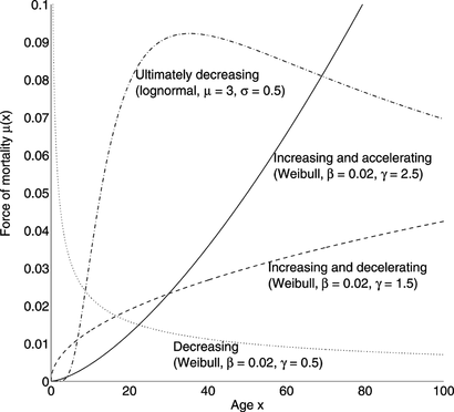
All upside down bathtub distributions are ultimately decreasing, where x _ONV is the point at which μ attains its maximum. The Weibull distribution in Eq. (6) has derivatives and . Thus the Weibull is UIA if 2 < γ, UID (with x _ODV = 0) if 1 < γ ≤ 2, and UD (with x _ONV = 0) if γ ≤ 1. Examples are shown in Figure 1.

FIGURE 1 Examples of accelerating and decelerating forces of mortality.

The exponential distribution μ(x) = constant is neither accelerating, decelerating, or decreasing; the Gompertz distribution in Eq. (1) is increasing and accelerating .

The three models in Eq. (2-4) are amenable to analysis:

	The logistic frailty model is defined by Eq. (2), which has the first derivative: and thus μ is decreasing when α < As 2, constant when α = As 2, and increasing when α > As 2. The second derivative is: The case α = As 2 is trivial. When α < As 2, μ″ is positive. When α > As 2, there is a unique solution to at as for all x > x 0. When α < As 2, μ in Eq. (2) is UD with the onset of negative velocity x ONV = 0. When α > As 2, μ is UID, with the onset of decelerating velocity: Eq. (2) is not capable of UIA behavior.
	The force of mortality of the logistic model in Eq. (3) is always increasing because is always positive. The second derivative is: When A ≥ 1, then for all x > 0, but when A < 1, there is a unique solution to at: as for all x > x 0. The force of mortality in Eq. (3) is always UID, with the onset of decelerating velocity
	The logistic Gompertz model in Eq. (4) has the first derivative which implies that μ is decreasing when A < B, constant when A = B, and increasing when A > B. The second derivative is: The case A = B is trivial. When A < B, then μ in Eq. (4) is decreasing with the onset of negative velocity x ONV = 0. When B ≥ 1, then for all x > 0. When B < 1, there is a unique solution to at: noting that for all x > x 0. Consider the case A > B. When B ≥ 1, for all x > 0, but when B < 1, there is a unique solution to at x 0, with for all x > x 0. Hence, when A < B, then μ in Eq. (4) is UD with the onset of negative velocity x ONV = 0. When A > B, μ in Eq. (4) is UID, with the onset of decreasing velocity Again, Eq. (4) cannot be ultimately increasing and accelerating.

As the three models yield monotonic forces of mortality they cannot be used to estimate a mortality rate which first increases then decreases. As models in Eq. (2-4) are all either decreasing or ultimately decelerating, they cannot be used to determine whether mortality is decelerating.

3.2. Other Definitions of Mortality Acceleration

Horiuchi and Coale (1990) use the age-specific rate of mortality change with age (or life-table aging rate):

with the onset of deceleration being defined as the point at which μ′/μ begins to decrease. However, a change-point model may not always be appropriate. Witten (1989) compares the force of mortality of a cohort under consideration with respect to a “baseline” mortality function. This is the definition for mortality deceleration in humans with the Gompertz law.

Another measure of mortality deceleration is provided by the life expectancy:

If the life expectancy increases, the mortality is certainly decelerating (Carey et al., 1992). For upside down bathtub shaped μ, provided μ(0) < 1/e ₀, then e _x is of bathtub shape (Gupta and Akman, 1995), and the minimum of e _x occurs before the maximum of μ (Mi, 1995). A monotonically increasing force of mortality has a monotonically decreasing life expectancy, so that we cannot distinguish between acceleration and deceleration in the sense of Definitions 1 and 2 using e _x . Furthermore, an increasing life expectancy e _x is not a sufficient condition for μ to be decreasing; e _x must also be concave .

A measure of the rate of senescence is the time required for the mortality to double (Finch et al., 1990). Table 1 gives the mortality rate of decrement for some distributions, with increasing forces of mortality.

TABLE 1 Mortality Rate of Decrement (MRD)

Distribution	Force of mortality μ	MRD
Gompertz	αe ^βx	(1/β)ln 2
Weibull (γ > 1)	γβ(βx)^γ−1	(2^1/(γ−1))x
Linear	λ1 + λ2 x	λ1/λ2 + x

Eakin and Witten (1995a) used the curvature of the survival function to create a time-scaling on which they defined a gerontological distance. The extremal points of the curvature of this scaled survival function are used to define a region where the slope of the survival function is maximal, and approximately constant (Eakin and Witten, 1995b).

This procedure is known as ‘rectangularity’, and is interpreted in terms of the genetically predetermined species life-span. Bebbington et al. (2006) used the extremal points of the curvature of the survival, force of mortality, and life expectancy functions to define useful life periods in reliability engineering. Bebbington et al. (2007a) identified life phases, among which is the onset of late-life deceleration. The curvature function for the force of mortality μ is:

and we define the onset of decreasing velocity as the right-most zero of the curvature function κ_μ, which coincides with the definition based on μ″. However, the onset of decreasing acceleration as the right-most local extremum of κ_μ(x) may differ from the point identified with μ″.

4. BIODEMOGRAPHIC EXPLANATIONS OF AGING

We have already mentioned that change point models may imply the existence of a point at which some biological quantity varies with age in a nondifferentiable, if not discontinuous, manner. While this is reasonable in individuals due to gene expression changes during aging, it is unlikely to occur in all members of a population at the same age.

4.1. Heterogeneity Versus Natural Selection—Mixture Models

Carey et al. (1992), and Curtsinger et al. (1992) conducted large scale experiments on the mortality of flies. The populations involved were large enough to provide late-life mortality data on sufficiently large number of individuals. Vaupel et al. (1998) put forward mortality correlation, heterogeneity in frailty, and induced demographic schedules.

Rauser et al. (2006) and Olshansky and Carnes (1997) reviewed various theories of late life evolution, dividing them into those based on natural selection and those based on lifelong heterogeneity. Both are mixture distributions. The former mixes age-specific survival probabilities over subsequent age classes, while the latter mixes a parameter in the force of mortality over the population by assigning a prior distribution to the parameter.

Mueller and Rose (1996) derived various age-specific rates as a consequence of selection, mutation, and genetic drift with mortality plateaus, after initial Gompertzian aging. However, age-independent beneficial effects appear necessary for a plateau in the force of mortality to occur at a level less than one per time interval, which is extinction (Charlesworth, 2001). Fox and Moya-Larano (2003) presented deceleration as a consequence of the normal distribution of lifetimes produced by considering the lifetime as the sum of random effects of a large number of genes. However, human lifetimes are not normally distributed (figure 1 in Horiuchi, 2003).

4.2. Strehler-Mildvan Theory

Strehler and Mildvan (1960) suggested a relationship between “vitality” v(x) and mortality of the form:

A linear decline in vitality:

into Eq. (25) produces the Gompertz law of Eq. (1).

Weitz and Fraser (2001) generalized the linear decay to a Wiener process with drift, resulting in a model with mortality plateau or a upside down bathtub shape. The addition of a repair rate, likewise decreasing linearly with age, produces an exponential-quadratic mortality function (Horiuchi, 2003). Golubev (2009) suggests a “generalized Gompertz law,” where the mortality has an age-dependent factor Λ(x), resulting in the force of mortality:

5. A FLEXIBLE LATE-LIFE MORTALITY LAW

We search for a distribution whose force of mortality can represent a variety of shapes, which could be ultimately increasing, leveling off, or decreasing. Late-life mortality is difficult to estimate, as only a small portion of the data is representative.

Rather than positing a linear decline in vitality as in Eq. (26) coupled with a repair or replacement function, we combine both in the form:

where c, d > 0 are parameters (Vaupel et al., 2004). The function of Eq. (28) is nonnegative, and allows a variation in the rate of the net decline in vitality with age. We assume an age-related mortality factor:

in the generalized Gompertz law of Eq. (27), with , resulting in the force of mortality:

where the Makeham parameter a ≥ 0 avoids biasing the estimate of mortality acceleration with the effect of intrinsic mortality (Pletcher, 1999; Hallen, 2009), and modifies the life expectancy (Bebbington et al., 2008b). It is unnecessary to include A ₀, because the resulting force of mortality is simply rescaled on the x-axis and reparameterized in terms of c. It is convenient to take A ₀ = d c ^−(b+1)/d .

The force of mortality of Eq. (30) corresponds to the survival function:

where is the upper incomplete gamma function. Substituting results in:

where the subscript Γ refers to the gamma function. Differentiating, the force of mortality is:

When b* < 0 (b > −1), the upper incomplete Gamma function Γ(b*, y) → ∞ when y → 0, while if b* > 0 (b < −1), the integral exists even when y = 0. This enables the distribution to take on a variety of shapes. While b*, or more generally 1 + db* = −b is a shape parameter, c is a location parameter, which controls the age-scaling of the force of mortality. We have always μ_Γ(0) = a.

To study the possible shapes of μ_Γ, we calculate its first derivative:

where . Hence, the sign of is the same as ψ₁(x ^d ). The second derivative:

where . The sign of is the same as ψ₂(x ^d ), which is a quadratic polynomial in x ^d .

Even if we restrict the parameters to

the force of mortality μ_Γ achieves all the desired late-life aging shapes.

The shape of μ is independent of a which can be set to 0 as in Eq. (36). We also have . In particular, μ_Γ is increasing on the entire positive half-line if and only if , and is upside down bathtub shaped if and only if , with its maximum attained at the point x _ONV = 1/(1 + b*).

Theorem 1

If Eq. (36) holds, then

1. When b* ≤ −2, then the force of mortality μ_Γ is ultimately increasing and accelerating; that is, its first and second derivatives are positive on the entire positive real half-line.

   1. If b* < −2, then μ_Γ grows to infinity and is asymptotically convex downwards (has positive second derivative) in x, or

   2. if b* = −2, then μ_Γ grows to infinity, but is asymptotically linear (second derivative tends to zero) in x.

2. When b* ∈ (−2, −1], then μ_Γ is ultimately increasing but decelerating.

   1. If b* ∈ (−2, −1), then μ_Γ grows to infinity and is asymptotically concave downwards (has negative second derivative), or

   2. if b* = −1, then μ_Γ increasingly approaches when x → ∞.

   3. The acceleration is positive on the interval [0, x _ODV) and negative on (x _ODV, ∞), where .

3. When b* > −1, then μ_Γ is ultimately decreasing.

   1. μ_Γ starts decreasing at x _ONV = 1/(1 + b*).

   2. The acceleration is zero at , and also at .

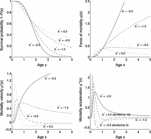
The survival functions, force of mortality and their derivatives are shown in Figure 2 for the cases in Theorem 1.

FIGURE 2 Shapes of distribution Eq. (32), with a = 0, c = d = 1.

6. EXAMPLES

We have chosen one example with ultimately increasing but decelerating behavior, and one with ultimately decreasing behavior.

6.1. Swedish Mortality Data

Death rates for the 1892 cohort of Swedish women were obtained from the Human Mortality Database. These were fit directly to the various forces of mortality by minimizing the sum of squares. Steinsaltz (2005) discusses truncation at some initial age before fitting, but the truncation point then becomes a parameter which potentially affects mortality. Instead we used the sum-of-squares method to reduce the influence on the parameters from the large number of shorter life spans.

The fitted and empirical μ are shown in Figure 3. While the Weibull and lognormal distributions fit the data poorly, the force of mortality μ_Γ and Eq. (2-4) perform similarly, and the differences are at younger ages. The estimated parameters are given in Table 2.

FIGURE 3 Fit to Swedish death rates of various forces of mortality. Eq. (2-4) are almost overlying.

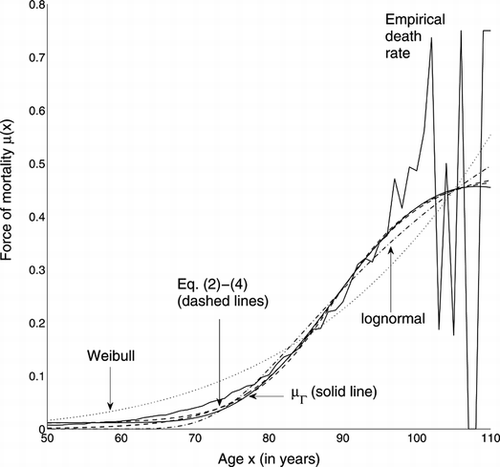
TABLE 2 Estimated Parameters for Swedish Mortality Data

Distribution	Parameters
μΓ	a = 0.018, b = 5.01, c = 2.5 × 10^5, d = 2.29
Weibull	γ = 0.014, β = 5.48
Lognormal	μ = 4.39, σ = 0.077
Logistic frailty	s = 0.569, A = 4.3 × 10^−7, α = 0.157
Logistic	γ = 0.011, k = 0.465, A = 1.9 × 10^−7, α = 0.174
Logistic Gompertz	k = 6.2 × 10^−4, A = 7.2 × 10^−4, B = 9.2 × 10^−7, α = 0.156

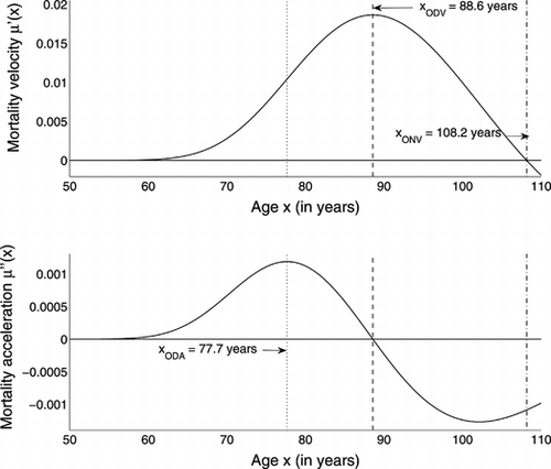
The velocity corresponding to μ_Γ and its acceleration are shown in Figure 4. The acceleration of mortality begins to decrease at about 78 years. The force of mortality begins to decelerate at 89 years and begins to decrease at 108 years, but the data extend to only 110 years.

FIGURE 4 Velocity of μ_Γ (top panel) and its acceleration (bottom panel).

6.2. Medfly Data

On Swedish mortality data, the distribution μ_Γ provides a similar mortality deceleration as existing models of Eq. (2-4). The advantage of the distribution μ_Γ lies in its flexibility to provide various shapes. In order to test this we need mortality data with a greater range of very long lifetimes. Carey et al. (1992: 459) provide mortality data on more than 1.2 million medflies. The insights for demography from such data are summarized by Carey (1997).

The force of mortality of Eq. (33) was fitted to the raw data by maximum likelihood (Pletcher, 1999). The fitted and the empirical μ are shown in Figure 5. The force of mortality μ_Γ is a better fit than the lognormal force of mortality, although it still understates the deceleration. As in the previous example, the Weibull is constrained by the start at μ(0) = 0, and the concavity of the initial section of the mortality curve, to take on an accelerating shape which is a miss-match to the data. Although the Weibull can take on accelerating, decelerating, or decreasing shape, it fails to fit the empirical hazard in this example, as do the models of Eq. (2-4). The estimated parameters are given in Table 3.

FIGURE 5 Fit to Medfly Data of Various Forces of Mortality. Eq. (2-4) are overlying.

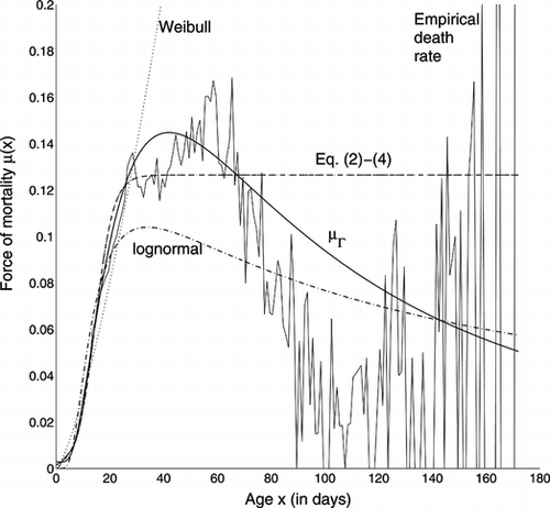
TABLE 3 Estimated Parameters for Medfly Mortality Data

Distribution	Parameters
μΓ	a = 0.003, b = 5.01, c = 36.0, d = 0.425
Weibull	γ = 0.043, β = 2.36
Lognormal	μ = 2.93, σ = 0.484
Logistic frailty	s = 1.536, A = 0.002, α = 0.299
Logistic	γ = 5.4 × 10^−15, k = 0.127, A = 0.013, α = 0.299
Logistic Gompertz	k = 1.9 × 10^−67, A = 8.6 × 10^63, B = 0.013, α = 0.299

Vaupel and Carey (1993) and Kowald and Kirkwood (1993) fitted a mixture of Gompertzian frailty groups to explain the observed mortality deceleration using a cohort heterogeneity explanation. These have 23 and 15 parameters, respectively.

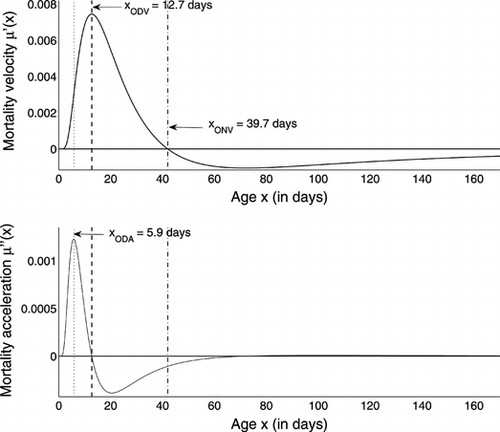
The velocity corresponding to μ_Γ and its acceleration are shown in Figure 6. The latter begins to decrease at about 5.9 days, at which point less than 2.5% of the population has died. The force of mortality begins to decelerate at about 12.7 days (approximately 18% mortality in the population), and the force of mortality begins to decrease at about 39.7 days, at which stage less than 4% of the population survives.

FIGURE 6 Velocity of μ_Γ (top panel) and its acceleration (bottom panel).

7. CONCLUSION

We have outlined three definitions which capture the idea of mortality deceleration. The three zeros x _ODA < x _ODV < x _ONV corresponding to the jerk , acceleration , and velocity μ′, identify the onsets of decreasing acceleration, decreasing velocity, and negative velocity which separate the various life phases. Alternative calculations of the latter two are made using the force of mortality.

The definitions identify the lack of a general distribution displaying accelerating, decelerating, and decreasing shapes; the Weibull distribution fits poorly for mortality data. Excepting infant mortality, the mortality distribution μ_Γ of Eq. (33) captures many possible shapes of late-life mortality. It can be used to detect mortality deceleration, as shown by fitting for mortality data, of the 1892 cohort of Swedish women, and of the medfly data.

ACKNOWLEDGMENTS

Ričardas Zitikis' research was supported by the Natural Sciences and Engineering Research Council (NSERC) of Canada.

REFERENCES

- Aalen , O.O. ( 1995 ). Phase type distributions in survival analysis . Scandinavian Journal of Statistics , 22 : 447 – 463 .
- Bebbington , M. , Lai , C.D. , and Zitikis , R. ( 2006 ). Useful periods for lifetime distributions with bathtub shaped hazard rate functions . IEEE Transactions on Reliability , 55 : 245 – 251 .
- Bebbington , M. , Lai , C.D. , and Zitikis , R. ( 2007a ). Modeling human mortality using mixtures of bathtub shaped failure distributions . Journal of Theoretical Biology , 245 : 528 – 538 .
- Bebbington , M. , Lai , C.D. , and Zitikis , R. ( 2007b ). A flexible Weibull extension . Reliability Engineering and System Safety , 92 : 719 – 726 .
- Bebbington , M. , Lai , C.D. , and Zitikis , R. (2007c). Bathtub curves in reliability and beyond. Australian and New Zealand Journal of Statistics , 49: 251–265.
- Bebbington , M. , Lai , C.D. , and Zitikis , R. ( 2008a ). A proof of the shape of the Birnbaum-Saunders hazard rate function . The Mathematical Scientist , 33 : 49 – 56 .
- Bebbington , M. , Lai , C.D. , and Zitikis , R. ( 2008b ). Reduction in mean residual life in the presence of a constant competing risk . Applied Stochastic Models in Business and Industry , 24 : 51 – 63 .
- Carey , J.R. ( 1997 ). What demographers can learn from fruit fly actuarial models and biology . Demography , 34 : 17 – 30 .
- Carey , J.R. , Liedo , P. , et al. . ( 1992 ). Slowing of mortality rates at older ages in large medfly cohorts . Science , 258 : 457 – 461 .
- Carnes , B.A. , Holden , L.R. , et al. . ( 2006 ). Mortality partitions and their relevance to research on senescence . Biogerontology , 7 : 183 – 198 .
- Charlesworth , B. ( 2001 ). Patterns of age-specific means and genetic variances of mortality rates predicted by the mutation-accumulation theory of aging . Journal of Theoretical Biology , 210 : 47 – 65 .
- Curtsinger , J.W. , Fukui , H.H. , et al. . ( 1992 ). Demography of genotypes: Failure of the limited life-span paradigm in Drosophila melanogaster . Science , 258 : 461 – 463 .
- Eakin , T. and Witten , M. ( 1995a ). A gerontological distance metric for analysis of survival dynamics . Mechanisms of Ageing and Development , 78 : 85 – 101 .
- Eakin , T. and Witten , M. ( 1995b ). How square is the survival curve of a given species? Experimental Gerontology , 30 : 33 – 64 .
- Economos , A.C. ( 1982 ). Rate of aging, rate of dying and the mechanism of mortality . Archives of Gerontology and Geriatrics , 1 : 3 – 27 .
- Finch , C.E. , Pike , M.C. , and Witten , M. ( 1990 ). Slow mortality rate accelerations during aging in animals approximate that of humans . Science , 249 : 902 – 905 .
- Fox , C.W. and Moya-Larano , J. ( 2003 ). Why organisms show late-life mortality plateaus: A null model for comparing patterns of mortality . Evolutionary Ecology Research , 5 : 999 – 1009 .
- Greenwood , M. and Irwin , J.O. ( 1939 ). The biostatistics of senility . Human Biology , 11 : 1 – 23 .
- Golubev , A. ( 2009 ). How could the Gompertz-Makeham law evolve . Journal of Theoretical Biology , 258 : 1 – 17 .
- Gompertz , B. ( 1825 ). On the nature of the function expressive of the law of human mortality, and on a new mode of determining the value of life contingencies . Philosophical Transactions of the Royal Society of London , 115 : 513 – 585 .
- Gupta , R.C. and Akman , H.O. ( 1995 ). Mean residual life functions for certain types of non-monotonic ageing . Communications in Statistics – Stochastic Models , 11 : 219 – 225 .
- Hallen , A. ( 2009 ). Makeham's addition to the Gompertz law re-evaluated . Biogerontology , 10 : 517 – 522 .
- Heligman , L. and Pollard , J.H. ( 1980 ). The age pattern of mortality . Journal of the Institute of Actuaries , 107 : 49 – 80 .
- Himes , C.L. , Preston , S.H. , and Condran , G.A. ( 1994 ). A relational model of mortality at older ages in low mortality countries . Population Studies , 48 : 269 – 291 .
- Horiuchi , S. ( 2003 ). Interspecies differences in the life span distribution: Humans versus invertebrates . Population and Development Review, (Supplement – Life Span: Evolutionary, Ecological and Demographic Perspectives) , 29 : 127 – 151 .
- Horiuchi , S. and Coale , A.J. ( 1990 ). Age patterns of mortality for older women: An analysis using age-specific rate of mortality change with age . Mathematical Population Studies , 2 : 245 – 267 .
- Human Mortality Database. University of California, Berkeley (USA), and Max Planck Institute for Demographic Research (Germany). Retrieved from www.mortality.org
- Kowald , A. and Kirkwood , T.B.L. ( 1993 ). Explaining fruit fly longevity . Science , 260 : 1664 – 1665 .
- Lai , C.D. and Xie , M. ( 2006 ). Stochastic Ageing and Dependence for Reliability . New York : Springer .
- Makeham , W.L. ( 1867 ). On the law of mortality . Journal of the Institute of Actuaries , 13 : 325 – 367 .
- Mi , J. ( 1995 ). Bathtub failure rate and upside-down residual life . IEEE Transactions on Reliability , 44 : 388 – 391 .
- Mueller , L.D. and Rose , M.R. ( 1996 ). Evolutionary theory predicts late-life mortality plateaus . Proceedings of the National Academy of Sciences of the USA , 93 : 15249 – 15253 .
- Olshansky , S.J. and Carnes , B.A. ( 1997 ). Ever since Gompertz . Demography , 34 : 1 – 15 .
- Pletcher , S.D. ( 1999 ). Model fitting and hypothesis testing for age-specific mortality data . Journal of Evolutionary Biology , 12 : 430 – 439 .
- Rauser , C.L. , Mueller , L.D. , and Rose , M.R. ( 2006 ). The evolution of late-life . Ageing Research Reviews , 5 : 14 – 32 .
- Steinsaltz , D. ( 2005 ). Re-evaluating a test of the heterogeneity explanation for mortality plateaus . Experimental Gerontology , 40 : 101 – 113 .
- Steinsaltz , D. and Wachter , K.W. ( 2006 ). Understanding mortality rate deceleration and heterogeneity . Mathematical Population Studies , 13 : 19 – 37 .
- Strehler , B.L. and Mildvan , A.S. ( 1960 ). General theory of mortality and aging . Science , 132 : 14 – 21 .
- Thatcher , A.R. ( 1999 ). The long-term pattern of adult mortality and the highest attained age (with discussion) . Journal of the Royal Statistical Society, Series A , 162 : 5 – 43 .
- Vaupel , J.W. ( 1997 ). Trajectories of mortality at advanced ages . In K.W. Wachter and C.E. Finch (Eds.), Between Zeus and the Salmon: The Biodemography of Longevity . Washington , DC : National Academy Press , pp. 17 – 37 .
- Vaupel , J.W. and Carey , J.R. ( 1993 ). Compositional interpretations of medfly mortality . Science , 260 : 1666 – 1667 .
- Vaupel , J.W. , Manton , K.G. , and Stallard , E. ( 1979 ). The impact of heterogeneity in individual frailty on the dynamics of mortality . Demography , 16 : 439 – 454 .
- Vaupel , J.W. , Carey , J.R. , et al. . ( 1998 ). Biodemographic trajectories of longevity . Science , 280 : 855 – 860 .
- Vaupel , J.W. , Baudisch , A. , et al. . ( 2004 ). The case for negative senescence . Theoretical Population Biology , 65 : 339 – 351 .
- Weitz , J.S. and Fraser , H.B. ( 2001 ). Explaining mortality rate plateaus . Proceedings of the National Academy of Sciences of the USA , 98 : 15383 – 15386 .
- Wilmoth , J.R. ( 1995 ). Are mortality rates falling at extremely high ages? An investigation based on a model proposed by Coale and Kisker . Population Studies , 49 : 281 – 295 .
- Witten , M. ( 1988 ). A return to time, cells, systems, and aging: V. Further thoughts on Gompertzian survival dynamics—the geriatric years . Mechanisms of Ageing and Development , 46 : 175 – 200 .
- Witten , M. ( 1989 ). Quantifying the concepts of rate and acceleration/deceleration of aging . Growth, Development and Aging , 53 : 7 – 16 .
- Witten , T.M. and Eakin , T. ( 1997 ). Multiphasic models of survival: Analysis of mortality rate change regions and the issue of finite species lifespan . Experimental Gerontology , 32 : 259 – 285 .
- Yashin , A.I. , Iachine , I.A. , and Begun , A.S. ( 2000 ). Mortality modeling: A review . Mathematical Population Studies , 8 : 305 – 332 .