Mandibular ecomorphology in the genus ursus (Ursidae, Carnivora): relevance for the palaeoecological adaptations of cave bears (U. spelaeus) from Scladina cave

ABSTRACT

Considerable morphological and ecological diversity has been found in extinct and extant members of the bear genus, Ursus, and appears to be key in explaining how they have thrived across vast ecological gradients. One example is the cave bear Ursus spelaeus. We applied 2D geometric morphometric techniques to describe morphological changes in the mandibles of extant Ursus species to further interpret the palaeoecology of U. spelaeus. Ursus species were discriminated using their mandibular morphology, which showed intra and interspecific shape variation that was indirectly linked to climatic adaptations through dietary variation. Mandibles of bears that inhabit colder, drier and more seasonal environments were generally slender with large diastema and a dorsoventrally smaller ramus. In contrast, species from warmer environments with higher levels of precipitation were found to have a dorsoventrally taller ramus (relative to the corpus). Discriminant function analyses of the morphology of U. spelaeus suggested adaptations to a series of fluctuating environments through time, helping to assess previously proposed Marine Isotope Stages for sedimentary deposits in Scladina Cave. Our geometric morphometrics analyses of bear mandibular ecomorphology demonstrates how geometric morphometrics provides a valuable tool to enhance paleoenvironmental reconstructions within deposits of the same fossil site.

KEYWORDS:

• Quaternary
• palaeoclimate
• evolutionary ecology
• mandible
• geometric morphometrics
• Carnivora

Introduction

Extant and extinct members of the genus Ursus have populated almost every ecological niche across the Holarctic region (Pasitschniak-Arts 1993), from dense forest to open grasslands and polar ice sheets, displaying associated morphological adaptations.

Their large geographic range is due to a relatively recent radiation during the Pliocene. All extant Ursus species share a common ancestor, Ursus minimus Devèze de Chabriol and Bouillet 1827, which underwent cladogenesis leading to several daughter species (Croizet and Jobert 1828; Martin 1989; Baryshnikov and Lavrov 2013), including the living Asian black bear Ursus thibetanus (Cuvier 1823), the American black bear Ursus americanus (Pallas 1780; McLellan and Reiner 1994), the brown bear Ursus arctos (Linnaeus 1758), the polar bear U. maritimus (Phipps 1774) and several extinct bears including the Etruscan bear Ursus etruscus (Cuvier 1823; Baryshnikov 2007) and the cave bears Ursus deningeri and Ursus spelaeus (Rosenmüller 1794; Reichenau 1904; Azzaroli 1983; Martin 1989; Hänni et al. 1994; McLellan and Reiner 1994; Rossi and Santi 2001; Bon et al. 2008). Ursus minimus gave rise to the Etruscan bear in the late Pliocene while cave bear species split from U. arctos around 1-2mya (Loreille et al. 2001; Bon et al. 2008), with U. maritimus later branching from U. arctos (Hailer et al. 2012; Miller et al. 2012; Liu et al. 2014; Kumar et al. 2017; Rinker et al. 2019).

The taxonomy of cave bears has been addressed by several studies due to its geographic variability throughout the Pleistocene. Recent morphological and genetic studies have recognised distinct species, sub-species and multiple evolutionary lineages including: Ursus kudarensis, Ursus deningeri, Ursus rossicus, Ursus ladincus and Ursus spelaeus (Rabeder et al. 2004, 2008, 2010, 2011; Valdiosera et al. 2008; Knapp et al. 2009; Baryshnikov and Puzachenko 2011; Dabney et al. 2013; Stiller et al. 2014). Their diet has also been a topic of great debate for many years, with recent research largely suggesting that species such as U. spelaeus were omnivorous but predominantly consumed plant material (Kurtén 1968; Bocherens et al. 1997, 2006, 2014; Garsia 2003; Raia 2004; Figueirido et al. 2009; Peigné et al. 2009; Rabeder et al. 2010; Meloro 2011; Baryshnikov and Puzachenko 2011; Bocherens 2015, 2019; Charters et al. 2019, 2022; Pérez-Ramos et al. 2019, 2020a, 2020b; van Heteren and Figueirido 2019).

A broad level of morphological variation has been identified within cave bear fossils of the same locality due to the climatic oscillations exhibited over several stratigraphic sequences, supporting subtle dietary shifts in relation to food availability. Shape change was particularly evident in the sequence of Scladina Cave (Belgium) where shape changes in upper and lower molars have been detected in intervals covering less than 100,000 years (Charters et al. 2019, 2022). Fossil mandibles of cave bears are equally abundant in Scladina; however, their morphological variation has not yet been investigated in detail. Meloro et al. (2017) recently identified substantial polymorphism in the mandible shape of Ursidae, which appeared to be associated with climatic adaptations. This framework should allow better interpretation of the morphology of fossil cave bears, whose shape might be indicative of adaptations towards cold or temperate climatic conditions.

Our aim is to interpret morphological variation of fossil cave bears in relation to present day bears ecogeographical patterns. By predicting the ‘optimal’ climatic niche to which cave bear morphology could have been adapted, we aim to interpret its temporal variation in relation to Pleistocene climatic shifts. We predict that if the cave bears underwent adaptive responses to dramatic climatic changes, this should be reflected in climate-correlated changes in mandibular morphology. Extrapolation of this method can also help us understand whether (before their extinction) cave bears were unable to rapidly adapt to the colder conditions and associated changes, including biotic effects (such as increased competition from species such as from humans and brown bear). Our aim is to test for changes in morphology of U. spelaeus and assess whether morphological changes are linked to climatic variation. As all cave bear specimens are from Scladina cave, there is limited geographical influence on diet, which would allow us to interpret morphological change as an indirect link to climate. We expect cave bear fossil mandibles from colder climatic sequences to differ in shape from specimens representative of more temperate conditions, along a gradient of shape changes that can be identified in representative extant species of Ursus. Variation in size is also expected, although due to the larger size variation in cave bears, this variable may not follow comparable patterns in extant species.

Materials and methods

Sites and specimens

A total of 153 hemi-mandibles from one extinct and four extant species of the genus Ursus were used for geometric morphometric analyses including: Ursus americanus, Ursus arctos, Ursus maritimus, Ursus thibetanus and Ursus spelaeus (Figure 1, Table 1, and Table S1). Specimens were examined from nine depositories: Museo Nacional de Ciencias Naturales, Madrid, Spain; Museo Nazionale preistorico Entografico Luigi Pigorini, Roma, Italy; Parco Nazionale d’Abruzzo Lazio & Molise, Abruzzo, Lazio, Italy; Natural History Museum London, UK; American Museum of Natural History, New York, U.S.A.; Scladina Cave Archaeological Centre, Andenne, Namur, Belgium; Museum of Zoology of Torino University, Turin, Italy; World Museum Liverpool, UK and National Museum of Natural History, Sofia, Bulgaria.

Figure 1. Map of the Northern Hemisphere with locations of samples used in this study. Extant species are represented by circles and fossil species represented by triangles.

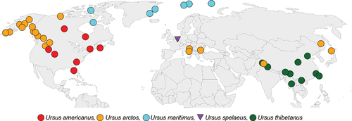
Table 1. Specimens used for this study by species and skeletal element from the mandible, i.e. whole mandible, Corpus only and Ramus only.

Species	Whole	Corpus	Ramus
U. americanus	16	16	15
U. arctos	70	73	70
U. maritimus	16	16	16
U. spelaeus	10	31	12
U. thibetanus	14	15	14
Total	126	151	127

Due to incompleteness of some cave bear specimens, we used three datasets for the analyses: i) whole hemi-mandibles, ii) the corpus only, iii) the ramus only. This allowed us to considerably increase the numbers of U. spelaeus specimens from chronostratigraphic sedimentary units/layers of Scladina Cave, Belgium. Specimens span multiple stratigraphic units from 2A to 7A (Pirson et al. 2008, 2014). For the stratigraphic log including a full synthesis of chronostratigraphical and palaeoenvironmental data see Pirson et al. (2014).

In brief, the majority of deposits found in Scladina Cave have been found to relate to the Upper Pleistocene (Pirson et al. 2014) with Units 7B to 6C been suggested to position in the Middle Pleistocene, possibly Late Saalian (MIS 6; Haesaerts 1992; Pirson 2007; López-García et al. 2017). Unit 6B and possibly part of Unit 6A have been further suggested as a wooded temperate to boreal environment based on analyses of palynology, taxa presence and speleothem growth (Bastin 1992; Cordy 1992; Simonet 1992; Pirson et al. 2008, 2014; López-García et al. 2017). Unit 5 is interpreted as a cooler, steppe period with less tree cover and presence of arctic taxa, while pollen data from Unit 4B indicate arid open steppe conditions (Bastin 1992; Cordy 1992; Pirson 2007; Pirson et al. 2008, 2014). Strong climatic improvement is seen throughout layers within Units 4A-AP and 4A-IP. Palynology (including pollen spectra from stalagmitic floor CC4), large mammals, small mammals and herpetofauna suggest a temperate forest environment with a higher humidity (Bastin 1992; Cordy 1992; Pirson 2007; Pirson et al. 2008, 2014, Blain et al. 2014; López-García et al. 2017). Unit 3-INF in palynology is represented by boreal species, indicating an open boreal environment, while 3-SUP transitions to a more steppic environment with some boreal trees (Pirson 2007; Pirson et al. 2008). To the top of 3-SUP (3-ORH and 3-ORA), a climatic improvement is suggested through palynology, anthracology and the presence of a speleothem (Pirson 2007; Pirson et al. 2008). Unit 2A is considered as a deposit of the Weichselian pleniglacial and Unit 2B suggesting the end of MIS 5a.

Specimens used herein pertain to single or groups of units and not specific stratigraphic layers that correspond to single environmental signatures (in some cases they can encompass several layers with variable climatic signals). This is due to the fossil material being excavated, collected and curated before the reappraisal of the stratigraphy (as in López-García et al. 2017).

Landmark configuration

Each hemi-mandible was photographed using a tripod mounted Nikon D3100 equipped with a 55-200 mm Nikon AF-S DX Zoom (f/4–5.6 G ED) lens and photographs were collected at a fixed 100 mm focal length. The same procedure was carried out for all individuals at all institutions to standardise the collection of image data and minimise error. Intra-observer error was tested on a random subset of specimens (n = 20) and tested by repeated measures in R (ver. 4.1.1) using the packages Geomorph (ver. 4.0) and RRPP (ver. 1.0), showing high levels of repeatability (r² (%) = 99.9) (Table S4).

For analyses, left hemi-mandibles were mirrored so that all specimens had the same orientation. 12, 8 and 6 landmarks (Cartesian coordinates of anatomically homologous points) were digitised on the whole mandible, corpus and ramus specimen datasets, respectively. Landmark coordinates preserve the geometry of the set configuration in the dataset, allowing for effective visual representations of shape and related deformations (Bookstein 1991, 1996; Rohlf and Marcus 1993; Zollikofer and Ponce de Leon 2002; Adams et al. 2004; Zelditch et al. 2004; Slice 2007; Mitteroecker and Gunz 2009). In regard to landmark configuration and justification, a landmark was not placed between P₄ and M₁ due to the fractured nature, wear (karst geological processes) and loss of dentition in most of cave bear specimens.

The software tpsDIG2 (version 2.32; Rohlf 2015) was used to place two-dimensional landmark positions on each specimen, conducted by a single operator (D.C.) to alleviate inter-observer error. Landmarks 1–8 are anatomically placed, while landmarks 9–12 are geometrically aligned projections perpendicular to landmarks 1–4 as the base of the corpus lacks defining morphological features. Whole mandible specimens contain all 12 landmarks and are included in all three datasets, while corpus data use landmarks 1–4, 9–12 and ramus specimens use landmarks 4–9 (Figure 2 and Table 2). Landmark 1 could also be placed on all ‘ramus only’ specimens due to the nature of the preservation of fossil specimens having damage to the mandible around the positions of landmarks 10–12, which excluded them from being used in the whole mandible and corpus datasets, but allowed for the correct placement of landmarks 4 and 9.

Figure 2. (left) anatomical nomenclature of right hemi-mandible and (right) landmark configuration for hemi-mandibles in lateral view (U. spelaeus - SC 92-503-01). Scale bar: 4.0cm. Refer to Table 2 for landmark definitions.

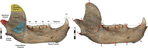
Table 2. Definition and numbering sequence of landmarks for lateral hemi-mandibles.

Landmark	Definition
1	Posterior point of the canine alveolus
2	Anterior point of P4 alveolus
3	Tip of alveolus between M1 and M2
4	Posterior point of M3 alveolus
5	Tip of coronoid process
6	Dorsal extreme of the mandibular condyle
7	Most posterior point of the mandibular condyle
8	Most posterior point of the angular process
9	Perpendicular projection of landmark 4 on the ventral edge of the mandibular corpus based on the line 1–4
10	Perpendicular projection of landmark 3 on the ventral edge of the mandibular corpus based on the line 1–4
11	Perpendicular projection of landmark 2 on the ventral edge of the mandibular corpus based on the line 1–4
12	Perpendicular projection of landmark 1 on the ventral edge of the mandibular corpus based on the line 1–4

Geometric morphometrics (GMM)

All analyses were conducted separately on each mandibular element. Size information was extracted from the raw coordinates using the square root of the sum of squared distances between the landmarks and the centroid (Mitteroecker et al. 2013), with logarithmic transformation (natural logarithm) used to ensure that the distribution in shape space was isotropic. The resultant centroid size (logCS) was used as a measure of size across all datasets. Through Generalized Procrustes analysis (GPA), a Procrustes superimposition was performed, with translation and scaling of all landmarks to the same centroid, then a rotation of all configurations of each specimen to minimise shape distances between them (Gower 1975; Rohlf and Slice 1990). The Generalized Procrustes analysis produced a new set of coordinates named Procrustes coordinates which effectively described spatial positioning of each landmark after removing differences in orientation and size of the specimens. Shape variation between specimens was explored through a principal components analysis (PCA) of Procrustes shape coordinates for each landmark configuration (whole mandible, corpus and ramus) in MorphoJ (ver. 1.06d, Klingenberg 2011, 2013). Principal components analysis reduces the dimensionality of large datasets and produces orthogonal vectors that describe variation within a multivariate sample. Deformation grids based on thin-plate spline were employed to graphically show the mean shape configuration and deformation from the mean at the extremities of each visualised Principal Component (Klingenberg 2013).

Procrustes ANOVA was adopted to test factors (e.g. species) that might impact on variation in mandible shape of the genus Ursus using the R (ver. 4.1.1; R Core Team 2021) packages: Geomorph (ver. 4.0) and RRPP (ver. 1.0) (Adams et al. 2013, 2022; Adams and Collyer 2015; Collyer and Adams 2018, 2019, 2021; Baken et al. 2021; R Core Team 2021) on shape variables, accompanied by pairwise permutations (using residual randomisation with 1000 permutations) further computed in the R package RRPP. These Pairwise comparisons maintain the same type I error rates across model effects and post hoc pairwise comparisons (Collyer et al. 2015) and do not require further p value adjustment to reduce the type I error rate.

A test of allometry (ANOVA using residual randomisation) was also produced in R (ver. 4.1.1; R Core Team 2021) using log transformed centroid size and Procrustes coordinates in order to assess the statistical association between shape and size in species of Ursus. This was followed by pairwise permutation tests in RRPP (ver. 1.0; Collyer and Adams 2018, 2019, 2021).

Ecogeographical variation

For this study, we recorded all geographical data when the information was available in order to assess the ecogeographical variation across species of extant Ursus. This provided us with 119 specimens from the original 153 used in GMM which could be assigned to a total of 49 distinct localities. Sex was not determined for specimens of U. spelaeus due to the preservation of the hemi-mandibles (broken and lack of important sexually dimorphic elements such as canines) at the time of data collection. To circumvent the important factor of sex, we used allometrically corrected shape variables in all analyses. Residuals produced from linear regression on Procrustes coordinates and log centroid size were retained and used in place of standard Procrustes coordinates as this removes the largely sexually dimorphic factor of size in the data set. This was conducted on all U. spelaeus and extant species to ensure sex is not a confounding factor influencing any climatic interpretations. Landmark configurations for extant specimens (within the same location) were further averaged by location (to avoid pseudo-replications) and tests between species groups used group means for shape, size and allometric tests to reduce the impact of sexual dimorphism (see Cáceres et al. 2014; Meloro et al. 2017).

Nineteen bioclimatic variables were extracted for each location and used in subsequent analyses as a proxy for climate (see Table S2 for bioclimatic variable definitions). These bioclimatic variables were extracted at a resolution of 2.5 minutes from the WorldClim database of current climate (~1950–2000; Hijmans et al. 2005) using DIVA-GIS 7.5 (Hijmans et al. 2001, 2012) software. Each of the 19 bioclimatic variables were converted to the standardised normal distribution (i.e. $\mathit{z}=\frac{\mathit{x}-\mathit{\mu }}{\sigma }$) prior to any analyses to avoid weighting differences of any variable. Separate linear regressions were first employed to test associations between each bioclimatic parameter and extant bear shape variables. Only variables with statistically significant association between bioclimatic variables and shape variables were retained and included in Partial Least Squares analysis, while non-significant bioclimatic variables were seen as redundant (see Table S3). For example, bioclimatic variables such as ‘driest month’ may be related to summer or winter, and such may or may not be during torpor. Linear regression is used to clarify if the bioclimatic variable shows statistically significant association with shape variables which would then result in that bioclimatic variable being valid or not in analyses. This allowed selection of only relevant bioclimatic variables in subsequent partial least squares (PLS) analyses (see Meloro and Sansalone 2022).

Partial least squares analysis is a technique that allows the extraction of pairs of vectors which maximise covariation between two blocks of multivariate datasets (Rohlf et al. 2000). Here, PLS is applied to find covariation between climate and mandible shape variables. Initially, a Two-Block PLS analysis was conducted on only statistically significant standardised bioclimatic variables and allometrically corrected Procrustes coordinates of extant bear species in the software MorphoJ (ver 1.06d; Klingenberg 2011, 2013). Partial least square vector scores (PLS1 and 2 of block 1 [shape data] and PLS1 and 2 of block 2 [climate data]) were retained. A linear regression was then run on all allometrically corrected Procrustes coordinates (extant species and U. spelaeus) against PLS1 of block 1. From this analyses, the unstandardised predicted values were retained for all bear specimens. The same was repeated for PLS2 of block 1. The unstandardised predicted PLS values of U. spelaeus were then plotted (projected) relative to extant bear species. The same plotting was done using the unstandardised predicted values of cave bears against PLS1 of block 2. Ursus spelaeus was plotted on a regression line as it has been extrapolated from a previous regression of PLS1 block 1 vs PLS1 block 2 (shape only). This process was then repeated for each dataset (whole mandible, corpus and ramus).

A spread of U. spelaeus was expected along the predicted regression line due to specimens pertaining to multiple different chronostratigraphic sedimentary units of Scladina Cave that were settled during different climatic conditions. Discriminant function analyses (DFA) were additionally performed using allometrically corrected PLS1 and PLS2 morphology scores as independent variables and Köppen-Geiger climate classifications (simplified to five main groups to allow for more robust classifications: Tropical, Arid, Temperate, Cold and Polar) given to extant ursid species as predictor variables for palaeoclimate classification of U. spelaeus. The ‘Tropical’ classification was not applicable to any specimens of our dataset. Köppen-Geiger climate classifications are divided groups and sub-group categories that maps biome distributions around the world based on threshold values of air temperature, precipitation and topographic effects (Köppen 1936; Peel et al. 2007; Beck et al. 2018; Fig. S1). Cross-validated classifications were identified for each extant bear location and simplified classifications were used for DFA. These have been derived from multiple high-resolution climatic datasets (WorldClim V1 and V2, CHELSA V1.2, and CHPclim V1; Hijmans et al. 2005; Funk et al. 2015; Fick and Hijmans 2017; Karger et al. 2017). Using PLS1 and PLS2 morphology vector scores of extant Ursus, DFA was employed to statistically predict climate categories for U. spelaeus specimens based on their shape. Climatic predictions using logCS were not produced due to the size of U. spelaeus specimens being generally larger than extant Ursus species.

Results

Mandibular shape in ursids

Principal components analysis scatter plots evidenced a certain level of species discrimination across both PC1 and PC2 in morphospace for all datasets (whole mandible, corpus and ramus) (Figure 3). For the whole mandible, corpus and ramus, 95% of total shape variance was covered in the first 11, 7 and 7 PC vectors, respectively.

Figure 3. PCA plot of mandibular morphology across species for the (a) whole mandible (b) corpus and (c) ramus. Allometry plots of PC1 against logCS for (d) whole mandible, (e) corpus and (f) ramus. Deformation grids and two-coloured wireframes show mean shape (light blue) and deformation (dark blue) at the extremity of each axis for each PC.

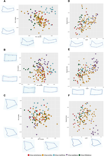
For the whole mandible, positive PC1 (23.12% var) describes an anteroposterior expansion and a dorsoventral contraction of the corpus. Positive scores on PC2 (16.99% var) reflect an expansion of the diastema, with negative scores indicating an anteroposterior expansion of the ramus relative to mean shape. In this dataset, the cave bear (U. spelaeus) groups with U. arctos and U. thibetanus, dominating the morphospace of negative PC1 and positive PC2 as a result of a contracted shape of the corpus at the molars and an expansion of the diastema. The Asian black bear (U. thibetanus) specimens possess negative scores on PC1, reflecting a dorsoventrally thicker corpus. Overlap between U. arctos and U. americanus specimens occurs around the centre of the morphospace. The majority of U. maritimus specimens are differentiated by positive PC1/PC2 scores, indicating an expanded diastema and thinner corpus body relative to mean shape.

For the corpus, the PCA scatter plot (PC1 35.48% var, PC2 30.81% var.) manifested major overlap for most species around the origin of the PC axes. All U. thibetanus show negative PC1 scores while the polar bear (U. maritimus) shows positive scores due to an expanded diastema and anteroposterior lengthening relative to mean shape. Both of these species overlap with other Ursus spp. (Figure 3B). The cave bear (U. spelaeus) specimens spread across PC1 but show consistent positive PC2 scores, relating to a relatively thicker corpus than some extant species (U. arctos and U. americanus).

A plot of PC1 (24.42% var) versus PC2 (24.25% var.) for ramus only specimens showed strong overlap for the majority of species, with U. spelaeus specimens in the negative PC1/PC2 shape space quadrant and of U. maritimus which showed positive PC2 scores (Figure 3c). Shape variation of U. spelaeus relates to an expansion between the mandibular condyle and angular process, a thicker corpus at the corpus/ramus threshold along with a taller coronoid process relative to the mean. Ursus arctos, U. americanus and U. thibetanus cluster around the origin of both PC1 and PC2. As with the whole mandible and corpus datasets, U. spelaeus and U. maritimus have the most taxonomically distinctive shape in comparison to other species.

Procrustes ANOVA of shape data showed statistically significant differences between species (all U. spelaeus together) for all datasets (p < 0.001; Table 3) with taxonomy explaining a large portion of shape variation in each sample (28.3%, 34.5%, and 23.2% for whole mandible, corpus and ramus datasets, respectively). Pairwise permutation tests between species showed statistically significant results across each dataset with tests between species showing p < 0.01 in all cases except for ramus shape of U. americanus and U. thibetanus (p = 0.59; Table 4). When U. spelaeus specimens are separated by stratigraphic unit, similar results are produced through ANOVA of shape (p < 0.001 in all cases for whole mandible, corpus and ramus). Pairwise permutation tests showed that individual stratigraphic units of U. spelaeus differed from other extant bears more so than between other stratigraphic units (especially for Unit 3 specimens), although differences between each stratigraphic units are relatively small (Table 4). The only significant difference between stratigraphic units was that for shape between unit 3 and 4A, for both whole mandible and ramus datasets (p = 0.015 and p = 0.013, respectively; Table 4).

Table 3. Procrustes ANOVA models testing for association between shape and size vs the factor species and allometric patterns for each mandible dataset. Significance indicated in bold.

	Model	Factor	F	Z	df	r^2	P
Whole	Shape~Species	Species	11.943	10.045	4, 121	0.283	<0.001
	Size~Species		20.576	6.696	4, 121	0.405	<0.001
	Shape~logCS+Species+logCS:Species	logCS	10.040	5.406	1, 116	0.056	0.007
		Species	11.825	8.769	4, 116	0.265	0.007
		logCS:Species	1.184	0.747	4, 116	0.027	0.226
Corpus	Shape~Species	Species	19.215	10.029	4,146	0.345	<0.001
	Size~Species		54.733	9.669	4, 146	0.599	<0.001
	Shape~logCS+Species+logCS:Species	logCS	21.630	5.769	1,141	0.093	0.007
		Species	16.379	7.766	4, 141	0.281	0.007
		logCS:Species	1.151	0.552	4, 141	0.020	0.327
Ramus	Shape~Species	Species	9.222	9.769	4, 122	0.232	<0.001
	Size~Species		19.862	6.309	4, 122	0.394	<0.001
	Shape~logCS+Species+logCS:Species	logCS	4.832	3.664	1, 117	0.030	0.007
		Species	8.975	7.848	4, 117	0.224	0.007
		logCS:Species	0.661	−1.379	4, 117	0.016	0.920

Table 4. Pairwise comparisons of shape and size (logCS) (above and below the main diagonal, respectively) between species and stratigraphic units for U. spelaeus for whole mandible, corpus and ramus datasets expressed with p values. Significance indicated in bold. All pairwise comparisons between stratigraphic layers of U. spelaeus are highlighted in a grey box.

	Species	Unit	U. americanus	U. arctos	U. maritimus	U. thibetanus	U. spelaeus	U. spelaeus
							All Units	2A	2B	3	4A	5	6A	6B–7	7A
Whole	U. americanus		-	0.002	0.001	0.001	0.001	-	0.114	0.001	0.016	-	0.065	0.606	-
	U. arctos		0.001	-	0.001	0.001	0.001	-	0.239	0.001	0.01	-	0.113	0.674	-
	U. maritimus		0.023	0.392	-	0.001	0.001	-	0.027	0.001	0.003	-	0.019	0.178	-
	U. thibetanus		0.925	0.002	0.02	-	0.001	-	0.192	0.001	0.041	-	0.045	0.168	-
	U. spelaeus	All Units	0.001	0.001	0.001	0.001	-	-	-	-	-	-	-	-	-
	U. spelaeus	2A	-	-	-	-	-	-	-	-	-	-	-	-	-
		2B	0.001	0.129	0.068	0.002	-	-	-	0.963	0.471	-	0.761	0.841	-
		3	0.001	0.001	0.002	0.001	-	-	0.942	-	0.015	-	0.681	0.47	-
		4A	0.005	0.085	0.047	0.001	-	-	0.736	0.686	-	-	0.443	0.324	-
		5	-	-	-	-	-	-	-	-	-	-	-	-	-
		6A	0.001	0.077	0.045	0.001	-	-	0.903	0.813	0.632	-	-	0.622	-
		6B–7	0.243	0.915	0.751	0.216	-	-	0.291	0.207	0.371	-	0.245	-	-
		7A	-	-	-	-	-	-	-	-	-	-	-	-	-
Corpus	U. americanus		-	0.01	0.001	0.001	0.001	0.052	0.188	0.001	0.001	-	0.001	0.184	0.166
	U. arctos		0.003	-	0.001	0.001	0.001	0.344	0.538	0.001	0.002	-	0.002	0.696	0.27
	U. maritimus		0.031	0.459	-	0.001	0.001	0.023	0.09	0.001	0.002	-	0.001	0.097	0.016
	U. thibetanus		0.821	0.001	0.021	-	0.001	0.064	0.383	0.001	0.002	-	0.002	0.062	0.269
	U. spelaeus	All Units	0.001	0.001	0.001	0.001	-	-	-	-	-	-	-	-	-
	U. spelaeus	2A	0.005	0.166	0.1	0.004	-	-	0.959	0.863	0.601	-	0.713	0.984	0.571
		2B	0.002	0.106	0.069	0.001	-	0.682	-	0.935	0.851	-	0.796	0.916	0.829
		3	0.001	0.001	0.001	0.001	-	0.51	0.993	-	0.556	-	0.632	0.617	0.651
		4A	0.001	0.009	0.006	0.001	-	0.769	0.834	0.681	-	-	0.996	0.375	0.511
		5	-	-	-	-	-	-	-	-	-	-	-	-	-
		6A	0.001	0.001	0.001	0.001	-	0.518	0.99	0.957	0.682	-	-	0.537	0.469
		6B–7	0.019	0.335	0.229	0.015	-	0.803	0.57	0.357	0.556	-	0.364	-	0.496
		7A	0.007	0.239	0.162	0.003	-	0.846	0.836	0.857	0.985	-	0.815	0.716	-
Ramus	U. americanus		-	0.008	0.006	0.59	0.001	-	0.219	0.001	0.046	0.423	0.008	0.231	-
	U. arctos		0.001	-	0.001	0.009	0.001	-	0.28	0.001	0.004	0.662	0.011	0.265	-
	U. maritimus		0.03	0.359	-	0.001	0.001	-	0.038	0.001	0.006	0.102	0.001	0.182	-
	U. thibetanus		0.718	0.001	0.076	-	0.001	-	0.232	0.001	0.028	0.44	0.003	0.14	-
	U. spelaeus	All Units	0.001	0.001	0.001	0.001	-	-	-	-	-	-	-	-	-
	U. spelaeus	2A	-	-	-	-	-	-	-	-	-	-	-	-	-
		2B	0.002	0.102	0.055	0.002	-	-	-	0.95	0.52	0.927	0.592	0.904	-
		3	0.001	0.001	0.001	0.001	-	-	0.954	-	0.013	0.681	0.238	0.55	-
		4A	0.001	0.055	0.017	0.002	-	-	0.765	0.702	-	0.239	0.198	0.595	-
		5	0.045	0.314	0.228	0.051	-	-	0.64	0.592	0.814	-	0.762	0.823	-
		6A	0.001	0.017	0.007	0.001	-	-	0.963	0.994	0.753	0.598	-	0.725	-
		6B–7	0.276	0.919	0.755	0.357	-	-	0.28	0.16	0.339	0.531	0.205	-	-
		7A	-	-	-	-	-	-	-	-	-	-	-	-	-

Size and allometry

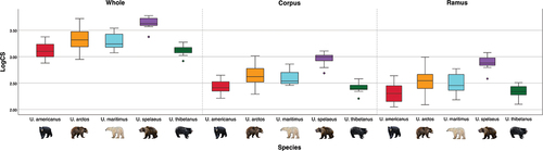
A large portion of variation in each dataset was due to size (40.5%, 59.9%, and 39.4% for whole mandible, corpus and ramus datasets, respectively) with the ANOVA revealing statistically significant species size differences in all three datasets (p < 0.001; Table 3; Figure 4). Pairwise permutation tests between species showed statistically significant differences in size for each dataset and resulted in p < 0.001 for all comparisons between U. spelaeus and every extant species (Table 4). When U. spelaeus is separated by stratigraphic unit, only Unit 3 specimens are significantly different in all cases (Table 4). Across all datasets, all pairwise comparisons between U. arctos and U. maritimus, plus U. americanus and U. thibetanus returned non-statistically significant results (Table 4). There is a significant allometric signal on shape across species for whole mandible, corpus and ramus datasets although it explains a small proportion of variance (between 3% and 9%) and allometric trajectories do not differ between species (p > 0.200, Table 3).

Figure 4. Boxplots showing differences in log centroid size (logCS) of whole mandible, corpus and ramus specimens across all species of Ursus.

Ecogeographical variation

Partial least squares analyses show strong covariation between mandible shape and the selected bioclimatic variables (16 for whole mandible, 15 for corpus and 12 for ramus; Table S3), with the first pair of PLS axes explaining 88.73%, 95.95% and 76.91%; and the second pair of PLS axes explaining 8.28%, 3.30% and 17.03% of covariation for whole mandible, corpus and ramus datasets, respectively (Figures 5 and 6). The climatic variables that showed a significant correlation with ursid mandible shape were: i) whole mandible, Bio 1–13, 15–16, 18; ii) corpus Bio 1, 3–13, 15–16, 18; iii) ramus Bio 1–3, 5–6, 8–11, 17–19 (Table S3). All PLS1 and PLS2 for whole mandible, corpus and ramus datasets were statistically significant (p < 0.01). The correlations between shape PLS1 and climate PLS1 for all datasets (whole mandible, corpus and ramus) were high and significant (whole mandible: r = 0.766, p < 0.001, Figures 5A–D and 6A–D; corpus: r = 0.712, p < 0.001, Figures 5B–E and 6B–E; ramus: r = 0.553, p < 0.001, Figures 5C–F and 6C–F). This shows bears that inhabit colder, drier and more seasonal environments have a more slender mandible shape with a relatively dorsoventrally thinner corpus and ramus, a straighter corpus body and a larger diastema. Bears from these climates also show a dorsoventrally smaller ramus, differentiating from specimens with a taller ramus that inhabit warmer, less seasonable environments with higher levels of precipitation.

Figure 5. Scatterplot of the first pair of PLS of shape and climate by: species (a, b and c) and Köppen-Geiger climate classification (d, e and f) for whole mandible (a and d), corpus (b and e) and ramus (c and f) datasets. Deformation grids and two-coloured wireframes show mean shape (light blue) and deformation (dark blue) at the extremity of the first axis. All stratigraphic unit specimens = U. spelaeus.

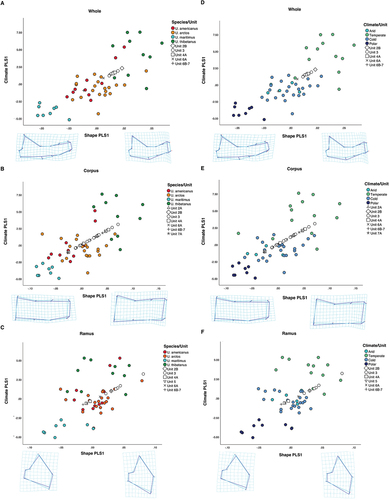
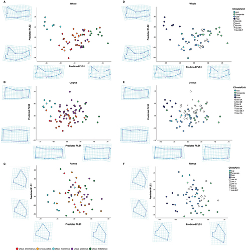
Figure 6. Scatterplot of the predicted PLS scores of shape by: species (a, b and c) and Köppen-Geiger climate classification (d, e and f) for whole mandible (a and d), corpus (b and e) and ramus (c and f) datasets. Deformation grids and two-coloured wireframes show mean shape (light blue) and deformation (dark blue) at the extremities of both x and y axes. All stratigraphic unit specimens = U. spelaeus.

Partial least square plots of the whole mandible show the polar bear (U. maritimus) occupying mainly negative scores (Figures 5 and 6), while the Asian black bear (U. thibetanus) scores positively with small overlap with specimens of U. arctos and U. americanus from warmer, less seasonal areas. These morphological differences are also present in bears of the same species that inhabit different environments. Specimens of U. arctos and U. americanus located in colder, more seasonal environments such as Alaska and Canada show morphological shape that clusters closer to specimens of U. maritimus (Figures 5 and 6), while specimens of these species from warmer habitats with higher precipitation show morphology closer to specimens of U. thibetanus.

The cave bear (U. spelaeus) occupies a range of scores in shape space (Figures 5 and 6), clustering with specimens of U. americanus, U. arctos and U. thibetanus. The PLS scatter plot for the ramus dataset (Figure 6c) shows greater overlap than whole mandible and corpus datasets (Figure 6(A,B), respectively). This is also the case in Köppen-Geiger climate classification scatter plots (Figure 6D–F). Parametric MANOVA of PLS1 and PLS2 based on Köppen-Geiger climate classifications showed statistically significant difference in shape for all datasets; whole mandible: F _{(6, 86)} = 28.247, p < 0.001, Wilks’ λ = 0.113, partial η² = 0.663; corpus F _{(6, 88)} = 13.492, p < 0.001, Wilks’ λ = 0.271, partial η² = 0.479; ramus: F _{(6, 86)} = 6.786, p < 0.001, Wilks’ λ = 0.461, partial η² = 0.321. p values were further confirmed by NPMANOVA (p < 0.001 in all cases). Köppen-Geiger plots identify a degree of discrimination between climatic groups based on shape (whole mandible and corpus datasets) with cold, dry and less seasonal environments clustering in a negative PLS1 shape space while warmer, more seasonal environments with higher precipitation scoring more positively, Figures 6D,E. Warmer and more temperate scores for extant bears share shape space with cave bears from stratigraphic units 2B and 4A (Figure 6D).

Cave bear specimens from Units 2B and 4A cluster with temperate species, comprising U. thibetanus, U. arctos and U. americanus, on PLS1 while specimens from sedimentary units 6B–7 show negative scores in shape space, closer to the polar bear. In sedimentary units for the corpus dataset (Figure 6E), cave bears show large overlap with the majority of specimens scoring positively in PLS1 and PLS2. Unit 3 specimens are widespread in the PLS shape space, while unit 7A specimens exhibit negative PLS2 scores clustering close to U. thibetanus, due to a relatively thicker corpus body in comparison to mean shape. Köppen-Geiger plots for ramus show a spread of morphology when categorised by climate in both extant and extinct specimens. As with the corpus (Figure 6E), unit 3 specimens span shape space, here in PLS2 of ramus specimens (Figure 6F) while scoring completely in positive PLS1 (relating to a relatively taller/thinner ramus shape). Colder related units congregate around the central region of the PLS space.

Discriminant function analyses on extant species identified a high percentage of correctly classified cases for specimens of polar climates (>75.00%) in all datasets, confirming their distinctiveness compared to other climate types (Table 6). Cold climate classification shows the lowest percentage accuracy of correct classification across all datasets (Table 6), with many of these specimens being classified to arid climate class and vice versa.

Table 5. Summary of variation by the first two axes of DFAs on the Whole mandible, Corpus and Ramus datasets. Significance indicated in bold.

		Wilks’ λ	x^2	df	P	% of var
Whole	DF1	0.126	91.153	6	<0.001	82.3%
	DF2	0.569	24.784	2	<0.001	17.7%
Corpus	DF1	0.281	57.044	6	<0.001	78.4%
	DF2	0.706	15.669	2	<0.001	21.6%
Ramus	DF1	0.439	36.198	6	<0.001	88.7%
	DF2	0.886	5.339	2	0.069	11.3%

Table 6. Percentage of cross-validated correctly classified cases of each climate classification for discriminant function analysis for each dataset (whole mandible, corpus and ramus) on extant bear species. Percentages of correctly classified cases are in bold.

		Arid	Temperate	Cold	Polar
Whole	Arid	40.00%	0.00%	60.00%	0.00%
	Temperate	0.00%	83.3%	16.7%	0.00%
	Cold	43.50%	13.00%	43.5%	0.00%
	Polar	12.50%	0.00%	0.00%	87.50%
Corpus	Arid	60.00%	0.00%	40.00%	0.00%
	Temperate	7.70%	69.20%	15.40%	7.70%
	Cold	34.80%	30.40%	34.80%	0.00%
	Polar	12.50%	0.00%	0.00%	87.50%
Ramus	Arid	20.00%	20.00%	60.00%	0.00%
	Temperate	16.70%	66.70%	8.30%	8.30%
	Cold	39.10%	21.70%	26.10%	13.00%
	Polar	12.50%	0.00%	12.50%	75.00%

Discriminant function analyses were computed on all three datasets (whole mandible, corpus and ramus) using significant allometrically corrected PLS1 and PLS2 morphology vector scores for cave bear specimens. For the whole mandible and corpus datasets, discriminant functions DF1 and DF2 were found to be statistically significant (Table 5). The DFA on the ramus dataset gave different results, with only DF1 found to be statistically significant (Table 5). DFA further predicted climatic group membership for specimens of U. spelaeus in stratigraphic groups across all datasets based on shape (Table 7). Climate predictions of U. spelaeus using DFA shows varied climatic conditions across all units in all datasets with regard to shape (Table 7). The corpus dataset provides the most variation in climatic conditions, with multiple climate classifications for specimens from single stratigraphic units. Unit 3 shows the largest variation of predicted climates, ranging from polar to temperate environments (Table 7).

Table 7. Predicted Köppen-Geiger climate classifications for U. spelaeus specimens from different stratigraphic units of Scladina Cave for shape in each dataset (whole mandible, corpus and ramus) based on DFA models.

		DFA Predicted Climate Group
Specimen No	Unit	Whole	Corpus	Ramus
SC 91–509	2A	-	Temperate*	-
SC 02-787-3	2A	-	Arid*	-
SC 03-68-9	2B	Temperate*	Temperate*	Temperate*
SC 83-99-2	3	-	Temperate*	-
SC 87–3	3	-	Temperate*	-
SC 91-582-15	3	Cold	Arid*	Temperate*
SC 91-582-75	3	-	Polar	-
SC 92-113-32	3	-	Temperate*	-
SC 92-1280-01	3	-	Temperate*	-
SC 92-502-21	3	-	Temperate*	-
SC 92-503-01	3	Cold	Arid	Temperate*
SC 92-507-7	3	Cold	Arid	Temperate*
SC 93-24-78	3	-	Cold	-
SC 93-30-34	3	-	Arid	-
SC 94	3	-	Polar	-
SC 98-178-293	3	Polar	Temperate*	Temperate*
SC 98-275-198	3	-	Cold	-
SC 03–566	3	-	Temperate*	-
SC 04-221-5	3	Cold	Temperate*	Temperate*
SC 87-90-40	5	-	-	Temperate*
SC 82-81-3129	4A	-	Polar	-
SC 83-109-2274	4A	Temperate*	Temperate*	Arid
SC 90-95-2278	4A	-	Temperate*	-
SC 93-109-2874	4A	Temperate*	Temperate*	Arid
SC 98–235	6A	-	Polar	-
SC 04-578-17	6A	-	Arid	-
SC 04-578-18	6A	-	Temperate	-
SC 04-578-21	6A	-	Arid	-
SC 04-578-26	6A	Cold*	Polar	Cold*
SC 05-498-1	6A	-	-	Cold*
SC 13-175-1	6B–7	Arid*	Arid*	Cold
SC 13-356-2	6B–7	-	Temperate	-
SC 02-52-1	7A	-	Cold*	-

*Denotes the most common prediction for that Unit.

Discussion

For the first time, extant skeletal morphology and bioclimatic variables have been utilised to predict palaeoclimates of Ursus spelaeus through a single sites stratigraphic chronology. We find that mandibular morphology is distinctive among bear species and appears to be indirectly linked to climate, a pattern demonstrated both within and between species. This concurs with a previous study (Meloro et al. 2017). We also show that the cave bear exhibits a distinct mandibular morphology, that changes through stratigraphic units, compared to that of extant bear species and highlights the potential impact environmental differences have on trophic diversity. Similar results have been obtained previously for mandible shape (e.g. Fuchs et al. 2015; van Heteren et al. 2016) which suggest that mandibular morphologies strongly reflect diet. Hence, the disparity between extant bear species and the cave bear seem to be characterised by distinctive adaptations for herbivory in the latter (van Heteren et al. 2019).

We identify a degree of taxonomic discrimination when looking at the corpus and ramus separately. Interestingly, the corpus seems to show a stronger taxonomic signal in Ursus species. This is not surprising considering that the corpus houses the dentition: the number, positions and morphology are known to be highly informative in other groups such as the Carnivora (Meloro et al. 2008, 2011). Previous studies confirmed this at an interspecific scale, suggesting modifications of the mandibular corpus of cave bears and other species of Ursidae in relation to dental apparatus; with the cave bear expressing an elongated corpus allowing room for dental modifications in M₃ (van Heteren et al. 2009, 2014, 2016; Meloro et al. 2011). Similarly in the cranium, modifications to the paranasal sinuses compromised biomechanical performance of the skull, causing a domed forehead (typical of speloid bears) that reduces the dissipation of bite stress. This modification would have forced cave bears to have a skull morphologically constrained to masticating vegetation with the posterior dentition (Pérez-Ramos et al. 2020). Further to this, modifications in M₃ itself of U. spelaeus also validate this point, showing different evolutionary shape trajectories than other dentition in the tooth row relating to a size increase of the talonid grinding platform through time, to aid in the processing and consumption of low-quality plant material (Charters et al. 2022).

There are large size contrasts between bear taxa, with cave bears being exceptionally large compared to all the other extant species in the genus (Figures 3, 4 and Table 4). However, variation between stratigraphic unit specimens of U. spelaeus is a different case, showing non-statistical differences in size between any units (Table 4). The size difference shown by U. spelaeus may be due to a level of niche partitioning. Cave bears and brown bears lived in sympatry during the Pleistocene and have been found to express different diets (more herbivorous and omnivorous, respectively) through isotope analyses, suggesting ecological competition between these species was likely limited and further expressing the degree of dietary flexibility brown bears had already developed in late Pleistocene Europe (Bocherens et al. 2011). Similarly, during the late Pleistocene in North America, brown bears coexisted with the giant short-faced bear Arctodus simus. Isotope analyses suggested that while coexisting with this specialised carnivore, brown bears were mainly herbivorous until the extinction of A. simus (Barnes et al. 2002), with a potentially similar case of dietary variation between herbivorous cave bears and predominantly meat consuming brown bears, already suggested for individuals of Scladina Cave (Bocherens and Drucker 2006).

The shape of the mandible of U. spelaeus is characterised by a thick curved corpus tall ramus and largely developed diastema, similar to that of U. arctos. Shape variation of the cave bear shows overlap with some species of Ursus, with cave bears showing similar morphologies to U. americanus, U. arctos and U. thibetanus.

Bear specimens that show a slender mandible shape, with a relatively longer thinner corpus body, dorsoventrally smaller ramus and a large diastema are associated with cold, highly seasonal environments whereas bears with a mandible shape of a relatively shorter, thicker more curved corpus, smaller diastema and taller, antero-posteriorly thinner ramus occupy generally warmer regions with higher precipitation. Cold and Arid climate classifications showed the lowest percentage of correct climate classification, with specimens often being classified as relating to each other environments. This may be due to the mutual exclusive nature of Temperate, Cold, and Polar classes, were the non-mutually exclusive Arid climate class may intersect other climate classifications (Beck et al. 2018).

Other factors such as intraspecific variation and topography may also cause mandibular divergence. Sedimentary dynamics and intra-unit complexity also probably played a role, especially in complex units such as 4A and 3 (see Pirson et al. 2014). Multiple sub-species of U. arctos are in our sample (U. a. alascensis, U. a. gyas, U. a. isabellinus (recorded inhabiting high altitudes in the Himalayas, Sharief et al. 2020), U. a. dalli, U. a. horribillis, U. a. marsicanus, U. a. middendorfi, U. a. arctos) that inhabit different points on a vast ecological gradient (Krechmar 1995), being morphologically distinct. Previously noted by Meloro et al. (2017), sub-species of U. arctos show large variation in correctly classified cases (50%–100%). Isotopic evidence has pointed to an association between altitude related climatic variation and diet, with high altitude precipitation (snowfall) having a greater impact on meat consumption in U. arctos than at lower altitudes (García‐Vázquez et al. 2023. Similarly in cave bears, a decreasing δ¹⁵N signature is found along altitudinal gradients (Krajcarz et al. 2016), reflecting known altitude gradients for modern plant species (Männel et al. 2007).

The cave bear specimens used in this study correspond to multiple climate classifications associated with stratigraphic units in the Scladina Cave. Unit 2A specimens were likely to correspond to arid climates in-line with the palynology of the unit which showed dominance of herb pollen and presence of steppe taxa that together indicate cold dry conditions (Pirson et al. 2008). Unit 2A has been previously suggested as a MIS 4 deposit which is supported here, however a temperate classification suggests specimens may be from early MIS 4, further suggested from low Green Amphibole concentrations in the silt fraction (Pirson et al. 2014). Unit 2A may however indicate reworking of the underlying temperate Unit 2B, instead of a separate chronoclimatic signal.

Temperate climate classification for U. spelaeus specimens from units 2B across all datasets cluster on the boundary of extant cold and temperate specimens in PLS shape space. This suggests climatic improvement, supported by high percentage of tree pollen (mainly Picea and Pinus) and fern spores throughout the unit and previously interpreted to reflect more humid local conditions (Pirson et al. 2008). Anthracological data from this unit further supports a temperate boreal environment with high amounts of Pinus and Picea found in charcoal remains (Pirson et al. 2008, 2014).

Unit 3 appeared to have a variable climate. In whole mandible shape space, a cold climate is inferred, while for ramus, a temperate climate appears more likely. The corpus dataset predict cave bear in all climate classifications (Temperate, Arid, Cold and Polar) with specimens possibly representing the climatic fluctuation of different MIS sub-stages within MIS 5 (Lambeck et al. 2002). Pirson et al. (2008) previously suggested a contrasted environment ranging from open steppe to forest steppe, with low pollen concentration within layers of the unit, dominated by herbs, forbs and low percentages of boreal tree pollen. However, climatic fluctuation has been previously suggested in Unit 3 (analysed with clear distinction between layers within the unit) with stalagmitic floors being found overlaying Units 3 INF and 3 SUP, indicating contrasting climates with at least one colder and two warmer periods within Unit 3 (Pirson et al. 2014). The large variation of specimens within the unit in shape and known climatic fluctuation in MIS 5 May further show shifts in diet, reflected in the corpus due to morphological adaptation in dentition.

Within Unit 4A, the majority of specimens appear to be related to a temperate environment. Our findings agree with suggestions of climatic improvement within the unit, supported by palynology with the presence of conifer, malacophyll trees, fern spores, other temperate taxa and a peak in algae (Pirson et al. 2014). This is further supported by a thick stalagmitic floor within the unit, indicative of climatic improvement (Quinif et al. 1994). A large climatic fluctuation in Unit 4A suggests a range of climates for specimens found in this unit. Similar to that of Unit 3, multiple climate predictions for this unit may be due to its composition of numerous sedimentary layers reflecting climate transitions and sediment reworking within, from a temperate to a boreal environment suggested from pollen spectra (Pirson et al. 2008), possibly associated to a series of MIS 5 sub-stages in early MIS 5.

Unit 5 is suggested as showing clear signs of climatic cooling or a possible steppe environment with palynology dominated by herbs and other steppe taxa (Pirson et al. 2014). However, the presence of small mammals and large herbivorous animals show the persistence of forest taxa (Cordy 1992; Simonet 1992). The specimen of Unit 5 suggests temperate conditions, with morphology similar to that of extant bears of temperate classification. It could be possible that this specimen comes from early MIS 5, however no robust suggestions can be deduced from a small representation of the unit.

Unit 6A appears to show a cold environment, clustering close to other cold classified specimens in whole mandible and ramus datasets while like in other units, mixed environments are again suggested when corpus shape is analysed. These results support findings of the dominance of steppe herbs and lack of malacophyll trees in the unit (Pirson et al. 2008). The varying climates suggested by corpus specimens supports palynology suggesting an environment gradient through layers of unit 6A, with indications of temperate environments at the base (possibly correlated to reworking of Unit 6B), moving to a steppe environment at its top (Pirson et al. 2008).

Units 6B to 7 specimens suggest cold and arid environments, similar in morphology to specimens of U. arctos and U. americanus from cold habitats. Major climatic fluctuations have been suggested throughout these units, with strong speleothem development found in Unit 6B, while Units 6D and 6C have been suggested as climatically colder (Pirson et al. 2008) previously suggested as pertaining to MIS 5/6 (Pirson et al. 2014). Due to the lack of stratigraphic accuracy of the specimens at the time of excavation and collection (potentially relating to units 6B, 6C, 6D or 7 and further layers within these units), specific climatic interpretations for single units cannot be accurately derived.

The specimen from Unit 7A groups with extant cold/temperate specimens and were further classified as a cold environments. With cold and arid climatic predictions for Unit 6B to 7 (possibly late MIS 6/early MIS 5), Unit 7A may be related to a slightly climatically improved phase within MIS 5/6, reworked MIS 5/6, or potentially reworked sedimentary deposits from MIS 7. Previous suggestions of Unit 7A remain unclear, with clear sediment reworking found in the unit (reworked speleothem and reworked humiferous soil; Pirson 2007; Pirson et al. 2008).

Here, climate predictions are suggested using whole mandible and separated components (corpus and ramus) of U. spelaeus. However, climate predictions for the corpus dataset show large variations, with multiple climates suggested for many stratigraphic units. This demonstrates considerable morphological variation in the corpus of cave bears within the same stratigraphic unit in shape and an approach based on GMM also in conjunction with isotopic information (δ¹⁸O and δ¹³C) or other techniques such as dental microwear may be better suited in predicting past climates. Further, with more precise dating methods for individual stratigraphic units and accurate stratigraphic position of specimens down to single sedimentary deposits, stronger supporting arguments and more robust predictions on morphological changes relating to specific MIS stages/climatic periods can be made regarding U. spelaeus in Scladina Cave and other chronostratigraphic sedimentary sequences. This is particularly the case regarding Units 3, 4A and 6B to 7 here, with multiple stratigraphic layers within these units that suggest high climatic fluctuation.

Conclusion

Here, we show that climate has an impact on the functional morphology of the mandible in extant and extinct bear species. Species of Ursus can also be discriminated through the use of 2D GMM. The mandibles of bears that inhabit cold, dry, seasonal environments have a slender morphology possessing a straighter, flatter corpus and a larger diastema relative to bears from less seasonal, warmer environments with higher rates of precipitation. Bears from warmer environments are found to have a shorter, thicker corpus that is more curved with a smaller diastema. This is found inter and intraspecifically. A series of climatic classifications were suggested to aid in the assessment of previously suggested Marine Isotope Stages for specimens related to sedimentary deposits in Scladina Cave. Through the broad ecogeographic and dietary variation within and between species of extant Ursus, suggestions on palaeoclimate can be made for the extinct species U. spelaeus. Using related faunal remains from associated stratigraphic sedimentary units is a first step in adding to the understanding of cave sediment chronology and their climates. These results could be refined by taking into account a larger representative sample for each unit and a vastly more detailed stratigraphic attribution in the future. Techniques used here could be further applied to other genera to interpret feeding ecology and palaeoenvironments.

Acknowledgments

The authors are extremely grateful to the curators of collections for access to the specimens used herein particularly: E. Westwig (American Museum of Natural History, New York, USA); L. Rook and E. Cioppi (Museo Di Geologia e Paleontologia, Università di Firenze, Italy); S. Fraile Gracia (Museo Nacional De Ciencias Naturales, Madrid, Spain); P. Agnelli (Museo Zoologico ‘La Specola’ Firenze, Italy); P. Jenkins, L. Tomsett, R. Portela-Miguez, A. Salvador, D. Hills (Natural History Museum Of London, UK) and T. Parker (World Museum Liverpool, Liverpool, UK). P. Colangelo and G. Guidarelli also kindly helped sharing their database of bear images. The authors further thank D. Bonjean for the help with improving this manuscript and for the continued dedication to the Scladina project. D. Charters is very grateful for the continued support from family and friends during this project. We also express our thanks to three anonymous reviewers for their valuable comments.

Disclosure statement

No potential conflict of interest was reported by the author(s).

Supplementary material

Supplemental data for this article can be accessed online at https://doi.org/10.1080/08912963.2024.2377703.

Additional information

Funding

D. Charters research visit to Madrid, Spain, was financially supported by SYNTHESYS+ H2020 project [ES-TAF-2882]: Ecomorphological evolution of cave and brown bears across the European Quaternary.

References

- Adams DC, Collyer ML. 2015. Permutation tests for phylogenetic comparative analyses of high-dimensional shape data: what you shuffle matters. Evolution. 69(3):823–829. doi: 10.1111/evo.12596.
- Adams D, Collyer M, Kaliontzopoulou A, Baken E. 2022. Geomorph: Software for geometric morphometric analyses. R package version 4.0.4. https://cran.r-project.org/package=geomorph.
- Adams DC, Otárola-Castillo E, Paradis E. 2013. Geomorph: an R package for the collection and analysis of geometric morphometric shape data. Meth Ecol Evol. 4(4):393–399. doi: 10.1111/2041-210X.12035.
- Adams DC, Rohlf FJ, Slice DE. 2004. Geometric morphometrics: Ten years of progress following the ‘revolution’. Italian J Zool. 71(1):5–16. doi: 10.1080/11250000409356545.
- Azzaroli A. 1983. Quaternary mammals and the Bend-Villafranchian dispersal event - a turning point in the history of Eurasia. Palaeogeogr, Palaeoclimatol, Palaeoecol. 44(1–2):117–139. doi: 10.1016/0031-0182(83)90008-1.
- Baken EK, Collyer ML, Kaliontzopoulou A, Adams DC. 2021. gmShiny and geomorph v4.0: new graphical interface and enhanced analytics for a comprehensive morphometric experience. Methods Ecol Evol. 12(12):2355–2363. doi: 10.1111/2041-210X.13723.
- Barnes I, Matheus P, Shapiro B, Jensen D, Cooper A. 2002. Dynamics of pleistocene population extinctions in beringian brown bears. Science. 295(5563):2267–2270. doi: 10.1126/science.1067814.
- Baryshnikov G. 2007. Bears Family (Carnivora, Ursidae). Nauka, St. Petersburg (Fauna of Russia and Neighboring Countries, new series 147) (in Russian).
- Baryshnikov GF, Puzachenko AY. 2011. Craniometrical variability of cave bears (Carnivora, Ursidae): multivariate comparative analysis. Quaternary Int. 245(2):350–368. doi: 10.1016/j.quaint.2011.02.035.
- Baryshnikov G, Lavrov AV. 2013. Pliocene bear Ursus minimus Devèze de Chabriol et Bouillet, 1827 (Carnivora, Ursidae) in Russia and Kazakhstan. Russ J Theriol. 12(2):107–118. doi: 10.15298/rusjtheriol.12.2.07.
- Bastin B. 1992. Analyse pollinique des sèdiments détritiques, des coprolithes et des concrétions stalagmitiques du site préhistorique de la grotte Scladina (Province de Namur, Belgique). In: Otte M, editor. Recherches aux grottes de Sclayn, Volume 1: Le contexte. Études et Recherches Archéologiques de l’Université de Liège Vol. 27. Belgium: ERAUL; p. 59–77.
- Beck H, Zimmermann N, McVicar T, Vergopolan N, Berg A, Wood EF. 2018. Present and future Köppen-Geiger climate classification maps at 1-km resolution. Sci Data. 5(1):180214. doi: 10.1038/sdata.2018.214.
- Blain HA, López-García JM, Cordy JM, Pirson S, Abrams G, Di Modica K, Bonjean D. 2014. Middle to Late Pleistocene herpetofauna from Scladina and Sous-Saint-Paul caves (Namur, Belgium). Comptes Rendus Palevol. 13(8):681–690.
- Bocherens H. 2015. Isotopic tracking of large carnivore palaeoecology in the mammoth steppe. Quaternary Sci Rev. 117:42–71. doi: 10.1016/j.quascirev.2015.03.018.
- Bocherens H. 2019. Isotopic insights on cave bear palaeodiet. Historical Biol. 31(4):410–421. doi: 10.1080/08912963.2018.1465419.
- Bocherens H, Baryshnikov G, van Neer W. 2014. Were bears or lions involved in salmon accumulation in the Middle Palaeolithic of the Caucasus? An isotopic investigation in Kudaro 3. Quaternary Int. 339– 340:112–118. doi: 10.1016/j.quaint.2013.06.026.
- Bocherens H, Billiou D, Patou-Mathis M, Bonjean D, Otte M, Mariotti A. 1997. Paleobiological implications of the isotopic signatures (13C, 15N) of fossil mammal collagen in Scladina Cave (Sclayn, Belgium). Quat Res. 48(3):370–380. doi: 10.1006/qres.1997.1927.
- Bocherens H, Drucker D. 2006. Dietary competition between Neanderthals and Modern Humans: insights from stable isotopes. In: Conard N, editor. Neanderthals and Modern Humans Meet? Tübingen: Kerns Verlag; p. 129e143.
- Bocherens H, Drucker DG, Billiou D, Geneste JM, van der Plicht J. 2006. Bears and humans in Chauvet Cave (Vallon-Pont-d’Arc, Ardèche, France): Insights from stable isotopes and radiocarbon dating of bone collagen. J Hum Evol. 50(3):370–376. doi: 10.1016/j.jhevol.2005.12.002.
- Bocherens H, Stiller M, Hobson KA, Pacher M, Rabeder G, Burns JA, Tütken T, Hofreiter M. 2011. Niche partitioning between two sympatric genetically distinct cave bears (Ursus spelaeus and Ursus ingressus) and brown bear (Ursus arctos) from Austria: isotopic evidence from fossil bones. Quat Int. 245(2):238–248. doi: 10.1016/j.quaint.2010.12.020.
- Bon C, Caudy N, de Dieuleveult M, Fosse P, Philippe M, Maksud F, Beraud-Colomb É, Bouzaid E, Kefi R, Laugier C, et al. 2008. Deciphering the complete mitochondrial genome and phylogeny of the extinct cave bear in the Paleolithic painted cave of Chauvet. Proc Natl Acad Sci USA. 105(45):17447–17452. doi: 10.1073/pnas.0806143105.
- Bookstein F. 1991. Morphometric tools for landmark data: geometry and biology. Cambridge (UK); New York: Cambridge University Press.
- Bookstein F. 1996. Biometrics, biomathematics and the morphometric synthesis. Bull Math Biol. 58(2):313–365. doi: 10.1007/BF02458311.
- Cáceres N, Meloro C, Carotenuto F, Passaro F, Sponchiado J, Melo GL, Raia P, Riddle B. 2014. Ecogeographical variation in skull shape of capuchin monkeys. J Biogeogr. 41(3):501–512. doi: 10.1111/jbi.12203.
- Charters D, Abrams G, De Groote I, Di Modica K, Bonjean D, Meloro C. 2019. Temporal variation in cave bear (Ursus spelaeus) dentition: The stratigraphic sequence of Scladina Cave. Belgium Quaternary Sci Rev. 205:76–85. doi: 10.1016/j.quascirev.2018.12.012.
- Charters D, Brown RP, Abrams G, Bonjean D, De Groote I, Meloro C. 2022. Morphological evolution of the cave bear (Ursus spelaeus) mandibular molars: coordinated size and shape changes through the Scladina Cave chronostratigraphy. Palaeogeogr, Palaeoclimatol, Palaeoecol. 587:110787. doi: 10.1016/j.palaeo.2021.110787.
- Collyer ML, Adams DC. 2018. RRPP: RRPP: An R package for fitting linear models to high-dimensional data using residual randomization. Methods Ecol Evol. 9(2):1772–1779. doi: 10.1111/2041-210X.13029.
- Collyer ML, Adams DC. 2019. RRPP: Linear Model Evaluation with Randomized Residuals in a Permutation Procedure. https://CRAN.R-project.org/package=RRPP.
- Collyer ML, Adams DC. 2021. RRPP: Linear Model Evaluation with Randomized Residuals in a Permutation Procedure. https://cran.r-project.org/web/packages/RRPP.
- Collyer ML, Sekora DJ, Adams DC. 2015. A method for analysis of phenotypic change for phenotypes described by high-dimensional data. Heredity (Edinb). 115(4):357–365. doi: 10.1038/hdy.2014.75.
- Cordy JM. 1992. Bio- et chronostratigraphie des dépôts quaternaires de la grotte Scladina (province de Namur, Belgique) à partir des micromammifères. In: Otte M, editor. Recherches aux grottes de Sclayn Volume 1: Le contexte. Études et Recherches Archéologiques de l’Université de Liège Vol. 27. Belgium: ERAUL; p. 79–125.
- Croizet A, Jobert A. 1828. Recherches Sur Les Ossemens Fossils du Département du Puy-de-Dôme 224. Paris: Chez les Princip. Library.
- Cuvier G. 1823. Recherches sur les ossemens fossiles, où l’on rétablit les caractères de plusieurs animaux dont les révolutions du globe ont détruits les espèces. T.4. Paris: Chez G. Dufour et E. D’Ocagne, Libraires, et a Amsterdam, chez les mèmes (in French).
- Dabney J, Knapp M, Glocke I, Gansauge MT, Weihmann A, Nickel B, Valdiosera C, García N, Pääbo S, Arsuaga J-L, et al. 2013. Complete mitochondrial genome sequence of a Middle Pleistocene cave bear reconstructed from ultrashort DNA fragments. PNAS. 110:15758–15763.
- Devèze de Chabriol JS, Bouillet, JB.1827. Essai géologique et minéralogique sur les environs d’lssoire, department du Puy-de-Dôme, et principalement sur la montagne de Boulade, avec la description et des figures lithographiées des ossemens fossils qui ont été recueillis. France: Clermont-Ferrand.
- Fick SE, Hijmans RJ. 2017. WorldClim 2: new 1-km spatial resolution climate surfaces for global land areas. Intl J Climatol. 37(12):4302–4315. doi: 10.1002/joc.5086.
- Figueirido B, Palmqvist P, Pérez-Claros JA. 2009. Ecomorphological correlates of craniodental variation in bears and paleobiological implications for extinct taxa: an approach based on geometric morphometrics. J Zool. 277(1):70–80. doi: 10.1111/j.1469-7998.2008.00511.x.
- Fuchs M, Geiger M, Stange M, Sánchez-Villagra MR. 2015. Growth trajectories in the cave bear and its extant relatives: an examination of ontogenetic patterns in phylogeny. BMC Evol Biol. 15(1):239. doi: 10.1186/s12862-015-0521-z.
- Funk C, Verdin A, Michaelsen J, Peterson P, Pedreros D, Husak G. 2015. A global satellite-assisted precipitation climatology. Earth Syst Sci Data. 7(2):275–287. doi: 10.5194/essd-7-275-2015.
- García‐Vázquez A, Crampton DA, Lamb AL, Wolff GA, Loy G, Guidarelli A, Groff P, Ciucci C, Pinto‐Llona AC, Grandal‐d’Anglade A, et al. 2023. Isotopic signature in isolated south‐western populations of European brown bear (Ursus arctos). Mamm Res. 68(1):63–76. doi: 10.1007/s13364-022-00654-2.
- Garsia N. 2003. Osos y otros carnivoros de la Sierra de Atapuerca. Spain: Fundacion Oso de Asturias.
- Gower J. 1975. Generalized Procrustes analysis. Pyschometrika. 40(1):33–51. doi: 10.1007/BF02291478.
- Haesaerts P. 1992. Les dépôts pléistocènes de la terrasse de la grotte Scladina à Sclayn (province de Namur, Belgique). In: Otte M, editor. Recherches aux grottes de Sclayn Volume 1: Le contexte. Études et Recherches Archéologiques de l’Université de Liège Vol. 27. Belgium: ERAUL; p. 33–55.
- Hailer F, Kutschera VE, Hallström BM, Klassert D, Fain SR, Leonard JA, Arnason U, Janke A. 2012. Nuclear genomic sequences reveal that polar bears are an old and distinct bear lineage. Science. 336(6079):344–347. doi: 10.1126/science.1216424.
- Hänni C, Laudet V, Stehelin D, Taberlet P. 1994. Tracking the origins of the cave bear (Ursus spelaeus) by mitochondrial DNA sequencing. Proc Natl Acad Sci USA. 91(25):12336–12340. doi: 10.1073/pnas.91.25.12336.
- Hijmans RJ, Cameron SE, Parra JL, Jones PG, Jarvis A. 2005. Very high resolution interpolated climate surfaces for global land areas. Int J Climatol. 25(15):1965–1978. doi: 10.1002/joc.1276.
- Hijmans RJ, Guarino L, Cruz M, Rojas E. 2001. Computer tools for spatial analysis of plant genetic resources data: 1. DIVA-GIS. Plant Genetic Resour Newsl. 127:15–19.
- Hijmans RJ, Guarino L, Mathur P. 2012. DIVA-GIS Version 7.5 Manual. https://diva-gis.org/.
- Karger DN, Conrad O, Böhner J, Kawohl T, Kreft H, Soria-Auza RW, Zimmermann NE, Linder HP, Kessler M. 2017. Climatologies at high resolution for the earth’s land surface areas. Sci Data. 4(1):170122. doi: 10.1038/sdata.2017.122.
- Klingenberg CP. 2011. MorphoJ: an integrated software package for geometric morphometrics. Mol Ecol Resour. 11(2):353–357. doi: 10.1111/j.1755-0998.2010.02924.x.
- Klingenberg CP. 2013. Visualizations in geometric morphometrics: how to read and how to make graphs showing shape changes. Hystrix. 24(1):15–24.
- Knapp M, Rohland N, Weinstock J, Baryshnikov G, Sher A, Doris N, Rabeder G, Pinhasi R, Schmitt H, Hoffreiter M. 2009. Fist DNA sequences of Asian cave bear fossils reveal deep divergences and complex phylogeographic patterns. Mol Ecol. 18(6):1225–1238. doi: 10.1111/j.1365-294X.2009.04088.x.
- Köppen W. 1936. Das geographisca System der Klimate. In: Köppen W. and Geiger GC, and Gebr B, editors. Handbuch der Klimatologie. Berlin: Borntraeger; p. 1–44.
- Krajcarz MP, Krajcarz MT, Laughlan L, Rabeder G, Sabol M, Wojtal P, Bocherens H. 2016. Isotopic variability of cave bears (δ15N, δ13C) across Europe during MIS 3. Quat Sci Rev. 131:51. doi: 10.1016/j.quascirev.2015.10.028.
- Krechmar MA. 1995. Geographical aspects of the feeding of the brown bear (Ursus arctos L.) in the extreme northeast of Siberia. Russ J Ecol. 26:436–443.
- Kumar V, Lammers F, Bidon T, Pfenninger M, Kolter L, Nilsson MA, Janke A. 2017. The evolutionary history of bears is characterized by gene flow across species. Sci Rep. 7(1):46487. doi: 10.1038/srep46487.
- Kurtén B. 1968. Pleistocene Mammals of Europe 317. London: Weidenfeld and Nicolson.
- Lambeck K, Esat T, Potter EK. 2002. Links between climate and sea levels for the past three million years. Nature. 419(6903):199–206. doi: 10.1038/nature01089.
- Linnaeus C. 1758. Systema Naturae per Regna Tria Naturae, Secundum Classes, Ordines, Genera, Species, cum Characteribus, Differentiis, Synonymis, Locis. Editio Decima. 1:1–824.
- Liu S, Lorenzen ED, Fumagalli M, Li B, Harris K, Xiong Z, Zhou L, Korneliussen TS, Somel M, Babbitt C, et al. 2014. Population genomics reveal recent speciation and rapid evolutionary adaptation in polar bears. Cell. 157(4):785–794. doi: 10.1016/j.cell.2014.03.054.
- López-García JM, Blain HA, Cordy JM, Pirson S, Abrams G, Di Modica K, Bonjean D. 2017. Palaeoenvironmental and palaeoclimatic reconstruction of the Middle to Late Pleistocene sequence of Scladina Cave (Namur, Belgium) using the small mammal assemblages. Historical Biol. 29(8):1125–1142. doi: 10.1080/08912963.2017.1288229.
- Loreille O, Orlando L, Patou-Mathis M, Philippe M, Taberlet P, Hänni C. 2001. Ancient DNA analysis reveals divergence of the cave bear, Ursus spelaeus, and brown bear, Ursus arctos, lineages. Curr Biol. 11(3):200–203. doi: 10.1016/S0960-9822(01)00046-X.
- Männel TT, Auerswald K, Schnyder H. 2007. Altitudinal gradients of grassland carbon and nitrogen isotope composition are recorded in the hair of grazers. Glob Ecol Biog. 16(5):583–592. doi: 10.1111/j.1466-8238.2007.00322.x.
- Martin LD. 1989. Fossil history of the terrestrial Carnivora. In: Gittleman JL, editor. Carnivore behaviour, ecology and evolution. London: Chapman and Hall; p. 536–568.
- McLellan B, Reiner DC. 1994. A review of bear evolution. Bears: Their Biol Manag. 9:85–96. doi: 10.2307/3872687.
- Meloro C. 2011. Feeding habits of Plio-Pleistocene large carnivores as revealed by the mandibular geometry. J Vertebr Paleontol. 31(2):428–446. doi: 10.1080/02724634.2011.550357.
- Meloro C, Guidarelli G, Colangelo P, Ciucci P, Loy A. 2017. Mandible size and shape in extant Ursidae (Carnivora, Mammalia): A tool for taxonomy and ecogeography. J Zool Syst Evol Res. 55(4):269–287. doi: 10.1111/jzs.12171.
- Meloro C, Raia P, Carotenuto F, Cobb SN. 2011. Phylogenetic signal, function and integration in the subunits of the carnivoran mandible. Evol Biol. 38(4):465–475. doi: 10.1007/s11692-011-9135-6.
- Meloro C, Raia P, Piras P, Barbera C, O’Higgins P. 2008. The shape of the mandibular corpus in large fissiped carnivores: allometry, function and phylogeny. Zool J Linn Soc. 154(4):832–845. doi: 10.1111/j.1096-3642.2008.00429.x.
- Meloro C, Sansalone G. 2022. Palaeoecological significance of the “wolf event” as revealed by skull ecometrics of the canid guilds. Quaternary Sci Rev. 281:107419. doi: 10.1016/j.quascirev.2022.107419.
- Miller W, Schuster SC, Welch AJ, Ratan A, Bedoya-Reina OC, Zhao F, Kim HL, Burhans RC, Drautz DI, Wittekindt NE, et al. 2012. Polar and brown bear genomes reveal ancient admixture and demographic footprints of past climate change. Proc Natl Acad Sci USA. 109(36):E2382–E2390. doi: 10.1073/pnas.1210506109.
- Mitteroecker P, Gunz P. 2009. Advances in geometric morphometrics. Evol Biol. 36(2):235–247. doi: 10.1007/s11692-009-9055-x.
- Mitteroecker P, Gunz P, Windhager S, Schaefer K. 2013. A brief review of shape, form, and allometry in geometric morphometrics, with applications to human facial morphology. Hystrix, Italian J Mammal. 24(1):59–66.
- Pallas PS. 1780. Spicilegia zoologica quibus novae imprimis et obscurae animalium species iconibus, descriptionibus atque commentariis illustrantur. Fasciculus XIV. 1:1–94, Tab I-IV. Berolini.
- Pasitschniak-Arts M. 1993. Ursus arctos. Mamm Species. 439(439):1–10. doi: 10.2307/3504138.
- Peel MC, Finlayson BL, McMahon TA. 2007. Updated world map of the Köppen-Geiger climate classification. Hydrol Earth Syst Sci. 11(5):1633–1644. doi: 10.5194/hess-11-1633-2007.
- Peigné S, Goillot C, Germonpré M, Blondel C, Bignon O, Merceron G. 2009. Predormancy omnivory in European cave bears evidenced by a dental microwear analysis of Ursus spelaeus from Goyet, Belgium. Proc Natl Acad Sci USA. 106(48):15390–15393. doi: 10.1073/pnas.0907373106.
- Pérez-Ramos A, Kupczik K, Van Heteren AH, Rabeder G, Grandal-D’Anglade A, Pastor FJ, Serrano FJ, Figueirido B. 2019. A three-dimensional analysis of tooth-root morphology in living bears and implications for feeding behaviour in the extinct cave bear. Historical Biol. 31(4):461–473. doi: 10.1080/08912963.2018.1525366.
- Pérez-Ramos A, Romero A, Rodriguez E, Figueirido B. 2020. Three-dimensional dental topography and feeding ecology in the extinct cave bear. Biol. Lett. 16:20200792. doi: 10.1098/rsbl.2020.0792.
- Pérez-Ramos A, Tseng ZJ, Grandal-D’Anglade A, Rabeder G, Pastor FJ, Figueirido B. 2020. Biomechanical simulations reveal a trade-off between adaptation to glacial climate and dietary niche versatility in European cave bears. Sci Adv. 6(14):eaay9462. doi: 10.1126/sciadv.aay9462.
- Phipps CJ. 1774. A Voyage towards the North Pole undertaken by His Majesty’s command, 1773. London: Nourse.
- Pirson S. 2007. Contribution à l’étude des dépôts d’entrée de grotte en Belgique au Pléistocène supérieur. Stratigraphie, Sédimentogenèse et Paléoenvironnement [ Unpublished PhD thesis]. University of Liège and Royal Belgian Institute of Natural Sciences, vol. 1, p. 435. 5 annexes.
- Pirson S, Court-Picon M, Damblon F, Balescu S, Bonjean D, Haesaerts P. 2014. The Palaeoenvironmental context and chronostratigraphic framework of the Scladina Cave sedimentary sequence (Units 5 to 3-SUP). In: Toussaint M, and Bonjean D, editors. The Scladina I-4A Juvenile Neandertal (Andenne, Belgium), Palaeoanthropology and Context Vol. 134, Belgium: ERAUL; p. 69–92.
- Pirson S, Court-Picon M, Haesaerts P, Bonjean D, Damblon F. 2008 New data on geology, anthracology and palynology from the Scladina Cave Pleistocene sequence: preliminary results. In: Damblon F, Pirson S, Gerrienne P, editors. IVth International Meeting of Anthracology, 8–13 September, Belgium. p. 71–93.
- Quinif Y, Genty D, Maire R. 1994. Les spéléothèmes: un outil performant pour les études paléoclimatiques. Bull de la Sociétégéologique de Fr. 165:603–612.
- Rabeder G, Debeljak I, Hofreiter M, Withalm G. 2008. Morphological responses of cave bears (Ursus spelaeus group) to high-alpine habitats. Die Höhle. 4:59–72.
- Rabeder G, Hofreiter M, Nagel D, Withalm G. 2004. New taxa of alpine cave bears (Ursidae, Carnivora). In: Philippe M, Argant A, and Argant J editors. Proceedings of the 9th International Cave Bear Conference, Cahiers scientifiques du Centre de Conservation et d’Étude des Collections Museum d’Histoire naturelle de Lyon, second éd September 2003 Lyon p. 49–68.
- Rabeder G, Hofreiter M, Stiller M. 2011. Chronological and systematic position of cave bear fauna from Ajdovska jama near Krsko (Slovenia). Mitt der Kommission für Quartärforschung der Österreichischen Akad der Wissen. 20:43–50.
- Rabeder G, Pacher M, Withalm G. 2010. Early Pleistocene bear remains from Deutsch-Altenburg (Lower Austria). Mitt der Kommission für Quartärforschung der Österreichischen Akad der Wissen. 17:1–135.
- Raia P. 2004. Morphological correlates of tough food consumption in large land carnivores. Italian J Zool. 71(1):45–50. doi: 10.1080/11250000409356549.
- R Core Team. 2021. R: a language and environment for statistical computing. Vienna, Austria: R Foundation for Statistical Computing. https://www.R-project.org/.
- Reichenau WV. 1904. Über eine neue fossile Bären- Art Ursus deningeri MIHI aus den fluviatilen Sanden von Mosbach. In: Jahrb. d. nass. Ver. f. Nat Vol. 57, Wiesbaden: p. 1–11, 7.
- Rinker DC, Specian NK, Zhao S, Gibbons G. 2019. Polar bear evolution is marked by rapid changes in gene copy number in response to dietary shift. Proc Natl Acad Sci USA. 116(27):13446–13451. doi: 10.1073/pnas.1901093116.
- Rohlf FJ. 2015. The tps series of software. Hystrix, Italian J Mammol. 26:9–12.
- Rohlf FJ, Corti M, Olmstead R. 2000. Use of Two-Block Partial Least-Squares to Study Covariation in Shape. Systematic Biol. 49(4):740–753. doi: 10.1080/106351500750049806.
- Rohlf FJ, Marcus LF. 1993. A Revolution in Morphometrics. Trends Ecol Evol. 8(4):129–132. doi: 10.1016/0169-5347(93)90024-J.
- Rohlf FJ, Slice DE. 1990. Extensions of the Procrustes method for the optimal superimposition of landmarks. Syst Zool. 39(1):40–59. doi: 10.2307/2992207.
- Rosenmüller JC. 1794. Quaedam de ossibus fossilibus animalis cuiusdam, historiam eius etcognitionem accuratiorem illustrantia, dissertatio, quam d. 22. Octob. 1794 ad disputandumproposuit Ioannes Christ. Rosenmüller Heßberga-Francus, LL.AA.M. in Theatro anatomicoLipsiensi Prosector assumto socio Io. Chr. Aug. Heinroth Lips. Med. Stud. Cum tabula aenea. -34 S. Leipzig.
- Rossi M, Santi G. 2001. Archaic and recent Ursus spelaeus forms from Lombardy and Venetia Region (North Italy). Cadernos do Laboratorio Xeolóxico de Laxe. 26:317–323.
- Sharief A, Joshi BD, Kumar V, Kumar M, Dutta R, Sharma CM, Thapa A, Rana HS, Mukherjee T, Singh A, et al. 2020. Identifying Himalayan brown bear (Ursus arctos isabellinus) conservation areas in Lahaul Valley. Himachal Pradesh. 21:e00900. doi: 10.1016/j.gecco.2019.e00900.
- Simonet P. 1992. Les associations de grands mammifères du gisement de la grotte Scladina à Sclayn (Namur, Belgique). In: Otte M, editor. Recherches aux grottes de Sclayn Volume 1: Le contexte. Etudes et Recherches Archéologiques de l’Université de Liège Vol. 27. Belgium: ERAUL; p. 127–151.
- Slice DE. 2007. Geometric Morphometrics. Annu Rev Anthropol. 36(1):261–281. doi: 10.1146/annurev.anthro.34.081804.120613.
- Stiller M, Molak M, Prost S, Rabeder G, Baryshnikov G, Rosendahl W, Münzel S, Bocherens H, Grandal-d’Anglade A, Hilpert B, et al. 2014. Mitochondrial DNA diversity and evolution of the Pleistocene cave bear complex. Quaternary Int. 339–340:224–231. doi: 10.1016/j.quaint.2013.09.023.
- Valdiosera CE, García-Garitagoitia JL, Garcia N, Doadrio I, Thomas MG, Hänni C, Arsuaga JL, Barnes I, Hofreiter M, Orlando L, et al. 2008. Surprising migration and population size dynamics in ancient Iberian brown bears (Ursus arctos). Proc Natl Acad Sci USA. 105(13):5123–5128. doi: 10.1073/pnas.0712223105).
- van Heteren AH, Arlegi M, Santos E, Arsuaga JL, Gómez-Olivencia A. 2019. Cranial and mandibular morphology of Middle Pleistocene cave bears (Ursus deningeri): implications for diet and evolution. Historical Biol. 31(4):485–499. doi: 10.1080/08912963.2018.1487965.
- van Heteren AH, Figueirido B. 2019. Diet reconstruction in cave bears from craniodental morphology: past evidences, new results and future directions. Historical Biol. 31(4):500–509. doi: 10.1080/08912963.2018.1547901.
- van Heteren AH, MacLarnon AM, Soligo C, Rae TC. 2014. Functional morphology of the cave bear (Ursus spelaeus) cranium: a three-dimensional geometric morphometric analysis. Quaternary Int. 339-340:209–216. doi: 10.1016/j.quaint.2013.10.056.
- van Heteren AH, MacLarnon A, Rae TC, Soligo C. 2009. Cave bears and their closest living relatives: a 3D geometric morphometrical approach to the functional morphology of the cave bear Ursus spelaeus. Slovenský Kras Acta Carsologica Slovaca. 47(supplement 1):33–46.
- van Heteren AH, MacLarnon A, Soligo C, Rae TC. 2016. Functional morphology of the cave bear (Ursus spelaeus) mandible: A 3D geometric morphometric analysis. Org Divers Evol. 16(1):299–314. doi: 10.1007/s13127-015-0238-2.
- Zelditch ML, Swiderski DL, Sheets DS, Fink WL. 2004. Geometric Morphometrics for Biologists. San Diego: Elsevier Academic Press.
- Zollikofer CP, Ponce de Leon MS. 2002. Visualizing patterns of craniofacial shape variation in Homo sapiens. Proc Biol Sci. 269(1493):801–807. doi: 10.1098/rspb.2002.1960.