Monitoring Ocean Acidification within State Borders: Lessons from Washington State (USA)

Abstract

The Washington State Department of Ecology conducted a large-scale ocean acidification (OA) study in greater Puget Sound to: (1) produce a marine carbon dioxide (CO₂) system dataset capable of distinguishing between long-term anthropogenic changes and natural variability, (2) characterize how rivers and freshwater drive OA conditions in the region, and (3) understand the relative influence of cumulative anthropogenic forcing on regional OA conditions. Marine CO₂ system data were collected monthly at 20 stations between October 2018 and February 2020. While additional data are still needed, the climate-level data collected thus far have uncovered novel insights into spatiotemporal distributions of and variability in the regional marine CO₂ system, especially at low salinities in shallow, river-forced shelf regions. The data provide a strong foundation with which to continue monitoring OA conditions across the region. More importantly, this work represents the first successful long-term OA monitoring program undertaken at the state-level by a regulatory agency. Therefore, we offer the work described herein as a blueprint to help state and local scientists and environmental and natural resource managers develop, implement, and conduct long-term OA monitoring programs and studies in their own contexts and jurisdictions.

Keywords:

• ocean acidification
• long-term assessment
• climate change
• Puget Sound
• Salish Sea

Introduction

Since the industrial revolution (ca. 1750), the combustion of fossil fuels and land use change have caused atmospheric carbon dioxide (CO₂) levels to increase by approximately 40% (IPCC, 2013). The global oceans have absorbed about 30% of anthropogenic CO₂ over this period (Sabine et al. 2004), which has led to a decline in mean ocean pH of 0.1 (Gattuso et al. 2015); hereafter referred to as ocean acidification or OA (Caldeira and Wickett 2003). The suite of chemical shifts associated with OA threatens a range of species, including bivalve shellfish, corals, and echinoderms (Wittmann and Pörtner 2013). OA therefore threatens the direct and indirect benefits that humans derive from these species in particular, and from ecosystem stability in general. To advance effective adaptive management and mitigation strategies, governments must understand OA conditions within waters under their jurisdictions. Here, we offer a case study of how OA measurements have been integrated into a long-standing water quality monitoring program at a state regulatory agency, the Washington State Department of Ecology (Ecology).

In 2012, the governor of Washington State convened the Blue Ribbon Panel On Ocean Acidification to guide scientific research and policy response to OA (Blue Ribbon Panel on Ocean Acidification 2012). Washington State has since seen coordinated efforts to study regional OA conditions, including chemical and biological monitoring by the Washington State Ocean Acidification Center, NOAA’s Pacific Marine Environmental Laboratory (PMEL), and the Northwest Association of Networked Ocean Observing Systems (NANOOS). These efforts have included shipborne and fixed-location observations from autonomous sensors. In general, these data were collected in deeper seaward and high salinity areas of Washington State waters. OA conditions in nearshore areas that experience freshwater influence remained understudied, despite the concentration of natural resources and human activity in them.

To bridge gaps between other monitoring efforts and to measure OA conditions in nearshore and freshwater-influenced areas, Ecology embarked on implementing OA monitoring through the collection of discrete samples for total dissolved inorganic carbon (DIC) and total alkalinity (TA) data across a subset of stations in an existing marine monitoring program. Ecology has carried out monthly, year-round marine monitoring since 1989 (Bos et al. 2015), collecting a range of environmental data that include full water column profiles and discrete water samples at defined depths at 39 stations throughout Washington State (Keyzers, Brownlee, and Krembs 2019). 20 of these 39 stations were chosen for OA monitoring. Ecology is a regulatory agency tasked with enforcing water quality standards outlined in Washington Administrative Codes (2019), including the State Aquatic Life pH Criteria in Marine Water (WAC 173-201A-210). The agency also communicates environmental conditions to the broader public, through programs that include Eyes Over Puget Sound (https://ecology.wa.gov/Research-Data/Monitoring-assessment/Puget-Sound-and-marine-monitoring/Eyes-over-Puget-Sound). Ecology’s work on OA has aimed to serve the needs of basic science, regulatory development, public outreach, and policy response.

Between June 2014 and May 2015, Ecology performed a pilot study to test collection of DIC and TA data via discrete water samples from a floatplane (Keyzers 2014, 2016). This strategy was deemed infeasible, but the OA data generated from this work provided valuable insights into the seasonal variability of aragonite saturation state (Ω_Ar) in surface waters of greater Puget Sound (Pelletier et al. 2018). In 2018, Ecology received a Near-Term Action National Estuary Program grant to collect DIC and TA data via discrete water samples by boat through its ongoing marine monitoring network (Gonski, Krembs, and Pelletier 2019; Keyzers, Brownlee, and Krembs 2019). The first OA data were collected in October 2018, and permanent funding was secured for this work in July 2019 from the Washington State Legislature.

Here, we present the first successful large-scale OA monitoring program undertaken by a state regulatory agency in the USA. We report results from the first 17 months of data collected between October 2018 and February 2020, discuss initial insights, and outline challenges, lessons learned, and considerations for design of monitoring programs undertaken by regulatory agencies in other contexts and jurisdictions. Our results to date represent a baseline, and further sampling is necessary to detect long-term trends, attribute causes, and achieve program goals. Ecology OA monitoring was designed to achieve three primary goals, around which proceeding sections will be framed:

1. To detect long-term decadal anthropogenic changes in OA conditions in greater Puget Sound amidst natural variability by generating climate-level data,

2. To determine how current and future river and freshwater flows can affect OA conditions by monitoring shallow, river-dominated areas,

3. To understand the relative influence of regional CO₂ emissions and regional nutrient inputs on OA conditions by monitoring areas that span the full range of immediate human influence, from undeveloped coastlines to bays near major population centers.

These goals will likely be shared by jurisdictions seeking to understand the status of OA conditions within local waters, and whether regional efforts can help to mitigate the global problem of OA.

Materials & methods

OA monitoring considerations for subnational jurisdictions

In the open ocean, current rates of acidification range between −0.0026 and −0.0013 pH units year⁻¹ (Bates et al. 2014). Rates are more variable in nearshore systems, where natural and anthropogenic processes can exacerbate or buffer against acidification (Cai et al. 2020; Carstensen and Duarte 2019; Duarte et al. 2013; Pettay et al. 2020; Su et al. 2020). In Washington State, for instance, natural upwelling along the continental shelf brings deep water with low pH landward, producing seasonal declines in pH (Feely et al. 2008). River discharge can reduce buffering capacities in estuarine areas (Moore-Maley, Allen, and Ianson 2016) by introducing freshwaters depleted in alkalinity (Harris, DeGrandpre, and Hales 2013; Moore-Maley, Allen, and Ianson 2016). Human nutrient inputs can increase microbial respiration, depleting dissolved oxygen and lowering pH (Wallace et al. 2014). Intense biological activity can also modulate acidification conditions, as photosynthesis and respiration respectively consume and produce CO₂ (Aufdenkampe et al. 2011).

The net result of these processes is a complex spatial mosaic of nearshore acidification, or sometimes basification, at rates that are consistently one order of magnitude greater than those of the open ocean (Duarte et al. 2013; Lowe, Bos, and Ruesink 2019; Provoost et al. 2010) and range between −0.023 and +0.023 pH units year⁻¹ (Carstensen and Duarte 2019). Rates of pH change may even vary within a given estuary (Lowe, Bos, and Ruesink 2019). OA datasets that span the full range of salinity are necessary to characterize the roles that rivers play in acidification; this remains a prominent knowledge gap in greater Puget Sound, as well as in estuaries across the U.S. Furthermore, spatiotemporal gaps in OA monitoring remain in Washington State, and data that fill those gaps in nearshore systems are especially valuable for decision-making and predictive capacity focused on natural resources.

OA monitoring consists of measuring one or more of the four marine CO₂ system parameters: DIC, partial pressure or fugacity of CO₂ (pCO₂/fCO₂), pH, and TA. If two of these parameters are measured, the others can be calculated to achieve a comprehensive understanding of the marine CO₂ system, assuming equilibrium. This comprehensive understanding is desirable because there are relevant and calculable water properties that cannot be measured directly – particularly aragonite saturation state (Ω_Ar) and calcite saturation state (Ω_Ca). Laboratory and field studies suggest that shell-building animals respond directly to Ω_Ar and/or Ω_Ca. Reduced Ω_Ar hinders development and growth in Pacific oyster (Crassostrea gigas) and Mediterranean mussel (Mytilus galloprovincialis) larvae (Waldbusser et al. 2015), and Dungeness crab (Metacarcinus magister) larvae that encounter steep gradients in Ω_Ca demonstrate shell dissolution (Bednaršek et al. 2020a). Regulatory agencies undertaking OA monitoring may wish to calculate and report Ω_Ar and Ω_Ca to understand when conditions cross known biological thresholds, and this is best accomplished through measuring at least two marine CO₂ system parameters. If only one parameter can be measured, empirical relationships can be used to estimate a second parameter (Pimenta and Grear 2018; Sastri et al. 2019). For instance, salinity might be used as a proxy for TA in regions where this relationship is well described (as in Fassbender et al. 2017). Choosing which parameters to measure will depend on available resources, staff experience, and allocated staff time (Pimenta and Grear 2018).

Discrete sample collection and analysis for DIC and TA is a widely employed method of collecting OA data around the world (Newton et al. 2015), but can demand substantial resources. Commercially available pH electrodes and sensors are often used to measure pH on the NBS scale and can be calibrated to the total pH scale (Easley and Byrne 2012; Martell-Bonet and Byrne 2020). Glass electrodes or pH sensors incorporating ion-sensitive field effect transistors (ISFETs) (e.g., Honeywell Durafet) may be less reliable in estuarine systems with large salinity ranges (Butler, Covington, and Whitfield 1985; Gonski et al. 2018; Millero 1986). For jurisdictions concerned with acidification in nearshore systems with freshwater influence, pH electrodes should be used with caution and rigorous calibration protocols should be developed (e.g., Martell-Bonet and Byrne 2020 and Badocco et al. 2020). Because of these concerns, Ecology set out to integrate discrete sample collection for DIC and TA into its existing monitoring efforts, to generate data that are highly comparable and robust in estuarine systems.

Alongside the choice of marine CO₂ system parameters, monitoring programs can opt to collect data through ship-based surveys, fixed-location observations, or both. Ship-based surveys can yield OA and other environmental data from water column profiles collected with conductivity-temperature-depth (CTD) instruments, from discrete water samples collected during profiles, and from underway measurement systems that collect sea surface data over the entire route. Ship-based work is expensive and limited by weather conditions and bathymetry. Ship-based surveys typically sacrifice temporal resolution for high spatial coverage and are implicitly biased toward the times of year during which surveys occur (Bushinsky, Takeshita, and Williams 2019; Chai et al. 2020).

Fixed-location observations use autonomous sensors to collect OA and other environmental data with high temporal resolution in one place. Sensors can have high up-front costs, and require ongoing funds and resources for deployment, maintenance, and retrieval. It can therefore be prohibitively expensive to achieve high spatial coverage with sensors. Moreover, the potential for high temporal resolution is not always realized, due to sensor failures, biofouling, or logistical obstacles to maintenance (Bushinsky, Takeshita, and Williams 2019; Chai et al. 2020). Ecology set out to collect DIC and TA data via ship-based surveys, primarily because the agency has an existing marine monitoring program that is conducted via research vessels.

The Global Ocean Acidification Observing Network (GOA-ON) (Newton et al. 2015; Tilbrook et al. 2019) and the International Ocean Carbon Coordination Project (IOCCP) (Sabine, Ducklow, and Hood 2010) coordinate OA monitoring at the global scale. GOA-ON and the IOCCP, however, do not typically produce datasets with the spatial resolution necessary to support decision-making by subnational jurisdictions. GOA-ON has further developed distinctions between ‘weather-level’ and ‘climate-level’ data quality. Weather-level criteria are less strict and support characterization of OA patterns over shorter timescales, whereas climate-level criteria are stricter and allow the detection of anthropogenically-induced changes in OA over longer timescales. Agencies interested in accurately identifying drivers of OA may therefore aim for climate-level data quality. Ecology adopted climate-level data quality objectives for its chosen marine CO₂ system parameters, which demand precision of ±2 µmol kg⁻¹ for DIC and TA (Newton et al. 2015).

Study area

The Salish Sea extends from the Strait of Georgia in British Columbia, Canada to the south end of the Puget Sound in Washington State, USA (Figure 1). In Washington State, Salish Sea waters connect to the Pacific Ocean through the Strait of Juan de Fuca. Puget Sound is part of the Salish Sea, and extends for about 200 km and ranges in width from 10 to 40 km, with depths up to 300 m, and shallower sills that range from 44 to 60 m (Kennish 1998). Exchange between the Strait of Juan de Fuca and Puget Sound occurs through Admiralty Inlet and Deception Pass in Whidbey Basin. Puget Sound has an area of 2632 km², a volume of 168 km³, 2141 km of shoreline, and 303 km² of tideland (Burns 1985). The region includes a variety of landforms with interconnected shallow estuaries and bays (as in South Puget Sound), deep glacially scoured basins and fjords (as in Hood Canal), and broad channels and river mouths (as in Whidbey Basin).

Figure 1. The Ecology OA monitoring area and stations selected for DIC and TA sampling. Gray lines indicate major river systems. BLL009, PSB003, and CRR001 are co-located with fixed point OA observations collected by NANOOS.

The Fraser River in British Columbia (Canada) is the largest freshwater source in the Salish Sea region. The Skagit, Stillaguamish, and Snohomish rivers account for more than two-thirds of the gauged freshwater input into Puget Sound proper (Banas et al. 2015). Rain-fed river systems discharging mainly into South Puget Sound peak in the winter whereas snow/glacial-fed river systems discharging into Whidbey Basin and Puget Sound Main Basin typically peak in the late spring/early summer (Mohamedali et al. 2011).

Both undeveloped rural areas and highly developed urban and industrial areas border Puget Sound. Approximately 17% of the watershed tributary to U.S. waters of the Salish Sea is developed land (Herrera, 2011). Major urban centers include the cities of Everett, Seattle, and Tacoma, all located at the mouths of large river systems (Freelan 2009). Approximately 8 million people live within the drainage basin of the Salish Sea (Mohamedali et al. 2011).

Sampling stations

Ecology manages a marine monitoring program (described in Bos et al. (2015) and Keyzers, Brownlee, and Krembs (2019)) that measures water quality monthly via casts of conductivity-temperature-depth (CTD) sensor packages and discrete water sample collection at 39 stations (Figure 1). Twenty of these stations were selected for monthly OA monitoring to meet the program’s three main goals, to complement existing OA monitoring efforts in the region, and to capture OA conditions from the Canadian Border to South Puget Sound (Table 1 and Figure 1). Ecology measures temperature, dissolved oxygen, inorganic nutrients, chlorophyll and other parameters to provide a broad understanding of marine conditions. OA is one of many pressures facing greater Puget Sound, and the addition of DIC and TA measurements expands Ecology’s monitoring toolkit to support deeper investigations of multiple stressors and their interactions.

Table 1. Ecology stations selected for DIC and TA sampling.

Station	Location	Basin	Latitude NAD83 (deg/dec min)	Longitude NAD83 (deg/dec min)	Max Depth (m)	Sample Depths (m)
ADM002	Admiralty Inlet (north)	Admiralty Inlet	48 11.239	-122 50.577	82	0, 30
ADM003	Admiralty Inlet (south)	Admiralty Inlet	47 52.739	-122 28.992	210	0, 30
BLL009	Bellingham Bay	Bellingham Bay	48 41.156	-122 35.977	20	0
BUD005	Budd Inlet	South Puget Sound	47 5.522	-122 55.092	15	0
CMB003	Commencement Bay	Puget Sound Main	47 17.423	-122 27.007	150	0, 30
CRR001	Carr Inlet	South Puget Sound	47 16.589	-122 42.575	95	0, 30
CSE001	Case Inlet	South Puget Sound	47 15.872	-122 50.658	58	0, 30
DNA001	Dana Passage	South Puget Sound	47 9.689	-122 52.308	40	0, 30
EAP001	East Passage	Puget Sound Main	47 25.023	-122 22.824	213	0, 30
ELB015	Elliott Bay	Puget Sound Main	47 35.789	-122 22.174	82	0, 30
GRG002*	Georgia Strait	The Straits	48 48.490	-122 57.245	190	0, 30, 30
HCB004*	Hood Canal (Great Bend)	Hood Canal	47 21.372	-123 1.492	55	0, 30, 30
NSQ002	Nisqually Reach	South Puget Sound	47 10.039	-122 47.291	101	0, 30
OAK004*	Oakland Bay	South Puget Sound	47 12.806	-123 4.659	19	0, 0
PSB003	West Point	Puget Sound Main	47 39.589	-122 26.575	67	0, 30
PSS019	Possession Sound	Whidbey	48 0.656	-122 18.075	101	0, 30
RSR837	Rosario Strait	The Straits	48 36.990	-122 45.778	56	0, 30
SAR003	Saratoga Passage	Whidbey	48 6.456	-122 29.493	149	0, 30
SJF002*	Strait of Juan de Fuca (southwest)	The Straits	48 15.0	-123 01.5	145	0, 30, 30
SKG003	Skagit Bay	Whidbey	48 17.789	-122 29.376	24	0

* Denotes Quality Assurance (QA) stations where field replicates are collected at specified depths.

To meet the program’s second goal, a subset of the 20 OA monitoring stations was selected for proximity to major river systems, including the Nooksack, Deschutes, Puyallup, Nisqually, Duwamish, Skokomish, Snohomish, Stillaguamish, and Skagit Rivers. To meet the program’s third goal, a separate subset of OA monitoring stations was selected for proximity to or distance from major population centers. These stations include ELB015 and PSB003 near Seattle (Duwamish), CMB003 near Tacoma (Puyallup), and PSS019 near Everett (Snohomish), and GRG002, SJF002, and HCB004 (Skokomish) in relatively undeveloped areas.

Field methods

Discrete water samples for DIC and TA are collected at 0- and 30-meters depth at the 20 OA monitoring stations each month in daylight. Duplicate samples are collected in the field at four stations to gauge in situ variability and measurement quality (Gonski, Krembs, and Pelletier 2019). Samples are collected via Ecology’s research vessel at all stations in Hood Canal, South Puget Sound, and Puget Sound Main. Elsewhere, samples are collected through a partnership with the Shannon Point Marine Center and Western Washington University using a different vessel.

Field sampling methods were informed by SOP 1 of Dickson, Sabine, and Christian (2007) and by Pimenta and Grear (2018). OA samples are collected before all other samples once CTD packages are back aboard the vessel because DIC is sensitive to gas exchange. OA samples and samples for dissolved oxygen are also always staggered between different Niskin bottles. OA samples are collected from 4-L Niskin bottles using Tygon tubing following gravity-driven inline filtration through Whatman 0.45 µm Polyethersulfone (PES) cartridge filters by bottom-filling and overflowing into triple-rinsed 500-mL borosilicate glass bottles. Filtration is performed to remove particulate matter and filters are equipped with air exhaust valves that are used to remove air bubbles during filtration. Samples are overflowed by approximately 1.5 times the sample volume to minimize gas exchange. At the time of collection, headspace is not introduced as recommended in SOP 1 of Dickson, Sabine, and Christian (2007). Instead, flow from the Niskin bottle is stopped and the tubing is pinched, bent, and then slowly withdrawn to leave the meniscus at the bottom of the bottle neck. Bands and clips are then securely fitted to the bottles and samples are stored upright on ice in a cooler.

Upon returning to the laboratory, ∼1% headspace is introduced by removing approximately 5 mL of water from each sample. Samples are then fixed with 200 μL of saturated mercuric chloride (HgCl₂). Sample bottles are then sealed with Apiezon L-Grease to ensure they remain gas-tight, re-secured with bands and clips, and inverted several times to disperse the mercuric chloride. OA samples are then stored in cool (∼4 °C), dark conditions until delivery to NOAA PMEL.

Conventional OA sampling protocols recommend introducing headspace and fixing samples with HgCl₂ immediately after collection (SOP 1 of Dickson, Sabine, and Christian (2007)). Because of the dangers of handling mercuric chloride aboard a smaller and unsteady research vessel, sample fixation steps are performed upon return to the laboratory at the end of sampling days. To date, the elapsed time between sample collection and fixation has not exceeded seven hours. Similar protocols have been used in other OA studies when samples have been filtered in the field (Leinweber and Gruber 2013; Pelletier et al. 2018).

Ecology’s marine monitoring program collects data on temperature and depth via CTD, and on salinity, phosphate $\left(\left[{\mathrm{PO}}_4^{3-}\right]\right)$ and silicate $\left(\left[{\mathrm{SiO}}_4\right]\right)$ via discrete water samples. These data are used for OA monitoring to constrain the marine CO₂ system and calculate parameters beyond DIC and TA. Bos et al. (2015) and Keyzers, Brownlee, and Krembs (2019) describe methods used for the collection and treatment of these secondary data.

Analytical methods

Analysis of DIC and TA is performed at NOAA PMEL in Seattle, Washington. At PMEL, DIC and TA are analyzed using oceanographic community-standard methods described in SOP 2 and SOP 3b, respectively, of Dickson, Sabine, and Christian (2007) (further detail in Table 9 of Gonski, Krembs, and Pelletier (2019)). PMEL uses Certified Reference Materials (CRMs) provided by A. G. Dickson of Scripps Institution of Oceanography to check precision and accuracy of DIC and TA analyses in pursuit of achieving a ≤ 0.1% difference between measured and certified values (further detail in Gonski, Krembs, and Pelletier (2019)).

SOP 3b of Dickson, Sabine, and Christian (2007) is generally optimized for measuring TA in samples without river or freshwater influences with salinities ≥ 20. Some Ecology OA monitoring samples are collected at stations with substantial river influence, where salinities fall below 20. To analyze these low salinity samples, CRMs were diluted with ultrapure deionized water to approximate sample salinities, and then analyzed twice to determine accuracy and precision. On any given day, samples are analyzed in descending order of salinity, to ensure that pH electrodes are properly conditioned. To date, TA results from low salinity samples appear robust, and Ecology and PMEL continue to collaborate on method refinement.

Results & discussion

Water properties

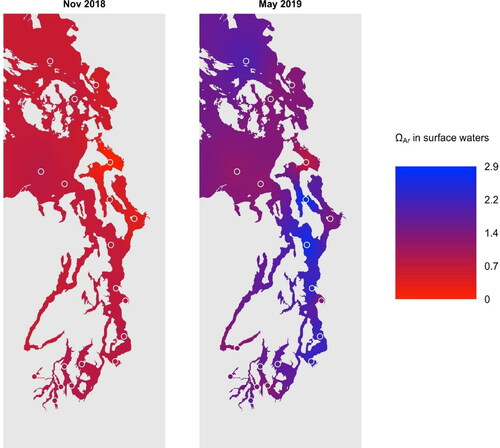
Summary statistics for temperature and salinity and measured (DIC and TA) and calculated marine CO₂ system parameters (pCO₂, pH_T, Ω_Ar and Ω_Ca) from October 2018 to February 2020 at the surface and at 30 m were calculated for each of the seven basins (defined in Table 1) within the study area (Supplementary Materials -Tables S1–S7). DIC and TA at the surface tend to be lower and more variable than at 30 m (Tables S1–S7). On average, surface waters were supersaturated with respect to aragonite between March and September (Ω_Ar > 1), and undersaturated between October and February (Ω_Ar < 1) (Figure 2); data were divided between these two time periods in Tables S1–S7.

Figure 2. Interpolated sea surface aragonite saturation state in greater Puget Sound in November 2018 and May 2019. Open circles indicate stations from which georeferenced data were used.

The range of DIC and TA data collected through Ecology OA monitoring is larger than in datasets collected by other groups in greater Puget Sound (Table 2). This may be due to: (1) the larger geographic range of Ecology OA stations, (2) Ecology OA data are collected year-round, rather than in particular months or seasons (as in Feely et al. (2010) or Roberts, Bos, and Albertson (2008)), (3) reporting full ranges of results rather than ranges of average values (as in Feely et al. (2010)), and (4) inclusion of nearshore stations in Ecology OA monitoring, where influences of freshwater, human activity, and photosynthesis and respiration may drive extreme values. The extant Ecology OA dataset prominently extends the lower ranges of DIC and TA, and these observations coincide with lower salinity waters, commonly in Whidbey Basin. Equally low DIC and TA values have been recorded in Canadian waters of the Salish Sea (Evans et al. 2019; Ianson et al. 2016), where the Fraser River drives low salinities at the surface.

Table 2. Marine CO₂ system data ranges for Ecology OA Monitoring and selected regional studies.

Reference	Region	Time Period	DIC (µmol kg^-1)	TA (µmol kg^-1)	pHT	pCO2 or fCO2 (µatm)	ΩAr
Ecology OA Monitoring	U.S. Salish Sea	Oct 2018 - Feb 2020	558-2182	507-2186	7.18-8.54	85-2764	0.02-3.19
Evans et al. (2019)	Canadian Salish Sea	Dec 2014 - Jun 2018	400-2250	350-2200	7.41-8.59	97.2-869.7	0.44-4.24
Fassbender et al. (2017)	U.S. Salish Sea	2007-2014	Not Reported	1600-2250	Not Reported	Not Reported	Not Reported
Fassbender et al. (2018)*	U.S. Salish Sea	2005-2017	1630-2056	1795-2214	7.67-8.37	161-1311	0.8-3.0
Feely et al. (2010)*	U.S. Salish Sea	Feb/Aug 2008	1881-2264	2018-2268	7.41-8.05	Not Reported	0.40-1.73
Ianson et al. (2016)	Canadian Salish Sea	2003, 2010-2012	1046-2259	1098-2281	Not Reported	Not Reported	Not Reported
Pelletier et al. (2018)	U.S. Salish Sea	Jun 2014 - May 2015	1431-2038	1510-2101	7.51-8.50	100-1417	0.47-3.65
Roberts, Bos, and Albertson (2008)	U.S. Salish Sea	Sep 2006 - Jan 2007	Not Reported	1970-2210	Not Reported	Not Reported	Not Reported

* References only reported ranges of average values of marine CO₂ system data.

Data collected through Ecology OA monitoring corroborate previously observed seasonal patterns. Ω_Ar and Ω_Ca are highest and generally supersaturated (Ω_Ar/Ω_Ca > 1) between March and September (Figure 2) as in Fassbender et al. (2018), Feely et al. (2010), and Pelletier et al. (2018). Chlorophyll data indicate elevated phytoplankton activity from March to September (PSEMP Marine Waters Workgroup (2019)), coincident with increased pH_T and TA and decreased DIC and pCO₂. Spring and summer DIC minima are likely driven by a combination of freshwater delivery (in spring) and consumption of DIC through photosynthesis by phytoplankton (in spring and summer). TA values year-round are tightly coupled with freshwater delivery, as suggested by Fassbender et al. (2018). Chlorohyll decreases in the autumn and winter (PSEMP Marine Waters Workgroup (2019)), when colder temperatures, changes in mixing regimes, and a transition to net heterotrophy cause presumably cause DIC and pCO₂ to increase and pH_T, Ω_Ar, and Ω_Ca to decrease (as in Lowe, Bos, and Ruesink (2019)). Ecology data elucidate the seasonality of OA conditions in greater Puget Sound, especially in shallow, river-dominated areas. These patterns are broadly applicable to coastal and estuarine ecosystems (Carstensen and Duarte 2019).

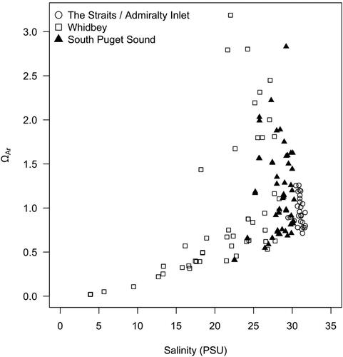
Ecology data also reveal important regional differences in surface water OA conditions (Figure 3). Whidbey Basin exhibited the most variable Ω_Ar values and the lowest Ω_Ar values, which coincided with the lowest observed salinities. By contrast, South Puget Sound Ω_Ar values were moderately variable and salinities remained stable. The Strait of Juan de Fuca and Admiralty Inlet demonstrated low variability in Ω_Ar year-round and high and stable salinities. These differences between basins are large enough that they could have biological consequences. For instance, mean Ω_Ar in Whidbey Basin surface waters from March to September was above the threshold for mild dissolution in pteropods defined by Bednaršek et al. (2020b) (Ω_Ar = 1.5), while mean Ω_Ar in Strait of Juan de Fuca and Admiralty Inlet surface waters over the same period was below that threshold.

Figure 3. Sea surface salinity and aragonite saturation state in selected basins of greater Puget Sound. Data were collected at ADM002 and SJF002 (for the Straits/Admiralty Inlet, which approximates seawater endmember), at SKG003, SAR003, and PSS019 (for Whidbey, where glacial-fed rivers peak in spring), and at BUD005, DNA002, NSQ002, and OAK004 (for South Puget Sound, where rain-fed rivers peak in winter).

Linkages between data & goals of ecology OA monitoring

Ecology OA monitoring was designed to achieve three central goals described in “Introduction.” While the 17 months of data collected between October 2018 and February 2020 is not long enough to realize these goals, Ecology has achieved some initial milestones.

Research goal #1 – Detecting anthropogenic OA through climate-quality data

The primary goal of Ecology OA monitoring is to allow for the eventual detection of long-term decadal anthropogenic effects on OA conditions by collecting ‘climate-quality’ data. GOA-ON defines its weather-level OA data quality objective as ± 10 µmol kg⁻¹ and its climate-quality objective as ± 2 µmol kg⁻¹ for DIC and TA. To assess precision, Ecology collects field duplicate samples for DIC and TA at HCB004 at 30 m, OAK004 at 0 m, SJF002 at 30 m, and GRG002 at 30 m (Table 1 and Figure 1) and calculates mean absolute differences between DIC (mean |ΔDIC|) and TA (mean |ΔTA|) values for field duplicate samples (Table 3). Values of mean |ΔDIC| for field duplicate samples ranged between 0.23 (for GRG002 at 30 m) to 4.01 (for HCB004 at 30 m) µmol kg⁻¹, and values of mean |ΔTA| for field duplicate samples ranged between 1.85 (for GRG002 at 30 m) and 2.72 (for OAK004 at 0 m) µmol kg⁻¹. On a station-by-station basis, these differences exceed weather-level OA data quality objectives and meet or approximate climate-level data quality objectives. The system-wide mean |ΔDIC| and mean |ΔTA| for field duplicate samples are 2.47 µmol kg⁻¹ and 2.35 µmol kg⁻¹, respectively. To assess accuracy, laboratory analyses of Ecology DIC and TA samples are interspersed with analyses of CRMs. To date, the mean absolute difference between measured and certified values is 1.73 µmol kg⁻¹ for DIC and 1.72 µmol kg⁻¹ for TA, exceeding climate-level data quality objectives. Individual absolute differences between measured and certified values of DIC and TA have not exceeded 0.25% of the certified value (Table 4). At the program level, Ecology OA monitoring is therefore meeting the climate-level OA data quality objective in its first 17 months of sample collection across seven basins (Tables S1–S7).

Table 3. Assessment of precision using field duplicate samples collected at QA stations between October 2018 and February 2020.

QA Station (Depth)	Variable (units)	Range	Mean |Δ| between field duplicate samples
HCB004 (30 m)	DIC (µmol kg^-1)	2100-2182	4.01
	TA (µmol kg^-1)	2072-2103	2.45
OAK004 (0 m)	DIC (µmol kg^-1)	1696-1997	1.84
	TA (µmol kg^-1)	1691-2044	2.72
GRG002 (30 m)	DIC (µmol kg^-1)	1912-2078	0.23
	TA (µmol kg^-1)	2053-2104	1.85
SJF002 (30 m)	DIC (µmol kg^-1)	1991-2156	2.96
	TA (µmol kg^-1)	2048-2186	2.06

* GOA-ON weather- and climate-level data quality objectives are ±10 µmol kg^-1 and ±2 µmol kg^-1, respectively, for DIC and TA.

* System-wide mean |ΔDIC| and mean |ΔTA| are ±2.47 and ±2.35 µmol kg^-1, respectively.

Table 4. Assessment of accuracy using CRMs analyzed alongside Ecology OA samples by NOAA PMEL.

Summary Statistic	|Δ| between measured and certified CRM values (µmol kg^-1)		CRM Recovery (%)
	DIC (n = 40)	TA (n = 78)	DIC (n = 40)	TA (n = 78)
Minimum	0.03	0.01	0.00	0.00
25% tile	0.83	0.51	0.04	0.02
Median	1.53	1.21	0.08	0.05
75% tile	2.47	2.48	0.12	0.11
Maximum	4.69	5.30	0.23	0.24
Target	2.00	2.00	<0.25	<0.25

Initial results suggest that Ecology will be able to detect long-term decadal anthropogenic changes in OA conditions as our dataset grows. This is critically important in the context of water quality standards, where determinations of impairment and human influence must rest on robust environmental data.

Research goal #2 – Understanding the role of rivers in regional OA

The second goal of Ecology OA monitoring is to identify and characterize the role of rivers and freshwater in driving regional OA dynamics. Station selection was an important step toward this goal, and river influence was a central criterion in choosing OA monitoring stations (Figure 1). Most of Washington State’s valuable commercial shellfish and bivalve aquaculture activities occur in these shallow, river-forced areas (Blue Ribbon Panel on Ocean Acidification 2012). Between October 2018 and February 2020, 20 of the 518 OA samples collected by Ecology had salinities below 20, compared to only 10 of the 1,203 discrete water samples collected between 2007 and 2014 presented in Fassbender et al. (2017). Through the collection of these low salinity samples, Ecology OA monitoring has illuminated new extremes in OA conditions, including DIC, TA, pH_T, and Ω_Ar (Table 2).

Washington State rivers have lower DIC, TA, and pH relative to seawater in the northeastern Pacific Ocean (Bianucci et al. 2018). In Puget Sound, riverine TA ranges and between 200 and 1300 µmol kg⁻¹, or 10 to 40% of seawater values (Hallock, 2009). Rivers thus effectively dilute TA in estuarine waters, which reduces buffering capacity, decreases pH, and makes these areas more vulnerable to OA. To explore connections between river inputs and OA conditions, we estimated and visualized surface water conditions using the ‘ipdw’ package (0.2-9) in R (4.0.2) to perform inverse path distance weighting to interpolate georeferenced Ecology OA monitoring data across greater Puget Sound following methods developed by Stachelek and Madden (2015). Parts of Whidbey Basin exhibit notably lower Ω_Ar relative to the rest of the region in November 2018 and May 2019 (Figure 2 and Tables S1–S7), likely due to freshwater dilution by Skagit and Snohomish River inputs (Supplementary Materials -Figures S1 and S2). Eighteen of the 20 Ecology OA monitoring samples with salinities below 20 were collected in Whidbey Basin. In Washington State, estuarine areas appear to have reduced buffering capacity (in part due to lower alkalinity), raising the potential of spatially heterogeneous vulnerability to OA. Since climate change is forecasted to drive changes in the hydrological cycle (Bianucci et al. 2018), OA monitoring in estuarine areas is necessary to understand how shifts in the timing and magnitude of river inputs will exacerbate or counteract future acidification.

Research goal #3 – Measuring anthropogenic influences on regional OA conditions

The tertiary goal of Ecology OA monitoring is to determine the effects of regional CO₂ emissions and human nutrient inputs on OA conditions to inform management actions. Station selection was also crucial to advancing this goal. Ecology OA samples are collected in areas far from immediate human influence (e.g., SJF002 and GRG002), and in the shadow of the urban core of the 15^th largest metropolitan area in the USA (ELB015 and PSB003) (Figure 1). These samples provide snapshots of pCO₂, which may reveal correlations or causal relationships with regional CO₂ emissions.

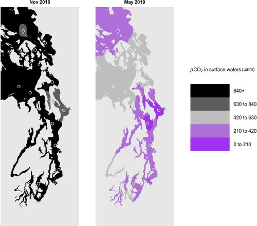
Seawater releases CO₂ into the atmosphere when its pCO₂ value is greater than atmospheric CO₂ concentrations, and seawater absorbs CO₂ when its pCO₂ is below atmospheric levels. Using Ecology OA monitoring data, we estimate that surface waters in greater Puget Sound were releasing CO₂ into the atmosphere throughout the region in November 2018 (Figure 4) – a condition that persisted for most of the fall and winter. In contrast, we estimate that large swaths of surface waters were absorbing CO₂ from the regional atmosphere in May 2019 (Figure 4). These estimates suggest that any sensitivity to regional CO₂ emissions is seasonal and spatially variable. In the future, Ecology OA monitoring data will be integrated with data on regional sources of CO₂ emissions, local atmospheric CO₂ concentrations, and on eutrophication and local nutrient inputs to explore anthropogenic influences on OA conditions.

Figure 4. Interpolated sea surface pCO₂ in greater Puget Sound in November 2018 and May 2019. Open circles indicate stations from which georeferenced data were used. A pCO₂ value of 420 μatm represents the nominal regional atmospheric CO₂ concentration, and therefore, the transition between waters undersaturated and oversaturated with respect to atmospheric CO₂ that serve as CO₂ sinks (dark and light purple) from and CO₂ sources (greys and black) to the atmosphere, respectively.

Challenges & lessons learned

Over the course of designing and implementing a large-scale OA monitoring program in a dynamic nearshore estuarine system, we overcame challenges that are likely to confront scientists and natural resource managers in other jurisdictions undertaking similar OA monitoring work. These include:

1. Addition of mercuric chloride - Community-standard OA Best Practices dictate that DIC and TA samples should be preserved with mercuric chloride immediately after collection in the field (Dickson, Sabine, and Christian 2007). We found that this is not always practicable: vessel size, available space, and stability in transit may prohibit immediate addition of mercuric chloride due to safety concerns. Some jurisdictions may even prohibit the use of mercury altogether. We overcame our challenge by implementing immediate sample filtration in the field, and delaying the addition of mercuric chloride until controlled conditions are gained upon return to the laboratory (as in Keyzers 2016; Leinweber and Gruber 2013; Pelletier et al. 2018). Despite this departure from best practices, Ecology DIC and TA data fall within ranges observed by other groups in the region (Table 2) and meet GOA-ON climate-level data quality standards (Table 3).

2. Field duplicates for quality control – Ecology OA field duplicate samples are used to evaluate field replication and precision. Initially, field duplicate samples were collected at stations selected for convenience. We discovered that field duplicates collected in surface waters near rivers exhibited notable differences in DIC and/or TA. Under these circumstances, field duplicates were likely drawn from Niskin bottles that captured water from different water masses with different properties. We selected a new set of stations for field duplicates, with most of our samples collected at 30m, where we expected conditions to be less dynamic.

3. Accurate salinity data – Ecology OA monitoring measures DIC and TA, but secondary environmental data such as salinity are just as important. The effects of inaccurate or imprecise salinity data will propagate through marine CO₂ system calculations and lead to inaccuracies and inconsistencies in calculated marine CO₂ system parameters (e.g., Ω_Ar and pH_T). We therefore collect discrete water samples for salinity alongside samples for DIC and TA, and use CTD salinity data only when discrete water samples for salinity are unavailable. We believe this has improved the accuracy of our calculated CO₂ system parameters, but the collection of additional discrete water samples has imposed additional costs on our monitoring program. We recommend that other OA monitoring programs give careful consideration to the accuracy of secondary environmental data.

4. Partnering with an analytical laboratory – Jurisdictions seeking to implement OA monitoring are unlikely to have the established capacity to measure marine CO₂ system parameters such as DIC and TA. Rather than developing that capacity from the ground up, we recommend forming a partnership with an analytical laboratory. The exceptional quality of Ecology OA monitoring data would not be possible without our collaboration with NOAA PMEL. Ecology, however, is fortunate since Washington State has been a hub for OA research for the last 25 years and regional research partners like NOAA PMEL are located here. If careful attention is paid to sample chain-of-custody and tracking, then shipping samples may also be practical for monitoring programs without geographic proximity to a partner laboratory. We also recommend maintaining clear and open lines of communication, clarifying the timing and frequency of sample deliveries and supply procurement, and developing a common understanding around data delivery and sharing.

5. Station selection – Jurisdictions developing OA monitoring programs should consult existing data (if any) on local and regional marine CO₂ chemistry, identify data gaps, and articulate goals before selecting stations. Logistical constraints such as budgets, geographic convenience, station bottom depth and tidal range, number of available Niskin bottles, and water budgets (i.e., volume of Niskin bottles) will also guide what is possible. Although consistency is important in any monitoring program, we recommend maintaining some amount of flexibility in the early years of OA monitoring. In our case, some stations have proved to be redundant, with nearly identical DIC and TA values measured at geographically proximate station pairs. While redundancy is useful for some applications, it can also impose unnecessary costs on a monitoring program. We have adjusted our station selections to drop redundant stations and substitute stations in areas where OA conditions are less understood.

Considerations for program design

OA monitoring programs undertaken elsewhere could benefit from additional activities, including:

1. Expand DIC and TA sampling into rivers – In estuarine systems, rivers can drive circulation, deliver nutrients, and reduce buffering capacity through the dilution of TA (Bianucci et al. 2018; Fassbender et al. 2018; Pelletier et al. 2018). Climate change will alter hydrological cycles, including the magnitude and seasonality of river inputs (Bianucci et al. 2018). To quantify current hydrological variability and better understand how future shifts in hydrological cycles will impact OA conditions, it may be valuable to expand the monitoring of DIC, TA, or other marine CO₂ system parameters into rivers to gather baseline data and to detect long-term changes.

2. Add Monitoring for Calcium Ion Concentrations ([Ca^2±]) – Ocean acidification and the subsequent decreases in pH drive decreases in $\left[{\mathrm{CO}}_3^{2-}\right]$ and CaCO₃ mineral saturation states (Ω) in aquatic systems. Recent work has shown the uncertainty in [Ca²⁺] cause GOA-ON climate data quality objectives for Ω (or calculating Ω with a relative uncertainty of ≤1%; Newton et al. 2015) to be surpassed in dynamic and variable nearshore coastal and estuarine waters (Dillon et al. 2020). This occurs due to relatively minor local deviations (<4%) from global conservative [Ca²⁺]-salinity relationships (e.g., Riley and Tongudai (1967)) that are used to estimate [Ca²⁺] from salinity when calculating Ω in programs like SeaCarb (Gattuso et al. 2020). Further, GOA-ON weather-level data quality objectives for Ω (±0.2 in computational accuracy) (McLaughlin et al. 2015; Newton et al. 2015) could also be surpassed depending on the magnitude of local deviations from [Ca²⁺]-salinity relationships; which additional analyses of jurisdiction-specific OA and water quality data can help elucidate (Dillon et al. 2020) This ultimately results in inaccurate and/or imprecise estimates of Ω_Ar and Ω_Ca (Dillon et al. 2020). Coincidentally, this may warrant adding monitoring for [Ca²⁺] to long-term OA monitoring programs; especially if the creation of water quality standards based on Ω_Ar and/or Ω_Ca using its data is one of its underlying goals.

3. Conduct analysis of marine CO₂system parameters in-house – Many regulatory agencies have associated analytical laboratories – for example, Manchester Environmental Laboratory (Port Orchard, WA, USA) conducts other analyses for Ecology. If such laboratories are interested in exploring the addition of analytical capacity to measure DIC, TA, and/or pH, careful consideration must be given to the methods and instruments used and all should conform with OA community-standard methods (as in Dickson, Sabine, and Christian 2007). Before the analysis of field samples begins, laboratories should acquire and perform replicate analyses of CRMs used in inter-laboratory comparison experiments (Bockmon and Dickson 2015) to determine the accuracy and precision of adopted methods. Such steps are needed to ensure consistency and comparability across OA datasets. Finally, laboratories need to reconcile the cost and time it will take to develop methods, purchase instruments, hire and train staff, and perform other steps needed to accomplish this goal with the overarching plan and timeline for their OA monitoring work (as this could possibly delay the start of sampling by multiple years).

Conclusions

Ecology designed and implemented a large-scale OA monitoring program, focused on the nearshore river-influenced areas of greater Puget Sound. Ecology OA monitoring aims to produce high quality DIC and TA data to detect long-term decadal anthropogenic effects on regional OA conditions amidst natural variability, to uncover the role of rivers on OA dynamics, and to explore the impacts of regional CO₂ emissions and nutrient inputs on OA conditions to inform management actions. Over the first 17 months of OA monitoring, between October 2018 and February 2020, Ecology has produced a dataset that meets GOA-ON climate-level data quality objectives for DIC and TA, extends the lower ranges of observed marine CO₂ system data in the region, and demonstrates the strong effects of river inputs on OA conditions in parts of greater Puget Sound. Ecology OA monitoring has also corroborated patterns in OA conditions observed by other groups. To aid in the development of OA monitoring programs elsewhere, we recounted lessons learned and offered considerations for program design that could enhance the utility of OA monitoring in other contexts.

Acidification in the open ocean can only be controlled by reducing global CO₂ emissions, but acidification in nearshore systems might be mitigated through tangible actions like reducing regional CO₂ emissions, reducing local nutrient inputs, or through alkalinity additions or phytoremediation (Carstensen and Duarte 2019; Rheuban et al. 2019; Weisberg et al. 2016). Local and regional jurisdictions that might take these tangible actions need OA monitoring programs that are tailored to generate data in support of regulatory decision-making. In the United States, Washington was early to recognize and respond to the threat of OA, and a broad partnership between the shellfish industry, academic institutions, federal agencies, and state agencies has advanced OA science on many fronts. Ecology’s OA monitoring program can serve as a blueprint alongside the existing literature to design nearshore monitoring programs undertaken by subnational jurisdictions as part of a coordinated effort for OA response – a strategy that has been effective in Washington State.

Acknowledgements

We sincerely thank staff of NOAA’s Pacific Marine Environmental Laboratory for their assistance with the low salinity TA method development work and laboratory analyses of DIC and TA samples. We thank staff of University of Washington’s Marine Chemistry Laboratory for their assistance with laboratory analyses of nutrient and salinity samples. We thank staff of the Shannon Point Marine Center and Western Washington University for their help with conducting monitoring work in Whidbey Basin and stations outside of the Sound proper. We thank Sandy Weakland for help with map generation in ArcGIS. We thank Ecology’s Quality Assurance Officers and Publications Team for supporting the timely preparation, review, and publication of project materials. Finally, we thank Danielle Dixson of University of Delaware for delivering the writing course that guided the preparation of this paper. Financial support for this work was and continues to be provided by a grant from the Puget Sound National Estuary Program, NTA 2016-0408 (‘Add Ocean Acidification Parameters to Ecology’s Monitoring’). In 2019, the Washington State Legislature approved an allocation from the State’s General Fund to support this work.

References

- Aufdenkampe, A. K., E. Mayorga, P. A. Raymond, J. M. Melack, S. C. Doney, S. R. Alin, R. E. Aalto, and K. Yoo. 2011. Riverine coupling of biogeochemical cycles between land, oceans, and atmosphere. Frontiers in Ecology and the Environment 9 (1):53–60. doi: https://doi.org/10.1890/100014.
- Badocco, D., F. Pedrini, A. Pastore, V. di Marco, M. G. Marin, S. Bogialli, et al. 2020. Use of a simple empirical model for the accurate conversion of the seawater pH value measured with NIST calibration into seawater pH scales. Talanta 225: 122051.
- Banas, N. S., L. Conway-Cranos, D. A. Sutherland, P. MacCready, P. Kiffney, and M. Plummer. 2015. Patterns of river influence and connectivity among subbasins of Puget Sound, with application to bacterial and nutrient loading. Estuaries and Coasts 38 (3):735–53. doi: https://doi.org/10.1007/s12237-014-9853-y.
- Bates, N., Y. Astor, M. Church, K. Currie, J. Dore, M. Gonaález-Dávila, L. Lorenzoni, F. Muller-Karger, J. Olafsson, and M. Santa-Casiano. 2014. A time-series view of changing surface ocean chemistry due to ocean uptake of anthropogenic CO2 and ocean acidification. Oceanography 27 (1):126–41. doi: https://doi.org/10.5670/oceanog.2014.16.
- Bednaršek, N., R. A. Feely, M. W. Beck, S. R. Alin, S. A. Siedlecki, P. Calosi, E. L. Norton, C. Saenger, J. Štrus, D. Greeley, et al. 2020a. Exoskeleton dissolution with mechanoreceptor damage in larval Dungeness crab related to severity of present-day ocean acidification vertical gradients. Science of the Total Environment 716:136610. doi: https://doi.org/10.1016/j.scitotenv.2020.136610.
- Bednaršek, N., G. Pelletier, A. Ahmed, and R. A. Feely. 2020b. Chemical Exposure Due to Anthropogenic Ocean Acidification Increases Risks for Estuarine Calcifiers in the Salish Sea: Biogeochemical Model Scenarios. Frontiers in Marine Science 7:580. doi: https://doi.org/10.3389/fmars.2020.00580.
- Bianucci, L., W. Long, T. Khangaonkar, G. Pelletier, A. Ahmed, and T. Mohamedali. 2018. Sensitivity of the regional ocean acidification and carbonate system in Puget Sound to ocean and freshwater inputs. Elementa: Science of the Anthropocene 6 (1):22. doi: https://doi.org/10.1525/elementa.151/112790
- Blue Ribbon Panel on Ocean Acidification. 2012. Ocean acidification: From knowledge to action, Washington State’s Strategic Response. Publication No. 12-01-015. Washington State Department of Ecology, Olympia. https://fortress.wa.gov/ecy/publications/SummaryPages/1201015.html
- Bockmon, E. E., and A. G. Dickson. 2015. An inter-laboratory comparison assessing the quality of seawater carbon dioxide measurements. Marine Chemistry 171:36–43. doi: https://doi.org/10.1016/j.marchem.2015.02.002.
- Bos, J., M. Keyzers, L. Hermanson, C. Krembs, and S. Albertson. 2015. Quality assurance monitoring plan: Long-term marine waters monitoring, Water Column Program. Publication No. 15-03-101. Washington State Department of Ecology, Olympia. https://fortress.wa.gov/ecy/publications/SummaryPages/1503101.html
- Burns, R. E. 1985. The shape and form of Puget Sound. Seattle, WA, USA: Washington Sea Grant. 100. pp.
- Bushinsky, S. M., Y. Takeshita, and N. L. Williams. 2019. Observing changes in ocean carbonate chemistry: Our autonomous future. Current Climate Change Reports 5 (3):207–20. doi: https://doi.org/10.1007/s40641-019-00129-8.
- Butler, R. A., A. K. Covington, and M. Whitfield. 1985. The determination of pH in estuarine waters. II: Practical considerations. Oceanologica Acta 8 (4):433–9.
- Cai, W.-J., R. A. Feely, J. M. Testa, M. Li, W. Evans, S. R. Alin, et al. 2020. Natural and Anthropogenic Drivers of Acidification in Large Estuaries. Annual Review of Marine Science 13:23-55.
- Caldeira, K., and M. E. Wickett. 2003. Oceanography: anthropogenic carbon and ocean pH. Nature 425 (6956):365.
- Carstensen, J., and C. M. Duarte. 2019. Drivers of pH variability in coastal ecosystems. Environmental Science & Technology 53 (8):4020–4029. doi: https://doi.org/10.1021/acs.est.8b03655.
- Chai, F., K. S. Johnson, H. Claustre, X. Xing, Y. Wang, E. Boss, et al. 2020. Monitoring ocean biogeochemistry with autonomous platforms. Nature Reviews Earth & Environment, 1 (6):315–26. https://www.nature.com/articles/s43017-020-0053-y
- Dickson, A. G., C. L. Sabine, and J. R. Christian. 2007. Guide to best practices for ocean CO2 measurements. Sidney, BC, Canada: North Pacific Marine Science Organization. https://meetings.pices.int/contact/main
- Dillon, W. D., P. W. Dillingham, K. I. Currie, and C. M. McGraw. 2020. Inclusion of uncertainty in the calcium-salinity relationship improves estimates of ocean acidification monitoring data quality. Marine Chemistry 226:103872. doi: https://doi.org/10.1016/j.marchem.2020.103872.
- Duarte, C. M., I. E. Hendriks, T. S. Moore, Y. S. Olsen, A. Steckbauer, L. Ramajo, J. Carstensen, J. A. Trotter, and M. McCulloch. 2013. Is ocean acidifcation an open-ocean syndrome? Understanding anthropogenic impacts on seawater pH. Estuaries and Coasts 36 (2):221–236. doi: https://doi.org/10.1007/s12237-013-9594-3.
- Easley, R. A., and R. H. Byrne. 2012. Spectrophotometric calibration of pH electrodes in seawater using purified m-cresol purple. Environmental Science & Technology 46 (9):5018–5024. doi: https://doi.org/10.1021/es300491s.
- Evans, W., K. Pocock, A. Hare, C. Weekes, B. Hales, J. Jackson, H. Gurney-Smith, J. T. Mathis, S. R. Alin, R. A. Feely, et al. 2019. Marine CO2 patterns in the northern Salish Sea. Frontiers in Marine Science 5:536. doi: https://doi.org/10.3389/fmars.2018.00536.
- Fassbender, A. J., S. R. Alin, R. A. Feely, A. J. Sutton, J. A. Newton, and R. H. Byrne. 2017. Estimating total alkalinity in the Washington State coastal zone: Complexities and surprising utility for ocean acidification research. Estuaries and Coasts 40 (2):404–418. doi: https://doi.org/10.1007/s12237-016-0168-z.
- Fassbender, A. J., S. R. Alin, R. A. Feely, A. J. Sutton, J. A. Newton, C. Krembs, J. Bos, M. Keyzers, A. Devol, W. Ruef, et al. 2018. Seasonal carbonate chemistry variability in marine surface waters of the US Pacific Northwest. Earth System Science Data 10 (3):1367–1401. doi: https://doi.org/10.5194/essd-10-1367-2018.
- Feely, R. A., S. R. Alin, J. Newton, C. L. Sabine, M. Warner, A. Devol, C. Krembs, and C. Maloy. 2010. The combined effects of ocean acidification, mixing, and respiration on pH and carbonate saturation in an urbanized estuary. Estuarine, Coastal and Shelf Science 88 (4):442–449. doi: https://doi.org/10.1016/j.ecss.2010.05.004.
- Feely, R. A., C. L. Sabine, J. M. Hernandez-Ayon, D. Ianson, and B. Hales. 2008. Evidence for upwelling of corrosive "acidified" water onto the continental shelf. Science 320 (5882):1490–1492. doi: https://doi.org/10.1126/science.1155676.
- Freelan, S. 2009. Map of the Salish Sea (Mer des Salish) & Surrounding Basin. Western Washington University, Bellingham. http://staff.wwu.edu/stefan/salish_sea.shtml.
- Gattuso, J.-P., J.-P. Epitalon, H. Lavigne, and J. Orr. 2020. Seacarb Seawater Carbonate Chemistry. Package 3.2.13. https://cran.r-project.org/web/packages/seacarb/index.html.
- Gattuso, J.-P., A. Magnan, R. Billé, W. W. L. Cheung, E. L. Howes, F. Joos, D. Allemand, L. Bopp, S. R. Cooley, C. M. Eakin, et al. 2015. OCEANOGRAPHY. Contrasting futures for ocean and society from different anthropogenic CO₂ emissions scenarios. Science 349 (6243):aac4722. doi: https://doi.org/10.1126/science.aac4722.
- Gonski, S. F., W.-J. Cai, W. J. Ullman, A. Joesoef, C. R. Main, D. T. Pettay, and T. R. Martz. 2018. Assessment of the suitability of Durafet-based sensors for pH measurement in dynamic estuarine environments. Estuarine, Coastal and Shelf Science 200:152–168. doi: https://doi.org/10.1016/j.ecss.2017.10.020.
- Gonski, S., C. Krembs, and G. Pelletier. 2019. Quality assurance project plan: Ocean acidification monitoring at ecology’s greater puget sound stations. Publication No. 19-03-102. Washington State Department of Ecology, Olympia. https://fortress.wa.gov/ecy/publications/SummaryPages/1903102.html.
- Harris, K. E., M. D. DeGrandpre, and B. Hales. 2013. Aragonite saturation state dynamics in a coastal upwelling zone. Geophysical Research Letters 40 (11):2720–2725. doi: https://doi.org/10.1002/grl.50460.
- Herrera Environmental Consultants, Inc. 2011. Toxics in surface runoff to puget sound: Phase 3 data and load estimates. Publication No. 11-03-010. Washington State Department of Ecology, Olympia. https://fortress.wa.gov/ecy/publications/publications/1103010.pdf.
- Ianson, D., S. E. Allen, B. L. Moore-Maley, S. C. Johannessen, and A. R. W. Macdonald. 2016. Vulnerability of a semienclosed estuarine sea to ocean acidification in contrast with hypoxia. Geophysical Research Letters 43 (11):5793–5801. doi: https://doi.org/10.1002/2016GL068996.
- IPCC. 2013. Summary for policymakers. In Climate change 2013: The physical science basis. Contribution of Working Group I to the Fifth Assessment Report of the Intergovernmental Panel on Climate Change, ed. T. F. Stocker, D. Qin, G. K. Plattner, M. Tignor, S. K. Allen, et al. Cambridge, UK; Newyork, NY, USA: Cambridge University Press.
- Kennish, J. 1998. Pollution impacts on marine biotic communities. Boca Raton, FL, USA: CRC Press, 336pp.
- Keyzers, M. 2014. Quality assurance project plan: Puget Sound total alkalinity and dissolved inorganic carbon pilot project. Publication No. 14-03-116. Washington State Department of Ecology, Olympia. https://fortress.wa.gov/ecy/publications/SummaryPages/1403116.html.
- Keyzers, M. 2016. Puget Sound Total Alkalinity and Dissolved Inorganic Carbon Pilot Project. Publication No. 16-03-032. Washington State Department of Ecology, Olympia. https://fortress.wa.gov/ecy/publications/SummaryPages/1603032.html.
- Keyzers, M., A. Brownlee, and C. Krembs. 2019. Addendum 6 to Quality Assurance Monitoring Program: Long-Term Marine Waters Monitoring. Water Column Program. Publication No. 19. 03-107. Washington State Department of Ecology, Olympia. https://fortress.wa.gov/ecy/publications/SummaryPages/1903107.html.
- Leinweber, A., and N. Gruber. 2013. Variability and trends of ocean acidification in the Southern California Current System: A time series from Santa Monica Bay. Journal of Geophysical Research: Oceans 118 (7):3622–3633.
- Lowe, A. T., J. Bos, and J. Ruesink. 2019. Ecosystem metabolism drives pH variability and modulates long-term ocean acidification in the Northeast Pacific coastal ocean. Scientific Reports 9 (1):1–11. doi: https://doi.org/10.1038/s41598-018-37764-4.
- Martell-Bonet, L., and R. H. Byrne. 2020. Characterization of the nonlinear salinity dependence of glass pH electrodes: A simplified spectrophotometric calibration procedure for potentiometric seawater pH measurements at 25° C in marine and brackish waters: 0.5≤ S≤ 36. Marine Chemistry 220:103764. doi: https://doi.org/10.1016/j.marchem.2020.103764.
- McLaughlin, K., S. Weisberg, A. Dickson, G. Hofmann, J. Newton, D. Aseltine-Neilson, A. Barton, S. Cudd, R. Feely, I. Jefferds, et al. 2015. Core principles of the California Current Acidification Network: Linking chemistry, physics, and ecological effects. Oceanography 25 (2):160–169. doi: https://doi.org/10.5670/oceanog.2015.39.
- Millero, F. J. 1986. The pH of estuarine waters. Limnology and Oceanography 31 (4):839–847. doi: https://doi.org/10.4319/lo.1986.31.4.0839.
- Mohamedali, T., M. Roberts, B. Sackmann, and A. Kolosseus. 2011. Puget Sound dissolved oxygen model nutrient and load summary for 1999-2008. Publication No. 11-03-057. Washington State Department of Ecology, Olympia. https://fortress.wa.gov/ecy/publications/SummaryPages/1103057.html
- Moore-Maley, B. L., S. E. Allen, and D. Ianson. 2016. Locally driven interannual variability of near‐surface pH and ΩA in the Strait of Georgia. Journal of Geophysical Research: Oceans 121 (3):1600–1625.
- Newton, J. A., R. A. Feely, E. B. Jewett, P. Williamson, and J. Mathis. 2015. Global ocean acidification observing network: Requirements and governance plan.
- Pelletier, G., M. Roberts, M. Keyzers, and S. R. Alin. 2018. Seasonal variation in aragonite saturation in surface waters of Puget Sound—A pilot study. Elementa: Science of the Anthropocene 6 (1):5.
- Pettay, D. T., S. F. Gonski, W.-J. Cai, C. K. Sommerfield, and W. J. Ullman. 2020. The ebb and flow of protons: A novel approach for the assessment of estuarine and coastal acidification. Estuarine, Coastal and Shelf Science 236:106627. doi: https://doi.org/10.1016/j.ecss.2020.106627.
- Pimenta, A. R., and J. S. Grear. 2018. Guidelines for measuring changes in seawater pH and associated carbonate chemistry in coastal environments of the Eastern United States.
- Provoost, P., S. Van Heuven, K. Soetaert, R. W. P. M. Laane, and J. J. Middelburg. 2010. Seasonal and long-term changes in pH in the Dutch coastal zone. Biogeosciences 7 (11):3869–3878. doi: https://doi.org/10.5194/bg-7-3869-2010.
- PSEMP Marine Waters Workgroup. 2019. Puget Sound marine waters: 2019 overview (J. Apple, R. Wold, K. Stark, J. Bos, P. Williams, N. Hamel, S. Yang, J. Selleck, S. Moore, J. Rice, S. Kantor, C. Krembs, G. Hannach, and J. Newton (eds.)). Olympia, WA: The Puget Sound Partnership.
- Rheuban, J. E., S. C. Doney, D. C. McCorkle, and R. W. Jakuba. 2019. Quantifying the effects of nutrient enrichment and freshwater mixing on coastal ocean acidification. Journal of Geophysical Research: Oceans 124 (12):9085–9100. doi: https://doi.org/10.1029/2019JC015556.
- Riley, J. P., and M. Tongudai. 1967. The major cation/chlorinity ratios in sea water. Chemical Geology 2:263–269. doi: https://doi.org/10.1016/0009-2541(67)90026-5.
- Roberts, M., J. Bos, and S. Albertson. 2008. South puget sound dissolved oxygen study interim data report. Publication No. 08-03-037. Washington State Department of Ecology, Olympia. https://fortress.wa.gov/ecy/publications/SummaryPages/0803037.html.
- Sabine, C. L., H. Ducklow, and M. Hood. 2010. International carbon coordination: Roger Revelle’s legacy in the. Oceanography 23 (3):48–61. doi: https://doi.org/10.5670/oceanog.2010.23.
- Sabine, C. L., R. A. Feely, N. Gruber, R. M. Key, K. Lee, J. L. Bullister, R. Wanninkhof, C. S. Wong, D. W. R. Wallace, B. Tilbrook, et al. 2004. The oceanic sink for anthropogenic CO2. Science 305 (5682):367–371. doi: https://doi.org/10.1126/science.1097403.
- Sastri, A. R., J. R. Christian, E. P. Achterberg, D. Atamanchuk, J. J. H. Buck, P. Bresnahan, P. J. Duke, W. Evans, S. F. Gonski, B. Johnson, et al. 2019. Perspectives on in situ sensors for ocean acidification research. Frontiers in Marine Science 6:653. doi: https://doi.org/10.3389/fmars.2019.00653.
- Stachelek, J., and C. J. Madden. 2015. Application of inverse path distance weighting for high-density spatial mapping of coastal water quality patterns. International Journal of Geographical Information Science 29 (7):1240–1250. doi: https://doi.org/10.1080/13658816.2015.1018833.
- Su, J., W.-J. Cai, J. Brodeur, B. Chen, N. Hussain, Y. Yao, C. Ni, J. M. Testa, M. Li, X. Xie, et al. 2020. Chesapeake Bay acidification buffered by spatially decoupled carbonate mineral cycling. Nature Geoscience 13 (6):441–7. doi: https://doi.org/10.1038/s41561-020-0584-3.
- Tilbrook, B., E. B. Jewett, M. D. DeGrandpre, J. M. Hernandez-Ayon, R. A. Feely, D. K. Gledhill, L. Hansson, K. Isensee, M. L. Kurz, J. A. Newton, et al. 2019. An enhanced ocean acidification observing network: From people to technology to data synthesis and information exchange. Frontiers in Marine Science 6:337. doi: https://doi.org/10.3389/fmars.2019.00337.
- Waldbusser, G. G., B. Hales, C. J. Langdon, B. A. Haley, P. Schrader, E. L. Brunner, M. W. Gray, C. A. Miller, and I. Gimenez. 2015. Saturation-state sensitivity of marine bivalve larvae to ocean acidification. Nature Climate Change 5 (3):273–280. doi: https://doi.org/10.1038/nclimate2479.
- Wallace, R. B., H. Baumann, J. S. Grear, R. C. Aller, and C. J. Gobler. 2014. Coastal ocean acidification: The other eutrophication problem. Estuarine, Coastal and Shelf Science 148:1–13. doi: https://doi.org/10.1016/j.ecss.2014.05.027.
- Washington Administrative Code. 2019 WAC 173-201A-210. Marine water designated uses and criteria.
- Weisberg, S. B., N. Bednaršek, R. A. Feely, F. Chan, A. B. Boehm, M. Sutula, J. L. Ruesink, B. Hales, J. L. Largier, J. A. Newton, et al. 2016. Water quality criteria for an acidifying ocean: Challenges and opportunities for improvement. Ocean & Coastal Management 126:31–41. doi: https://doi.org/10.1016/j.ocecoaman.2016.03.010.
- Wittmann, A. C., and H. O. Pörtner. 2013. Sensitivities of extant animal taxa to ocean acidification. Nature Climate Change 3 (11):995–1001. doi: https://doi.org/10.1038/nclimate1982.