Computing properties of the hydrogen dissociation reaction in and away from equilibrium

Abstract

We study the dissociation of hydrogen from molecule to atoms and show how we can compute thermodynamic and transport properties of both species in a mixture under non-ideal conditions. The small system method can be used to sample fluctuations of a few atoms or molecules in a small volume element, and gives fast access to accurate thermodynamic data of mixtures that are non-ideal. From the results of equilibrium and non-equilibrium molecular dynamics simulations of the dissociation of hydrogen in a thermal field, we compute coefficients for transport of heat and mass for the gas mixture (0.0052 g cm) at average temperature 10400 K. We show that the interdiffusion coefficient, the thermal conductivity and the Dufour effect are significantly affected by the presence of the reaction.

Keywords:

• Small system method
• enthalpy of reaction
• thermodynamic factor
• chemical potential

1. Introduction

The aim of this work is to describe a new procedure to find thermodynamic properties of a chemical reaction and use these properties to study a chemical reaction that is exposed to a thermal field, i.e. a gradient in temperature. The presence of a chemical reaction changes the way energy is stored in a system, e.g. through the formation or breaking of bonds. This also affects transport of heat and mass, as we shall see in a chemical reactor, reactions will often take place under severe temperature gradients.[1] Away from chemical and thermal equilibrium, components diffuse and react; and at the same time, the particles serve as transporters of heat. As an example, we take the hydrogen dissociation reaction:(1)

which takes place on the sun at  K.[2–4] In the chemical industry, this reaction is relevant for separation of hydrogen gas from a gas mixture (e.g. hydrogen gas from CO, water, and CO in the water-gas shift reaction).[5,6] The fact that the reaction itself may contribute to heat transfer was investigated already in 1912 by Langmuir [7]. When the temperature approached 3500 K, he found a large increase in the thermal conductivity and explained it by dissociation of hydrogen. From the data, he estimated an enthalpy of reaction at constant pressure near 550 KJ mol, while today the value is estimated to be 435 KJ mol [8–10] under standard temperature and pressure. The purpose of this article is to find accurate thermodynamic data as well as transport coefficients for the hydrogen dissociation reaction. We present a recent theoretical formulation of the non-equilibrium problem. Molecular dynamics simulations are used to find the relevant data. The simulated systems are at high temperatures and pressures, conditions that can be difficult to manage in a laboratory.

Equilibrium data are necessary in order to compute the driving forces of the system. Therefore, we first describe the system at equilibrium (Section 2), highlighting results obtained earlier by Skorpa et al. [11,12]. The flux equations are then derived from the entropy production and the resulting transport coefficients are determined.[13] We shall see that the interdiffusion coefficient defined for this particular system is far from the diffusion coefficients that can be computed for single gas components by kinetic theory gases.

It is cumbersome to obtain reliable thermodynamic data for non-ideal mixtures in experiments as well as by computer simulations, e.g. see Hafskjold and Ikeshoji [14]. In particular, it is difficult to find partial molar enthalpies, reaction enthalpies and activity coefficients. With the advent of the small system method,[15–17], we can find such properties in a single simulation by sampling particle fluctuations in small volume elements. We repeat an explanation of this method in Sections 3 and 5, and give the results used to compute of transport properties for the hydrogen mixture.

To the best of our knowledge, there is no other systematic molecular dynamics simulation study of transport properties in a chemically reactive mixture. We base this study on the theoretical description first presented by de Groot and Mazur [18]. This was extended on by Xu et al. [19–21], who did simulations on the fluoride dissociation reaction. Most of the simulations and methods presented in this article have been discussed in more detail in recent works [11–13,22] for a liquid-like mixture, a dense gas and a dilute gas. The present work is an in-depth analysis of the gas mixture alone, giving an overview of results for this system. The aim is to set in perspective several new methods of analysis, so that they can be useful for other systems. In this manner, we hope to contribute to the creation of transport data that are needed in the context of chemical reaction engineering and research on reacting mixtures.

2. The hydrogen dissociation reaction

2.1. Particle interaction potentials

A full description and analysis of the interaction potential for hydrogen atom and molecule was presented already by Skorpa et al. [11]. The most essential parts are repeated here in order to be able to discuss the properties of the model. The hydrogen dissociation reaction can be modelled accurately with classical interaction potentials derived from quantum mechanics.[10,19,20,23] Stillinger and Weber [23] showed that it was sufficient to use a classical interaction potential, U, which is the sum of two- and three-particle interaction contributions, in order to describe the essentials of a chemical reaction:(2)

where and are the two- and three-particle potentials, respectively (see in Equations (3(3) ) and (4(4) )). Diedrich and Anderson [24,25] and Kohen et al. [10] derived expressions for two- and three-particle potentials of hydrogen. The functional form of the two-particle contribution term is:(3)

where , , , and are hydrogen-specific parameters.[10] The value was chosen such that the minimum of the potential gives the bond dissociation energy of hydrogen (432.065 kJ mol [10]) at the bond distance between two hydrogen atoms, .[24] When the distance between two atoms is larger than the cut-off distance, , the potential is zero.

The functional form of the three-particle contribution is the sum of the individual contributions from each particle:(4)

where the h-functions in this expressions are given by:(5)

and(6)

Here, , , and are constants.[10] The cut-off distance, , is the same for both the two- and three-particle interactions (2.8 Å). The interaction potential that we use has a short range, and no long-range correction was used. The is the angle between and . In the triad subscript j, i, k, the middle letter i refers to the atom at the subtended angle vertex. The role of the three-particle interaction term is to prevent formation of more than one bond between hydrogen atoms.

The transition from atomic to molecular hydrogen was based on the bond length between the interaction centres of the hydrogen atoms. When the distance between two particles was shorter than in reduced units, they were labelled as part of a molecule. This is in agreement with the procedure used by Stillinger and Weber [23]. More on the use of reduced variables can be found in Table 1. All reduced variables are denoted by an asterisk.

3. The chemical reaction in equilibrium

3.1. Thermodynamic relations

The enthalpy change of the hydrogen dissociation reaction is given by the partial molar enthalpies of the components(7)

where , and i is either hydrogen atom or molecule. The reaction Gibbs energy is likewise:(8)

The chemical potential of a component is defined relative to the chemical potential of an ideal gas of 1 bar pressure (the standard chemical potential ):(9)

The fugacity of the gas component, , is equal to the partial pressure of the gas, , times the fugacity coefficient . Superscript denotes the standard state (1 bar). We introduce Equation (9(9) ) into Equation (8(8) ) and use the condition for chemical equilibrium, . This gives the thermodynamic equilibrium constant :(10)

where . The equilibrium constant can also be expressed in terms of the dissociation constant, , or the pressure-based dissociation constant: . Here, P is the total pressure. The activity coefficient ratio is defined via:(11)

The equilibrium constant can be found from the van’t Hoff equation at constant pressure. If the enthalpy of reaction is known at standard conditions, then:(12)

In the presence of a varying pressure, there is an additional term in this equation:(13)

where the last term gives the pressure dependence, with as the reaction volume.

3.2. Fluctuations and scaling laws

The thermodynamic correction factor, , is defined as:(14)

where , is the Boltzmann’s constant, is the chemical potential and subscripts i and j denote the two components. At constant (), we determine from the fluctuation theory formula derived by Reed and Ehrlich [26]:(15)

The small system method gives the inverse of the thermodynamic correction factor as a (predominantly) linear function of the inverse of the dimension of the small system L [15–17] for constant ():(16)

This relation can be used to obtain in the thermodynamic limit for the grand-canonical ensemble, , by sampling various small sub-volumes embedded in the larger simulation box. The small system will be in the grand-canonical ensemble, while the surrounding simulation box can be in any ensemble. Once in the thermodynamic limit, transformations can be done to other ensembles. The shape of the small system can be conveniently chosen as either a cubic box (L is the side), or a sphere (L is the radius).

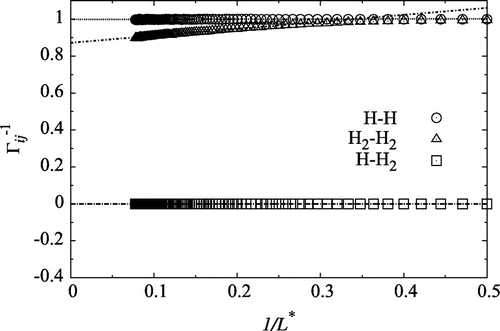
We shall present results in this article for a gas mixture of reduced density (0.0052 g cm). The thermodynamic correction factors obtained from particle fluctuations are plotted versus the inverse sphere size (1 / L) in Figure 1 at temperature (where ). The values in the region were fitted with straight lines, and extrapolated to the thermodynamic limit ( and ), the range where the linear 1 / L-dependence was observed. This range corresponds to spheres that include from 12 to 16 particles at this density and temperature. The value of obeys the ideal property already for a wide range of values, while increases from approximately 0.9 for the biggest sphere to 1 for . The correlation between H and H is near zero, explained by the dominating concentration of H. Only varies as a function of 1 / L, and the inverse thermodynamic factor increases with decreasing radius of the sampling sphere. See [12] for more details.

Figure 1. The inverse thermodynamic correction factor, for a mixture of atomic hydrogen and molecular hydrogen at density and . At this temperature, the degree of dissociation was independent of density within the numerical accuracy of the simulation. The straight lines were fitted in the region in order to find the value in the thermodynamic limit.

The partial enthalpy of component i, , at constant is determined from the following equation:(17)

Brackets denote time and/or ensemble averages. The partial enthalpies are also (predominantly) linear functions of the inverse of the radius of the small sampling volume (for spherical sampling volumes), L (see also [15–17,22]. The partial enthalpies of the small sampling volumes are related to the partial enthalpies in the thermodynamic limit through(18)

where is the partial enthalpy at constant in the thermodynamic limit.

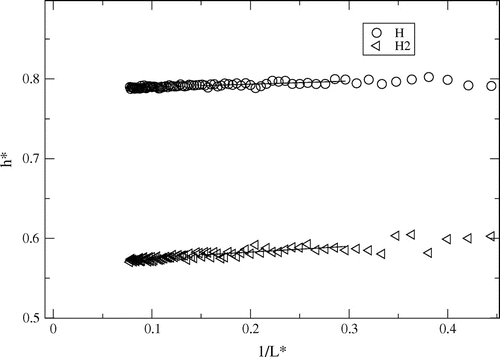
The partial enthalpy, , was determined for the small systems at constant (). The results for h for H and H are shown as a function of the inverse radius of the small system in Figure 2 for . At this temperature, the mole fraction of H varies from () to () between the lowest and the highest densities. Straight lines were fitted to in the range . This range was chosen after comparing results for systems with with 1000 and 4096 particles. No size effect was seen between these system. At the other temperatures, results also looked like Figure 2.

Figure 2. Partial enthalpies determined from fluctuations at (), , as a function of inverse sphere radius for reduced density 0.0003 at . Straight lines were fitted in the region .

3.3. Kirkwood–Buff integrals

In general, Kirkwood–Buff integrals, ,[27] can be used to find thermodynamic variables like thermodynamic factors, partial molar volumes or isothermal compressibility. This can be done by considering density fluctuations in the grand-canonical ensemble, or pair correlation functions.[28] is defined as the integral over the pair correlation function :(19)

where is the Kroenecker delta and is the concentration of i (). The last equality was obtained by introducing Equation (15(15) ) in the middle equality of Equation (19(19) ).

The derivative of the chemical potential of k is related to at constant T and P by:(20)

where is the mole fraction of i (; here is the number of molecules so that ). The relation between the thermodynamic correction factor and the activity coefficient, is then [17]:(21)

Other thermodynamic properties can also be defined in terms of these integrals. The fluctuation method gives access to values for the () ensemble. In order to refer to conditions that are interesting to chemists, these values must be transformed to the canonical () or isothermal–isobaric () ensemble. Such transformations can only be done in the thermodynamic limit, see Schnell et al. [22] for a detailed discussion.

4. The chemical reaction away from equilibrium

4.1. The entropy production and the flux equations

In our example, the chemical reaction takes place in a closed box exposed to a temperature difference in one direction, the x-direction. The temperature and chemical potentials vary only in this direction. In molecular dynamics simulations, the convenient flux variables are the total heat flux , the flux of hydrogen atoms and the flux of hydrogen molecules , in addition to the reaction rate r.

The simulations are set up with a gradient in temperature, and allowed to run until stationary state. Then(22)

and(23)

There is no net mass flux out of the box, so the two molar fluxes are dependent: .

The entropy production is then (see [18,20] for details):(24) (25)

The (scalar) chemical reaction rate r depends on the driving force in a non-linear way, cf. Equation (39(39) ). It will not couple to the vectorial fluxes (like heat and mass fluxes).[18] Practical flux expressions for and are obtained from the force–flux relations:(26) (27)

where the forces are written as a function of the resistivities, R, and the fluxes. Alternatively, we can write the fluxes as a function of the forces and the conductivities L as follows:(28) (29)

The coefficients R and L can be organised in a matrix of resistivities and conductivities, respectively. The resistivity matrix R has its inverse in the conductivity matrix L. Both matrices are symmetric.[29,30] The driving force in the last line should not be confused with the scalar driving force of a chemical reaction. It appears as a particular difference in the gradients of the chemical potentials, due to the relation between the fluxes, and therefore related to the reaction Gibbs energy. The driving force for interdiffusion of components is a vector; it is the gradient in the reaction Gibbs energy over temperature at any location x. This quantity does not change sign across the box, as we shall see. The value of the R- or L-matrix must be understood on this basis.

A formulation containing the total heat flux is not convenient when it comes to making a connection with experiments, as it is not absolute, but depends on a reference state for the enthalpy. The measurable heat flux, , is introduced via the total heat (or energy) flux :(30)

where was defined earlier. We obtain(31)

where subscript T indicates that the reaction Gibbs energy is now found while the temperature is kept constant. This form of the entropy production gives flux-force relations which relate directly to measurable quantities:(32) (33)

or, alternatively(34) (35)

The symmetric coefficient matrix of resistivities, r, is the inverse of the coefficient matrix of conductivities l. All sets of coefficients will be found and related to the more common coefficients of transport in the next subsection.

The entropy production must be invariant to the choice of variables. This gives the following relations between the resistivities:(36) (37) (38)

The non-linear flux–force relation of the chemical reactions can be derived using mesoscopic non-equilibrium thermodynamics.[31] This gives:(39)

The equation can be seen as a rewriting of the law of mass action.[31] From the law of mass action, we can set the forward reaction rate as of a pseudo-first-order reaction:(40)

where is the reaction coefficient. In equilibrium, . Knowing , we can calculate the reaction Gibbs energy at any location in the system from Equation (39(39) ):(41)

Close to chemical equilibrium, , and the reaction rate in Equation (39(39) ) becomes(42)

We see immediately that the net rate is zero when , near as well as far from chemical equilibrium, as expected.

4.2. Transport properties

In multicomponent systems with transport of heat and mass, one can define two thermal conductivities; one for the homogeneous mixture, and one for zero mass transport (Soret equilibrium).[31] The situation here is similar in the sense that we have zero net mass transport. But it is not the same, as the component fluxes differ from zero. We can define one conductivity for zero component fluxes, and one conductivity for a constant driving force for interdiffusion.

The thermal conductivity, , defined in the absence of component transport, is the normal thermal conductivity for momentum transfer. We obtain from Equation (34(34) ):(43)

This situation, with no movement of the chemical components cannot be realised in this simulation system. The quantity can nevertheless be computed.

The thermal conductivity at is defined from Equation (32(32) ):(44)

This conductivity is defined at a constant chemical driving force, . In the present case, the chemical reaction occurs everywhere in the box, and its driving force is not constant. The interdiffusion of components in the box contributes to heat transfer, and makes this thermal conductivity different from . According to non-equilibrium thermodynamics theory, the coefficients are independent of the driving forces,[18] so a value obtained for one driving force can be applied at any driving force.

The interdiffusion coefficient for movement of H vs. H, D, is defined by [20]:(45)

where the difference in the chemical potentials of H and H have been contracted by the help of the Gibbs–Duhem equation. The derivative of the chemical potential with respect to the density can be found from Equation (20(20) ).

The heat of transfer, is finally defined as the ratio between the measurable heat flux and the flux of H at zero temperature gradient:(46)

We will present all the above coefficients, calculated from the outcome of Equations (36(36) )–(38(38) ), once the matrix of L-coefficients is known.

4.2.1. Analytical solutions and procedure for decomposition of results

The derivatives of Equations (26(26) ) and (27(27) ) can, using Equations (22(22) ) and (23(23) ), be written in the form(47) (48)

Close to chemical equilibrium, we can use Equation (42(42) ) for the reaction rate,(49) (50)

When the rate constant and the resistivities are known and constant, these equations can be solved for given boundary conditions of the temperatures and mass fluxes, see Xu et al. [20].

The penetration length, d, is often used to characterise the competition between reaction and diffusion. We understand d as the distance a molecule can diffuse before it reacts:(51)

The solution of Equations (49(49) ) and (50(50) ) is for :(52) (53)

This results in the following expressions for the fluxes and the reaction rate(54) (55) (56)

where , , and are defined by(57) (58) (59)

The function giving the flux of H in Equation (55(55) ) approaches zero in and . The analytical expression predicts a solution to the profile of the mass flux which is symmetric around the centre of the box, and can be used for fitting data.

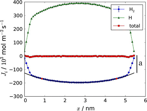
We fitted the simulation results for the hydrogen flux to the following equation:(60)

where a is a constant due to energy delivery and consequent shift of the reaction in the thermostatted layers, see the Simulation section below. We corrected the observed hydrogen flux for a, and fitted the central part of the curve to give a, and l / d.

Figure 3. Fluxes of hydrogen molecule, and atom, through the box. The total mass flux, , is constant as no net mass flux is present. The constant a, obtained from the fit, is indicated on the right side of the figure. The temperature gradient was created by velocity swapping (0.17 swaps/fs, with 85% success). See Section 5 for more details on the computational method.

With knowledge of l / d, we fitted the computed inverse temperature profile through the box to Equation (52(52) ), and determined , and (defined in Equations (57(57) )–(59(59) )). When is known, can be found from which was determined from the fit of .

The total heat flux, , can be found directly from the simulations, as explained in Section 5. The measurable heat flux, , can be found from the total heat flux using relation Equation (30(30) ). From knowledge of and , was determined using Equation (54(54) ). Finally, the l-matrix was found by inverting the r-matrix. Knowing , , and , we can find from Equation (28(28) ), and further from Equation (29(29) ) and .

From the L-matrix we found the R-matrix by inversion. The R-matrix was then used to determine the r-matrix, according to the relations given in Equations (36(36) )–(38(38) ), as well as the reaction enthalpy.

5. Molecular dynamics simulations

We report simulation results for a gas mixture of density 0.0052 g cm in the temperature range 3640–20.800 K. The simulation box contained 1000 particles (), with dimensions , where . The mass of one hydrogen atom,  kg, was used to define the reduced total mass density . This implies that the reduced total mass density is equal to the reduced total molar density in terms of (). Reduced units (see Table 1) are indicated by superscript .[11] In these units . The value of in the table was obtained at , giving . Due to the 3-particle interaction the excluded volume diameter is much larger, 2.7 Å. The was derived from the binding energy of hydrogen, so that is the minimum of the pair potential, giving 51991 K. For more details of the simulation procedure, see [11].

Table 1. Relations between reduced and real units. In this study 51991 K, and  kg.

Reduced variables	Formula
Mass
Distance
Energy
Time
Temperature
Density
Pressure
Velocity	vv

The temperature T of a volume element is calculated from the average kinetic energy per degree of freedom of all particles:(61)

where and is the total number of atoms.

In the small system method, one samples fluctuations in small spheres in the simulation box. The sphere had radius, L, varying from to , where is the length of the simulation box in the y-direction. The sampling is done at random positions in the simulation box. The number of particles and the energy is then computed for each sphere (50 spheres per sampling) and the time average gave the fluctuation of particle numbers and energy. Fluctuations were sampled every 100-time step.

The NEMD simulations reported here were run for 600 million steps (6 parallel runs of a 100 million steps, where 3 million steps were used for each parallel run to make the system stationary). The time step was in reduced units, corresponding to 0.02 fs. After a stationary state was reached, data were sampled every 20 steps.

We adopted the thermostatting routine from Müller-Plathe [32] to impose a thermal gradient. The simulation box is an elongated system, where the centre of the box is designated the cold zone, and the edges are designated the hot zone. This symmetry allows us to average the data from a simulation more efficiently. Two atoms were picked at random, one in the designated hot zone and one in the cold zone. Then the kinetic energy of the particles was swapped if the kinetic energy of the particle in the cold zone was higher than that of the particle in the hot zone. The frequency of the velocity swaps regulates the energy flow between the hot and cold zone, and thus also the observed temperature gradient. We determined a range of swapping conditions which produced the expected symmetry. An overview of the possible gradients produced by the various swapping conditions is presented in Table 2, for a temperature of 10,400 K in the centre of the transport region. However, the thermostatting routine leaves two zones on both side of the plots, e.g. Figure 3. This is due to the thermostat itself, and these regions should be excluded from the analysis.

From the energy change resulting from the swaps, we have the total energy flux:(62)

where v is the velocity and t the time over which the transfers were counted. The factor 2 in the denominator arises from the periodicity of the system, as the energy can flow from the hot to the cold slab from two directions (the cold zone is at the centre of the box, and the hot zone is at both ends to ensure symmetry). This effectively doubles the available area . In the x-direction, the simulation box was subdivided in 128 layers. The thermodynamic properties were calculated in each of these layers.

Table 2 presents an overview of the cases we studied. Cases 1a–1d have been performed around the same initial temperature, 10,400 K, but with varying temperature gradients (created by different swap frequencies). Six parallel runs with different initial configurations runs were done for each swap condition.

Table 2. The thermal gradient was found from the indicated points (red) in the temperature profile, see Figure . Cases 1a–1d have been performed for the same average temperature, 10,400 K. The success of the thermostat was measured by the number of successful velocity swaps that meet the energy criterion.

Case no.	T(l / 2)		dT/dx	Swap frequency	Success rate
	K	K		fs	%
1a	10.5	-1430	-3.9	0.17	85
1b	10.4	-1070	-2.9	0.13	87
1c	10.3	-940	-2.6	0.10	88
1d	10.4	-750	-2.2	0.08	89
2	15.7	-1210	-3.3	0.10	89

The energy fluxes used are shown in Table 3. The thermostat-dependent coefficient a (from the fit of the flux) was used to correct the mass flux, , and the total heat flux, , prior to further calculations. This helps remove the effect of the thermostats on the simulated results.

Table 3. The corrected total heat flux, , measurable heat flux, and the corrected mass flux , at (l / 2).

Case
	W m	W m	mol m
1
2

The average temperature in the simulation was (10400 K). At this temperature, the equilibrium composition contains a sizable concentration of product (H) as well as reactant (H), 50% dissociation, see [11], making it suitable for a study of the impact of the reaction on transport properties. Cases 1a–d, which have the same temperature in the centre of the box, will generate the same set of transport coefficients, as these are independent of the driving force. The average of the separate results will be referred to as Case 1 in the following.

6. The reaction in equilibrium

6.1. Mixture compositions

The degree of dissociation, mole fraction and pressure of the mixture are given in Table 4. We see that there is almost 1% dissociation at the lowest temperature (), while for the highest temperature (), we have almost 80% dissociation. The ideal dissociation constant is also calculated. The nearly ideal state at 3640 K () can be used as a reference.

Table 4. Number of H atoms (), mole fraction (), total pressure () and the dissociation constant () for the density, .

	0.07	0.15	0.2	0.25	0.3	0.4
	8	254	477	574	711	761
	496	373	261	213	145	120
	0.984	0.595	0.353	0.270	0.169	0.136
	–	0.276	1.183	1.973	4.088	5.502
	1.138	3.045	4.672	6.347	7.983	11.148

6.2. Thermodynamic correction factor

The inverse thermodynamic correction factor in the thermodynamic limit, , is plotted in Figure 4 as a function of temperature for the density in question. Open symbols correspond to , filled symbols to and crosses to .

Figure 4. The inverse thermodynamic correction factor in the thermodynamic limit, for the mass densities .

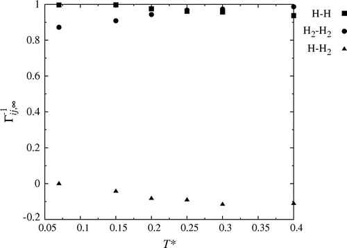
The figure shows that is approximately constant independent of temperature and density. A small decrease is seen with increasing temperature. An increasing temperature leads to an increasing amount of H in the system, see Table 4.

The value of is seen to increase with temperature, as the amount of H decreases. We see that it increases from approximately 0.9 to 1 in the investigated temperature interval. The temperature dependence is larger for denser mixtures (See [12]).

The value of the thermodynamic correction factor for one component interacting with itself is 1 if the system is ideal (pure component and ideal gas). The value is zero for interactions between different components in this state. We conclude that the gas at the lowest temperature, , is close to an ideal mixture. At these conditions, only 0.8% of the hydrogen is dissociated (8 H atoms out of a 1000 particles).

6.3. Partial enthalpies

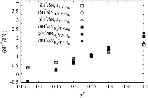
Results for the partial enthalpies in the different ensembles are presented for the temperature interval . See Ref. [22] for details. The partial enthalpies in the thermodynamic limit are given in Table 5. All results showed a linear dependence and the linear fit was done for the range   in all cases. The partial enthalpy in the table increases with increasing temperature, for H as well as H. All sets of partial enthalpies; for (), () and () are shown in Figure 5. The values obtained in the () ensemble are special in that they are designated partial molar enthalpies, and can be used to calculate the reaction enthalpy.

Table 5. Partial enthalpies, at , in the thermodynamic limit. Values are given in reduced units.

0.07	0.34	-0.46
0.15	0.60	0.18
0.2	0.79	0.57
0.25	0.98	0.95
0.3	1.19	1.31
0.4	1.59	2.04

Figure 5. Partial enthalpy in the ensembles; , and . Open symbols corresponds to values for H, while closed symbols represent H.

6.4. The reaction enthalpy and the equilibrium constant

6.4.1. The standard state. Pressure variations of the reaction enthalpy

In order to determine the thermodynamic equilibrium constant from the van’t Hoff equation, Equation (11(11) ), we need information on the standard state, in the present case defined by an ideal gas at 1 bar. The lowest density mixture of reactant and product is close to be an ideal mixture, because the thermodynamic correction factors for the main components are close to unity at this condition, , , and . In addition, the compressibility was near 1 / P, the ideal value.

We find an ideal standard state from results at the lowest temperature, (), and use Equation (13(13) ) to correct for the distance to 1 bar. At this temperature and density, the overall pressure of the system is approximately 850 bar. The pressure variation from 1 bar to 850 bar gives a contribution of 7 units to which must be added to the normal van’t Hoff term, see Equation (13(13) ) for these conditions. For the whole range of pressures and densities used, the correction term varies from 3–24 units. The enthalpy of reaction was observed to only have a small pressure dependence. The enthalpy of the reaction was observed to follow a quadratic trend as a function of temperature.

6.4.2. The temperature dependence of the enthalpy

Figure 6. Reaction enthalpy, , as a function of temperature. The points () represent results the simulation, where . The polynomial line represents the fit of the reaction enthalpy to a temperature function. The straight line represents the constant ideal result [11] found by plotting as a function of temperature (1 / T).

Table 6. and as a function of the temperature.

0.15	604	628	1.0
0.2	3208	4126	0.8
0.25	8606	9344	0.9
0.3	16564	24356	0.7
0.4	37932	45778	0.8

From the results of the equilibrium simulations, we can include the temperature dependence of the enthalpy in the van’t Hoff equation. The variation in with temperature is given in Figure 6. The line in the plot corresponds to the value found for ideal conditions (plot of vs 1/T).[11]

The reaction enthalpy (in J mol) was fitted to a quadratic function of the temperature:(63)

We rewrite the van’t Hoff equation, using the identity , , and obtain after integration:(64)

The thermodynamic equilibrium constant and the ratio of the activity coefficients calculated from this equation and Equation 11(11) are shown Table 6. When we include the temperature dependence in , we obtain in the same order of magnitude as and , see Table 6. The ratio of the activity coefficients is not constant and follows the same temperature dependence as we observe for . From the approximation   in the last term in Equation (13(13) ), we calculate a negligible correction due to the pressure variation in of 3–24 units, varying from the lowest to the highest temperature.

6.5. Equilibrium simulations – summarised

We have seen above how the small system method can be used to give accurate data for chemical reactions. It may seem cumbersome to have to transform variables between ensembles, but the transformation procedure is well established.[22,33] The bonus is that information can be obtained about non-ideal behaviour in mixtures and chemical reactions. This information is otherwise not easily accessible.

The results elucidate that the normal assumption of taking the reaction enthalpy constant in the integration of the van’t Hoff equation can be significantly improved, see Figure 6. The calculated reaction enthalpy has the same order of magnitude (440 kJ mol) as the bond dissipation energy in the interaction potential (432 kJ mol). The large value may change the transport properties of the mixture, and it is important to know it precisely.

7. The reaction away from equilibrium

7.1. A stationary state of thermal interdiffusion

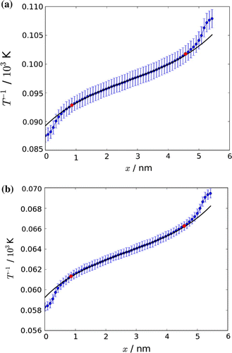
The main force driving transport in our box is the gradient in the inverse temperature. The inverse temperature is illustrated in Figure 7 for Cases 1c and 2. The figure shows the average of six parallel runs for each case. The variation in the inverse temperature was fitted to Equation (52(52) ). Error bars indicate the variation between the runs. The accuracy of the fit is slightly better for Case 1 (Figure 7(a)) than for Case 2 (Figure 7(b)).

Figure 7. The average of six runs of an inverse temperature profile through the box. Error bars are shown. The inverse temperature profile was fitted, according to procedures described in the text, to (Equation (52(52) )). The red markers indicate the start and stop of the fit.

The thermal gradient leads in both cases to an interesting stationary state, which was shown already in Figure 3. The two components, which are confined to the box, diffuse due to the thermal gradient. The hydrogen atoms diffuse to the cold side of the box, while the hydrogen molecules diffuse to the warm side, giving rise to thermal interdiffusion.

The average mass fluxes of the molecules and atoms were determined from six parallel runs at two temperatures (not shown). The net mass flux () through the system was always zero, as it should be, confirming the relation . An increase in the temperature increased the component fluxes as the driving force was increased.

In a non-reacting mixture of two components, this interdiffusion is absent. The observed thermal interdiffusion of components has therefore its origin in the chemical reaction. We see a variation in the particle fluxes across the box. This is another indication of an impact of the chemical reaction, as the divergence of the flux is related to the reaction rate, see Equation (22(22) ). Chemical reactions at equilibrium are shifted with the temperature according to Le Chatelier’s principle. In this case, we are far from chemical equilibrium in the ends of the box. We find an increase in the number of molecules at low temperatures. This can be said to be in agreement with Le Chatelier’s principle. But, it contains an extra element, since we do not compare equilibrium states. When the net reaction leads to release of heat by shifting to the side of the molecule, there is also an extra delivery of heat to the heat sink (the cold zone). There is thus an additional mechanism of heat transfer due to the chemical reaction, supplementing the ordinary mechanism of momentum transfer.

The increase in the mole fraction of hydrogen molecules on the low-temperature side, on the cost of the mole fraction of the hydrogen atom, is shown in Figure 8. The shifts through the box are in agreement with the direction of component fluxes in Figure 3, as well as the distribution of components through the box.

One may say that the non-equilibrium stationary state is characterised by a dissipative structure maintained by energy supplied from the outside. Seen from the outside, the simulation box appears as a medium for heat transfer only. The entropy production can therefore also be expressed by the energy flux times the thermal driving force. The more detailed picture used here, offers an explanation of the causes of dissipation and the mechanism for heat transfer.

Figure 8. Mole fraction of H and H, , along the simulation box (a), and measurable heat flux, , with the reaction enthalpy carried by the molecule, , along the simulation box (b).

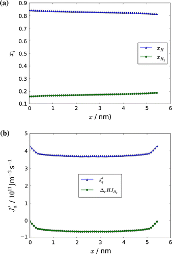
The total heat or energy flux is constant through the box according to Equation (23(23) ) and is known from the simulation. The contributions to the energy flux from the measurable heat flux and from the reaction enthalpy times the flux of molecules are shown in Figure 8. At the boundaries x(0) and x(l) the measurable heat flux is equal to the total heat flux, as the contribution from the mass flux goes to zero, as can be seen from Figure . The pressure through the box [11] was always constant within the accuracy of the calculation as expected (not shown).

7.2. Properties of the chemical reaction

The flux of molecular hydrogen was first fitted to Equation (60(60) ), using the procedure described above. The constants from the fit are shown in Table 7. The parameter l / d was obtained in this fit. From knowledge of l / d and the results of the fits of the analytical curves to the inverse temperature profile, we computed the constants and , see Table 8. On the basis of these results, we computed the various sets of phenomenological coefficients, as described earlier in the text. Similar data for fluorine [20] did not have the accuracy to do so.

Table 7. Constants from fit to mass flux according to procedures described in the text. Case 1 is the average of Cases 1a–d.

Case			l / d
	mol m s	mol m s	–
1
2

Table 8. Constants obtained from the fit of the inverse temperature profile, as described in the text. Case 1 is an average of Cases 1a–d.

Case
	K	K m	K
1
2

Table 9 presents the penetration depth, d, of the hydrogen dissociation reaction, e.g. how far a particle can diffuse before it reacts. The average value obtained for Case 1 is , and for Case 2, see Table 9. A reduction in d with temperature is likely. For comparison, the mean free path of a hydrogen atom, , at the given density is , as calculated from the total volume of the box, the excluded diameter found from the pair correlation function (, see [11]) and the total number of particles (). We conclude that the reaction in the present case is very fast and that particles will react after the first or second collision with another particle. Xu et al. [20] found a smaller penetration depth, for fluorine. Their reaction was less endothermic 200 KJ mol compared to about 424 KJ mol in the present case.

Table 9. Forward rate constant, , penetration depth, d, and mean free path of hydrogen, . Case 1 is an average of case 1a–d

Case		d
	m mol
1			10
2			10

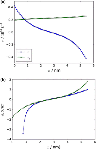
The net rate, r from Equation (22(22) ), and the forward rate, , are plotted in Figure 9. From the figure, we see that the forward rate is larger than the net rate through the box, except in the hot region, where the net reaction goes in the opposite direction. The corresponding chemical driving force, from Equation (53(53) ), is plotted in Figure 9. We see that only in the centre of the box, . We approach chemical equilibrium near the centre. In general, we are far from equilibrium in most of the box, where is in the order of several thousand kJ mol. Peculiar is the shift in sign of the driving force and the net rate, taking place in the centre. This means that the reaction is actively and rapidly absorbing heat on the hot side and actively delivering heat on the cold side. The large value and the sign of the reaction rate must explain much of the mechanism for heat transfer.

The ratio was found from the net and the forward rate according to Equation (41(41) ), and the result of this calculation is included in Figure 9 (circles). We see that the two curves are crossing zero on the same location in the box. This is necessary, as the rate is zero when the driving force is zero. It is interesting that the approximate expression used by Xu et al. [20] overlaps with the analytical expression used here, in the centre of the box. The earlier and the present analysis are thus supporting each other, when we approach conditions near equilibrium.

Figure 9. (a) The variation in the net reaction rate, r, and the forward reaction rate, (b), and in the dimensionless chemical driving force through the box. The approximate expression Equation (42(42) ) to the driving force is also shown in Figure (b).

7.3. The transport coefficients for heat and mass

We can finally return to the issue of transport coefficients for heat and mass in the reacting mixture. The various sets of phenomenological coefficients obtained from the parameters in Tables 7 and 8 are shown in Tables 10 and 11. As mentioned before, uppercase symbols for the coefficients refer to the description with the energy flux as a variable, lowercase symbols for the coefficients refer to the description using instead the measurable heat flux as a variable.

We first checked that all sets of resistivities and conductivities had a positive matrix determinant. This is required from the second law of thermodynamics. We verified furthermore that Cases 1a–d gave the same coefficients within the accuracy of the simulation (not shown). This is also required in non-equilibrium thermodynamics; coefficients do not depend on the driving force. We proceed with the average of these values which defined Case 1.

Table 10. Resistivities to transport of heat and mass for various sets of fluxes and forces (see text for definitions).

	m W K	ms mol K	J ms mol K	m s mol K	J ms mol K
1
2

Table 11. Conductivities for transport of heat and mass for various sets of fluxes and forces (see text for definitions).

	W K m	mol K m s	mol K,J ms	W K m	mol K m s
1
2

To the best of our knowledge, the full set of coefficients for a reacting gas mixture have only been estimated once before, by Xu et al. [20]. The thermal resistivities, , are in the same order of magnitude in the two investigations, but the resistivities to mass transfer are one order of magnitude larger in the present case, where the reaction enthalpy is larger and the particles smaller in size. The coupling coefficient, , is also one order of magnitude larger in the present investigation. The sign of is positive for hydrogen dissociation, while it was negative for fluorine association.[20] The choice of a positive direction for the reaction explains the sign of the coefficient, cf. Equation (37(37) ). In a situation, with lack of data to compare with, it is good to know that system behaves according to predictions from theory.

We calculated also the more familiar transport coefficients, as defined by Equations (43(43) ) () and (45(45) ) (). The results for these transport coefficients are shown in Tables 12 and 13. The local temperature was used to find the interdiffusion coefficient, see Equation (45(45) ), meaning that it varies across the box. There is also a small contribution from the non-ideality of the mixture, from the derivative . The value is decisive for the observed interdiffusion.

Butler and Brokaw [34] related the binary diffusion coefficient, , of a reacting mixture to the enthalpy of reaction and the thermal conductivity:(65)

Here, is the thermal conductivity in the presence of a chemical reaction, is the mass fraction of component i and n the stoichiometric constant. As a measure for , we take our value of . The result is also shown in Table 12

Table 12. The interdiffusion constant, from simulations () and kinetic theory () in the centre of the gradient (at l / 2) and the binary diffusion coefficient, , according to Butler and Brokaw [34]. All units are in m s.

Case
2

As can be seen from Table 12, the interdiffusion coefficient from the simulations is two order of magnitudes smaller than the value found using Equation (65(65) ) from kinetic theory. The main contribution to comes from , which is one order of magnitude smaller than obtained by Xu for fluorine.[20]

The thermal conductivities, and , are derived from and , respectively. The values in Table 13 for are as expected for a gas at high temperature.[35] In this case, kinetic theory gives 1.3 , comparable to the results for . But, striking is that the value of , for which there is no comparable data, is up to 5 times larger than the value of . Butler and Brokaw [34] observed a similar trend in their estimates for thermal conductivities of dissociative reactions, from a different basis, however. The result shows that the chemically reacting mixture is much more able to conduct heat, than a non-reacting mixture. In a search for well-conductive fluids, this finding may be interesting. It is unfortunately not yet possible to discuss how general the finding is, for instance whether or not it is related to distance of the reaction from chemical equilibrium. This should be studied further.

Table 13. Heat of transfer, , and the thermal conductivities in the absence, and presence, (from ), of a chemical reaction. The reaction enthalpy, 424 kJ mol, refer to the average temperature in Case 1.[11]

Case
	kJ mol	W K m	W K m
1
2

The transport property that expresses the coupling between the heat and mass flux, the heat of transfer, is also presented in Table 13. The negative sign means that heat is transferred in the direction opposite to the movement of the molecule. Extra heat is thus transported down the temperature gradient. Surprising is the high value of the heat of transfer. Common values for heats of transfer are typically some kJ. Near chemical equilibrium Xu et al. found ,[20] giving a value of several hundred kJ. Our value is up to 10 times higher than the enthalpy of reaction. The interdiffusive fluxes are without doubt effective as contributors to the mechanism of heat transfer. The small penetration depth, the large enthalpy of reaction and the large reaction rate are also likely to play a role. Clearly it is not a valid assumption to neglect the coupling of heat and mass (a Dufour-type contribution), in the description of heat transport in a chemically reacting mixture. Therefore, more research is needed to obtain a more precise picture and insight into this unexplored territory.

8. Conclusions

For the first time, we have been able to decompose molecular dynamics simulation results of a chemically reacting mixture and determine transport properties of the mixture without making assumptions of ideality; see also [11–13]. For the reaction this study has focused on, the hydrogen dissociation reaction, the chemical reaction in the closed box exposed to a thermal field is very far from chemical equilibrium away from the centre of the box. The thermal conductivity calculated from the measurable heat flux at a constant chemical driving force, is much larger than in a system without mass movement, while the diffusion constant is smaller than typical for gases. The heat of transfer is, however, very large, indicating that the mechanism of heat transfer changes radically in the presence of a reaction. The findings question the neglect of Dufour effects in the modelling of similar systems, and asks for systematic investigations.

As new force fields become available for calculation of chemical reactions using classical potentials, such as ReaxFF,[36] one may be able to use the procedure for more important chemical reactions.

Additional information

Funding

RS and SK are grateful to Storforsk Project Transport nr. [167336] from NFR and the Department of Chemistry, NTNU, for financial support. SKS was financially supported from the Research Council of Norway through a Post-Doc. Fellowship [grant number 230534].

Notes

No potential conflict of interest was reported by the authors.

References

- Fogler HS . Elements of chemical reaction engineering. Boston, MA: Prentice Hall International; 2006.
- Saumon D , Chabrier G . Fluid hydrogen at high density: the plasma phase transition. Phys. Rev. Lett. 1989;62:2397–2400.
- Sawada K , Fujimoto T . Effective ionization and dissociation rate coefficients of molecular hydrogen in plasma. J. Appl. Phys. 1995;78:2913–2924.
- Magro WR , Ceperley DM , Pierleoni C , et al . Molecular dissociation in hot, dense hydrogen. Phys. Rev. Lett. 1996;76:1240–1243.
- Ward TL , Dao T . Model of hydrogen permeation behavior in palladium membranes. J. Mem. Sci. 1999;153:211–231.
- Skorpa R , Voldsund M , Takla M , et al . Assessing the coupled heat and mass transport of hydrogen through a palladium membrane. J. Mem. Sci. 2012;394--395:131–139.
- Langmuir I . The dissociation of hydrogen into atoms. J. Am. Chem. Soc. 1912;34:860–877.
- Lide DR . CRC handbook of chemistry and physics. 85th ed. Boca Raton: CRC Press; 2004.
- Holleman AF , Wiberg E , Wiberg N . Inorganic chemistry. San Diego, CA: Academic Press; 2001.
- Kohen D , Tully JC , Stillinger FH . Modeling the interaction of hydrogen with silicon surfaces. Surface Sci. 1998;397:225–236.
- Skorpa R , Simon J-M , Bedeaux D , et al . Equilibrium properties of the reaction {H}{H}. Phys. Chem. Chem. Phys. 2013;6:1227–1237.
- Skorpa R , Simon JM , Bedeaux D , et al . The reaction enthalpy of hydrogen dissociation calculated with the small system method from simulation of molecular fluctuations. Phys. Chem. Chem. Phys. 2015;16:19681–19693.
- Skorpa R , Vlugt TJH , Bedeaux D , et al . Diffusion of heat and mass in a chemically reacting mixture away from equilibrium. J. Phys. Chem. C. 2015;119:12838–12847.
- Hafskjold B , Ikeshoji T . Partial specific quantities computed by nonequilibrium molecular dynamics. Fluid Phase Equilib. 1995;104:173–184.
- Schnell SK , Vlugt TJH , Simon JM , et al . Thermodynamics of small systems embedded in a reservoir: a detailed analysis of finite size effects. Mol. Phys. 2012;110:1069–1079.
- Schnell SK , Vlugt TJH , Simon J-M , et al . Thermodynamics of a small system in a reservoir. Chem. Phys. Lett. 2011;504:199–201.
- Schnell SK , Liu X , Simon J-M , et al . Calculating thermodynamic properties from fluctuations at small scales. J. Phys. Chem. B. 2011;115:10911–10918.
- de Groot SR , Mazur P . Non-equilibrium thermodynamics. New York (NY): Dover Publications; 1984.
- Xu J , Kjelstrup S , Bedeaux D . Molecular dynamics simulations of a chemical reaction; conditions for local equilibrium in a temperature gradient. Phys. Chem. Chem. Phys. 2006;8:2017–2027.
- Xu J , Kjelstrup S , Bedeaux D , et al . Transport properties of 2{F}{F} in a temperature gradient as studied by molecular dynamics simulations. Phys. Chem. Chem. Phys. 2007;9:969–981.
- Xu J , Kjelstrup S , Bedeaux D , et al . The heat of transfer in a chemical reaction at equilibrium. J. Non-Equilibr. Thermodyn. 2007;32:341–349.
- Schnell SK , Skorpa R , Bedeaux D , et al . Partial molar enthalpies and partial molar reaction enthalpies from equilibrium molecular dynamics simulation. J. Chem. Phys. 2014;141:144501.
- Stillinger FH , Weber TA . Molecular dynamics simulation for chemically reactive substances. fluorine. J. Chem. Phys. 1988;8:5123–5133.
- Diedrich DL , Anderson JB . An accurate quantum Monte Carlo calculation of the barrier height for the reaction H +H = H + H. Science. 1992;258:786–788.
- Diedrich DL , Anderson JB . Exact quantum Monte Carlo calculations of the potential energy surface for the reaction H +H H + H. J. Chem. Phys. 1994;100:8089–8095.
- Reed DA , Erlich G . Surface diffusion, atomic jump rates and thermodynamics. Surface Sci. 1981;102:588–609.
- Kirkwood JG , Buff FP . The statistical mechanical theory of solutions. I. J. Chem. Phys. 1951;19:774–778.
- Krüger P , Schnell SK , Bedeaux D , et al . Kirkwood-Buff integrals for finite volumes. 2013;4:235–238.
- Onsager L . Reciprocal relations in irreversible processes. I. Phys. Rev. 1931;37:405–426.
- Onsager L . Reciprocal relations in irreversible processes. II. Phys. Rev. 1931;38:2265–2279.
- Kjelstrup S , Bedeaux D . Non-equilibrium thermodynamics for engineers. Singapore: World Scientific; 2010.
- Müller-Plathe F . A simple nonequilibrium molecular dynamics method for calculating the thermal conductivity. J. Chem. Phys. 1997;106:6082–6085.
- Ben-Naim A . A molecular theory of solutions. Oxford: Oxford University Press; 2006.
- Butler JN , Brokaw RS . Thermal conductivity of gas mixtures in chemical equilibrium. J. Chem. Phys. 1957;26:1636–1643.
- Uribe FJ , Mason EA , Kestin J . Thermal conductivity of nine polyatomic gasses at low density. J. Phys. Chem. Ref. Data. 1990;19:1123–1137.
- van Duin ACT , Dasgupta S , Lorant F , et al . Reaxff: a reactive force field for hydrocarbons. J. Phys. Chem. A. 2001;105:9396–9409.