iRASPA: GPU-accelerated visualization software for materials scientists

Abstract

A new macOS software package, iRASPA, for visualisation and editing of materials is presented. iRASPA is a document-based app that manages multiple documents with each document containing a unique set of data that is stored in a file located either in the application sandbox or in iCloud drive. The latter allows collaboration on a shared document (on High Sierra). A document contains a gallery of projects that show off the main features, a CloudKit-based access to the CoRE MOF database (approximately 8000 structures), and local projects of the user. Each project contains a scene of one or more structures that can initially be read from CIF, PDB or XYZ-files, or made from scratch. Main features of iRASPA are: structure creation and editing, pictures and movies, ambient occlusion and high-dynamic range rendering, collage of structures, (transparent) adsorption surfaces, cell replicas and supercells, symmetry operations like space group and primitive cell detection, screening of structures using user-defined predicates, and GPU-computation of helium void fraction and surface areas in a matter of seconds. Leveraging the latest graphics technologies like Metal, iRASPA can render hundreds of thousands of atoms (including ambient occlusion) with stunning performance. The software is freely available from the Mac App Store.

Keywords:

• iRASPA
• molecular visualisation
• software
• crystallography

1. Introduction

Molecular simulation is a powerful tool to conduct ‘in-silico’ experiments on atomic systems. Density Functional Theory (DFT) is currently applicable to hundreds of atoms, but using a classical formulation trillions of atoms can be used [1]. However, while the increase in computational power and algorithms enable simulation of larger systems that can be run for longer times, one simulation itself is just one typical reproduction of the physics. To really get to the bottom of the physical, chemical and biological phenomena that occur, it is vital to elucidate the what, why and hows. Therefore, even if you could atomically simulate the system on large space and time-scales, in many cases it is preferable to simplify the system significantly to focus on one particular aspect. For example, using transition state theory for rare events, the reaction coordinate provides valuable information what exactly happens during the transition and why it occurs. Simulation methodology is not only to make simulations more efficient, but rather it usually provides additional information that is hard to obtain otherwise. Recently, we have made our advanced Monte Carlo code called ‘RASPA’ open source [2]. This software packages is well suited for simulating adsorption and diffusion of molecules in flexible nanoporous materials and to obtain molecular level information on these systems.

In this paper we present the second part, iRASPA, a macOS visualisation app for material scientists. Visualisation is another crucial tool for obtaining molecular level insight. Staring at the atomic positions in a CIF- or PDB-file for a long time will not get you closer to understanding the molecular structure. That is the job of ‘molecular visualizers’: to transform the data for efficient perception by the human brain. The human brain does not like tables of data, it likes graphs and plots, and from these we visually observe trends, patterns, relationships and exceptions. Here, we present a visualisation package aimed at material science. Examples of materials are metals, metal-oxides, ceramics, biomaterials, zeolites, clays and metal-organic frameworks (MOFs). For porous structures, like zeolites and MOFs, sometimes it is more useful to visualise the pores of the structures, rather than the atoms. That allows easy assessment of network topology, connectivity and identification of possible bottle-necks for diffusion. A static analysis of the energy landscape inside the pores allows examination of locations of large attractive interactions with the framework, which are prime candidates for adsorption and catalytic sites. Zeolites and MOFs are usually reported with a unit cell and a space group in CIF-file format [3]. It is very useful to be able to play around with creating supercells and symmetry operations.

Kozlikova et al. reviewed the state of the art of visualisation of biomolecular structures [4]. Some examples of molecular viewers are pyMol [5], VMD [6], Chimera [7], JMOL [8], Mercury [9], RASMOL [10], Materials Studio [11], Crystalmaker [12], Avogadro [13], VESTA [14], cellVIEW [15], MegaMol [16], and Qutemol [17]. Most visualisation packages are cross-platform. iRASPA is exclusively for macOS (starting from 10.11 El Capitan) and as such can leverage the latest visualisation technologies with stunning performance. iRASPA extensively utilises GPU computing [18]. For example, void-fractions andsurface areas can be computed in a fraction of a second for small/medium structures and in a few seconds for very large unit cells. It can handle large structures (hundreds of thousands of atoms), including ambient occlusion, with high frame rates.

The Metal framework provides near-direct access to the graphics processing unit (GPU) and optimised for the hardware available in Apple devices. It will in time replace OpenGL [19–21] and OpenCL [22–26], but these are still available as legacy/fall-back option. All Apple hardware sold from 2012 onward supports Metal. Metal is designed very well and arguably the most user-friendly next-generation graphical and compute application programming interface (API) available.

Modern mac apps are based on Cocoa [27–29] and written using the Xcode Integrated Development Environment (IDE) [30]. iRASPA is written in Swift 4.0 [31], with over 100.000 lines of code. It is heavily multi-threaded, by making use of Grand Central Dispatch (GCD) [32], to avoid blocking the user interface when doing computational intensive operations. Apple’s Core Animation infrastructure provides a general purpose system for animations. For example, when changing tabs the transitions cross-fade, reordering a table view is animated, drag and drop animations animate an opened gap for newly inserted items, and the atomic selection can be made to ‘blink’ (can be turned on and off in the user preferences).

iRASPA is different in philosophy from other existing software packages. It is document-based, which groups all your structures into a single document and allows collaboration using shared documents. On macOS High Sierra, you can place your document in ‘iCloud Drive’ and invite someone to collaborate on that document. iRASPA contains the CoRE MOF database [33,34] and zeolites IZA structures [35], stored in iCloud. The IZA (International Zeolite Association) Structure Commission is the authority to assign framework type codes (consisting of three capital letters) to all unique and confirmed framework topologies. Over 232 Framework Type Codes have been assigned to date. The CoRE MOF database contains approximately 8000 structures [33]. All the structures can be screened (in real-time) using user-defined predicates. The cloud structures can be queried for surface areas, void fraction and other pore structure properties.

iRASPA is available free of charge from the Mac App Store, the safest and easiest way to install apps on macOS. In the remainder we describe in Section 2 the capabilities of iRASPA in detail, with typical use-cases illustrated in Section 3. In the Appendix 1, we detail the visualisation technologies used in the implementation and in the Appendix 2 the algorithms for symmetry operations. We think this will be useful for readers interested in developing similar packages and serves as a review and summary of the literature.

2. Overview of iRASPA

iRASPA is a ‘document-based’ app managing ‘documents’. Conceptually, a document is a container for a body of information that can be named and stored in a file, locally and in iCloud. Document-based apps handle multiple documents, each in its own window, and often display more than one document at a time. In macOS Sierra or higher, apps can merge multiple windows into a row of tabs. To combine an app’s open windows into single window with tabs, choose Window > Merge All Windows. Document-based app offer many benefits: integration with iCloud storage, background writing and reading of document data, saveless model (autosaving), safe saving, version conflict handling and multilevel undo support.

2.1. Main interface

The main interface of iRASPA is a master-detail view. In a master-detail interface, the user can select projects from a list of projects and inspect the selected project. The master interface displays the collection of projects, and the detail interface implements an inspector of the selected project. Whenever the user changes the selection in the master interface, the detail interface is updated to show the new selection. If no project is selected, the detail interface displays nothing.

Figure 1. (Colour online) In a master-detail interface, changes in the primary view controller (the master project-view) drive changes in a secondary view controller (the detail views: render-, detail-, python- and log-views).

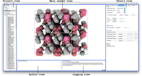
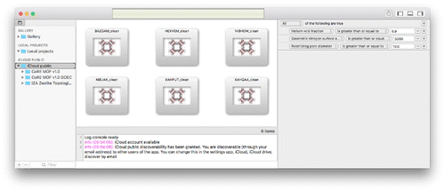
The main interface is shown in Figure 1. The project-view (project navigator) is the master that drives changes of the secondary views. The project-navigator has three sections: ‘GALLERY’, ‘LOCAL PROJECTS’ and ‘ICLOUD PUBLIC’. The gallery contains some examples to play around with. In ‘LOCAL PROJECTS’ you can store your own projects with editing capability, and the icloud-part contains cloud-stored databases. The ‘GALLERY’ and ‘ICLOUD PUBLIC’ sections are immutable, but can be dragged and dropped or copy-and-pasted to your ‘LOCAL PROJECTS’-section, after which they can be edited for content and appearance.

You can view and edit your own structures by importing them. The most common formats for structures are CIF-files [3] and PDB-files [36]. The easiest way of importing these types of files is to drag them from the Finder and then drop them in the project-navigator in the ‘LOCAL PROJECTS’-section. Alternatively, you can use the menu options +File > Import+.

The secondary views differ depending on the type of the selected project. Structures are viewed in a render-view with accompanying detail-view, python-view and log-view. In the detail-views, the atom and bond data are accessible in tabular form. The detail-view, the project-view and the python/log-view can be collapsed/uncollapsed using the show/hide toggles in the top-right part of the toolbar. In addition, a full screen mode is available using View > Enter Full Screen.

2.2. Render-view coordinate system and mouse controls

The chosen default coordinate system for the render-view is right-handed: the positive x and y axes point right and up, and the z points toward the viewer. This choice is consistent with most math and physics text books. Positive rotation is counterclockwise about the axis of rotation.

The mouse control is implemented as a ‘virtual trackball’ behavior which allows the user to define 3D rotation using mouse operations in a 2D window. The trackball works by assuming that a sphere encloses the 3D view. The user rolls this virtual sphere with the mouse. For example, if you click on the center of the sphere and move the mouse straight to the right, you rotate the scene around the y-axis. Clicking more towards the left edge of the centre and move the mouse straight to the right, you rotate the scene around the y-axis with a higher speed. You can click on the ‘edge’ of the sphere and roll it around in a circle to get a z-axis rotation. The trackball uses quaternions under the hood (Euler angles are less convenient due to gimbal lock problems) [37]. The mouse behaviour (with key-modifiers) is listed in Table 1.

Table 1. Basic mouse and keyboard event definitions for interactive use.

Mouse drag left/right	Rotate the scene left/right
Mouse drag up/down	Rotate the scene up/down
Right mouse click	Context menu
alt + right-mouse drag	Pan the structure
Mouse scroll-wheel or pinch gesture	Zoom in and out
Mouse click background	Unselect all
Mouse click object	Select the object
cmd + mouse click unselect object	Add object to selection
cmd + mouse click selected object	Remove object from selection
cmd + mouse drag	Add object in rectangular area to selection
shift + mouse drag	Replace selection by objects in rectangular area
alt + left mouse click background	Clear/reset measurement
alt + left mouse clicking on atoms 1 and 2	Distance measurement
alt + left mouse clicking on atoms 1, 2 and 3	Angle measurement
alt + left mouse clicking on atoms 1, 2, 3 and 4	Dihedral angle measurement
Mouse hoovering over object	shows tooltip

2.3. Selection, editing and measurement

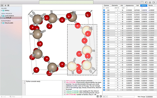
Selection and picking are integral parts of structure editing. Mouse picking means that the user clicks an object in the scene to select it, or interact with it otherwise. iRASPA provides pixel-perfect mouse picking for objects and area-selection. The selection of the render-view is in sync with the selection of the data-views in tabular form (see Figure 2). For individual picking, mouse-clicking an object selects it. If the modifier key @cmd@ is used, then the object is added to the selection. If that atom was already selected, it would be deselected (‘toggling’). In the render-view, the user can select a rectangular screen-area using the modifier key @cmd + dragging@ to add the atoms in that frustum to the selection, or use the modifier key @shift + dragging@ to replace the selection. In the data-views, the individual properties (e.g. position and charge) of atoms can be edited. Note that the atom list can be reordered and grouped together (the ‘outline-view’ is a type of table which lets the user expand or collapse rows that contain hierarchical data).

Figure 2. (Colour online) Editing structures and atomic selection using (i) the render-view or (ii) via the data-view, i.e. the atom-positions in tabular form.

2.4. Adsorption surfaces

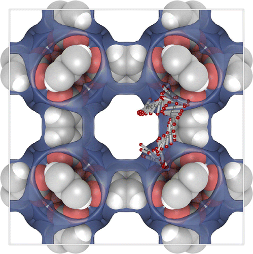
Examining the atomic positions of a molecular structure does not immediately lead to a thorough understanding of the structure. Molecular Shape Surfaces and Molecular Surface Maps [38] are used as a visual summarisation of a molecule’s interface with its environment. For crystalline, periodic nanoporous materials we use adsorption surfaces. Snurr et al. [39], at the advent of computational zeolite research, already used visualisation of energy contour plots and 3D density distributions of benzene in silicalite to obtain siting information. Dubbeldam et al. generated three-dimensional energy landscapes using the free energy obtained from the Widom insertion method [40]. One would like to know the details of the topology of the structure, and using iRASPA we can interpret and classify the structure by computing adsorption surfaces. Note that this analysis also immediately reveals ‘pockets’ that are not accessible from the main channel systems for the probe molecule.

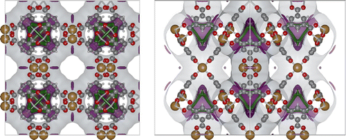
Figure 3. (Colour online) The atomic positions of two unit cells of the CHA-type zeolite, and the energy surface at three different values. CHA has (for helium) small inaccessible pockets located at (0,0,0).

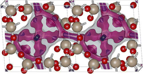
Figure 3 shows two unit cells of the atomic structure of the CHA-type zeolite along with three isosurfaces of helium at different energies: (1) energy zero to show the shape of the pores (transparent grey colour), (2) medium low energy to show the ‘diffusion paths’ (transparent magenta colour), and (3) the lowest energy sites that correspond to adsorption sites (solid blue colour). CHA has (for helium) small inaccessible pockets located at (0,0,0).

2.5. Ambient occlusion

‘Ambient occlusion’ is the shadowing of ambient light [41]. In geometric-based rendering, the illumination model is local. Ambient occlusion approximates the real-life radiation of light by producing effects like contact shadows that are unattainable in the standard local lighting model. Ambient occlusion is amongst the most powerful methods to improve depth perception, i.e. it darkens areas of the objects that light cannot access, therefore giving a much better perception of the 3D appearance. To give users the best experience when visualising molecular structures, ambient occlusion and shadowing methods should be included into molecular graphics packages to enhance user interaction with the structure. Advanced, yet efficient, lighting techniques including ambient occlusion, and hard and soft shadows, are key to improving the realism of the molecular visualisation [42]. Figure 4 shows an ionic-liquid system comparing standard VDW rendering versus adding ambient occlusion. Ambient occlusion drastically improves the perception of depth.

Figure 4. (Colour online) Ambient occlusion is computed per scene, (left) the water, cations and anions in the ionic liquid do not see each other, (right) the cations and anions occlude each other. The water is treated separately and drawn in ball-and-stick style.

2.6. Cell replicas

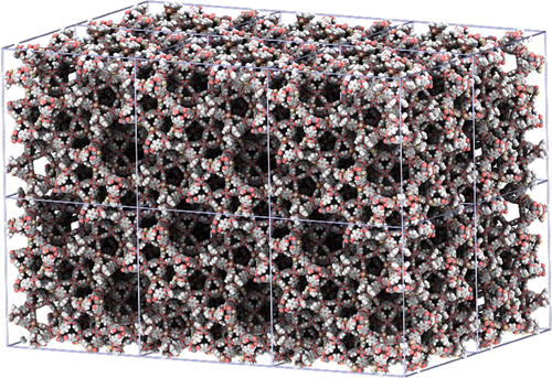
The primitive cell is the smallest repeating unit of a crystalline material. However, the efficiency of perceiving the structure depends on the space scale. Building blocks are easiest shown at the smallest scale, while the overall structure becomes apparent on larger scales. In iRASPA, larger structures can be created by increasing the number of cell replicas. For example, Figure 5 shows a super-cell of unit cells of MIL-101 [43]. Each MIL-101 unitcell (89 Å89 Å89 Å) contains 14416 atoms. The ambient occlusion depends on all replicas, and hence has to be recomputed for every change of number of replicas. The overall picture shows a more clear representation of the distribution of the large cavities of size 32-33 Å.

Figure 5. (Colour online) A super-cell of unit cells of MIL-101; each MIL-101 (89 Å89 Å89 Å) contains 14416 atoms. The ambient occlusion has to be computed based on the super-cell because the outside cells receive more light than the interior cells.

2.7. Collages of structures

Scenes can be a combination of movies of the different components of a system (for example: the cations, anions and the water-solvent as three separate components), or they can be completely unrelated and placed at any position relative to each other. The latter can be used to make ‘collages’. The origin of each movie (or frame) in world-coordinates is set in Cell > Boundingbox-properties. Figure 6 shows an example of placing IRMOF-1,-10 and -16 in one scene, so that their relative sizes become apparent.

2.8. Picture and movie creation

Making great pictures and movies really helps to enhance scientific content of presentations, teaching and publications. Pictures can be made up to the resolution that the video-card supports, in 8- or 16-bits RGB or CYMK TIFF format. By default, the background colour is white, because this is most suitable for journal and book publications. Background options include uniform colours, linear or radial gradients, and images. Figure 7 shows an example of a gradient background and the details of the picture/movie-options.

2.9. Collaboration on a shared document

On macOS High Sierra (10.13), for documents that are stored on ‘iCloud Drive’, you can invite others to your iRASPA document and work on them together in real time. When you invite people to collaborate on a document, the app creates an iCloud.com link for you to send to them via e.g. email or messages. Edits that you and others make to the document appear in real time. You can open a shared document only when your device is connected to the Internet. By default, people that you invite can edit your document. You can change share options and limit who can access it.

If you want to send a copy of a structure, you can send it without collaborating via the ‘share-button’ (top-right) in the toolbar. Structure received via mail can be opened directly using double-clicking, or can be dragged from mail to the iRASPA project-pane.

Figure 6. (Colour online) Three structures, IRMOF-1, IRMOF-10, and IRMOF-16, placed at different positions relative to eachother. The unit cells increase in size as 25.832 Å, 34.2807 Å, and 42.9806 Å, respectively.

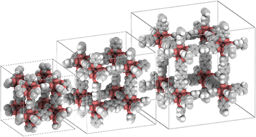
Figure 7. (Colour online) Example of a radial gradient as background. Alternatively, you can use a solid color, a linear gradient or a picture from file as background.

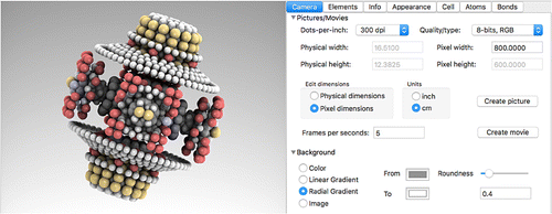
Figure 8. (Colour online) Screening the CoRE MOF and IZA database. All structures in the subtree under the selected directory in the left (project) pane can be queried (for ‘iCloud Public’ approximately 8000 structures). In the right panel the predicate can be edited, the results of the search are shown real-time in the central panel. Here, six structures satisfy the query for structure with a helium void fraction 0.9, geometric nitrogen surface area 5000 m/g, and restricting pore diameter 10.0 Å.

2.10. Public sharing data in the cloud

Public sharing of structures is available via the ’ICLOUD PUBLIC’ section in the project-view panel. The free Cloudkit storage that Apple offers is up to 1PB. The amount of public free storage and data transfer allocated will grow with every new active user with very high limits, for storage 250MB and 2.5 MB per user for the database (up to 10 TB), 10GB assets plus 250MB per user (up to 1PB), and for asset data transfer 2GB plus 50MB per user per month (up to 200 TB per month). The local projects in iRASPA are compressed using an Apple-specific encoder. This algorithm, called LZFSE, is faster than zlib and generally compresses better. Cloud projects are compressed using the Lempel–Ziv–Markov chain algorithm (LZMA) algorithm for high compression ratios.

Cloud-structures can be viewed, but not edited to save band-width. To play around, edit and/or modify the structure, drag them into the local projects first. Figure 8 shows the UI when a directory is selected in the project-view. The right detail-view is a predicate editor allowing the user to create arbitrary complex queries on the cloud-data. The middle content-view show a collection view of all structures satisfying the query. Double-clicking opens the structure for viewing.

Figure 9. (Colour online) The HEXVEM structure (a) from the CoRE MOF database, (b) the conventional cell with spacegroup -F 2 2 3 (spacegroup number 203). The primitive is four times smaller in volume than the conventional cell.

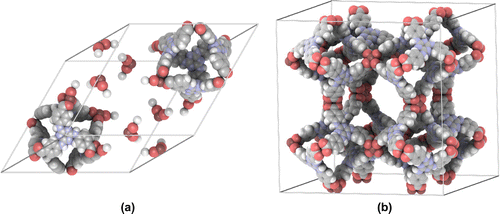
Figure 10. (Colour online) Atoms, bonds, cell boundaries: (a) zoom in showing the (near-)pixel-perfect, anti-aliased, HDR rendering of atoms and bonds, (b) the cut of bonds that cross the unitcell boundary.

2.11. Symmetry operations

Crystallography is the science of finding the symmetry and positions of atoms in crystalline solids [44–48]. Any lattice can be defined on the basis of a cell with the smallest possible volume called a ‘primitive cell’, but many primitive cells are possible. Niggli defined what was termed a ‘reduced cell’ which turned out to be a unique cell [49–52]. Santoro developed an algorithm to find the reduced cell starting from any cell of the lattice [53]. By classifying all materials using the reduced cell, one obtains the basis for a powerful method for compound identification. The reverse, i.e. finding the primitive cell e.g. from the conventional cell, is very useful in quantum mechanical computations to reduce the amount of atoms. iRASPA can perform various symmetry finding operations on crystals, for example automatic spacegroup determination of atomic structures and finding the primitive cell (see Figure 9).

2.12. Atoms, bonds and cell boundaries

In molecular visualisation, usually atoms are drawn as spheres and bonds as cylinders (ball-and-stick model). Ball-and-Stick is the most fundamental and common representation. Atoms are coloured according to their type. Alternatively, the space-filling or VDW representation, renders the atoms with spheres whose radius is the van der Waals atom radius. Here, the representation gives an idea of the molecular external surface and volume. Figure 10 shows iRASPA’s High Dynamics Range (HDR) rendering of atoms and bonds and the treatment of ‘external’-bonds (bonds that cross periodic boundaries).

2.13. Property computation: void-fractions and surface areas

Surface area is the most basic property of porous materials. Along with pore volume, surface area has become the main benchmark characterisation method for any porous material. The most common experimental method for obtaining surface areas involves measuring nitrogen gas adsorption isotherm on the material at 77 K. The isotherm data are then fit by the Brunauer–Emmett–Teller (BET) model, and the surface area is then backed out of the BET parameters. A geometric accessible surface areas can be calculated using a simple Monte Carlo integration technique in which a nitrogen probe (3.681 Å) molecule is rolled along the surface of the framework [54–56]. Walton and Snurr [57] found good agreement for MOFs of the geometric calculation with the BET model, if the appropriate operating range is used for the BET modelling. For small pore systems, e.g. smaller than about 12–13 Å, BET values are questionable because monolayer–multilayer formation and pore filling cannot be distinguished [58]. iRASPA computes an extension of the geometric surface area, i.e. the area of the adsorption surface based on the VDW parameters for the framework and nitrogen as the probe molecule. By computing it on the GPU, the computation can be performed in a matter of seconds.

Figure 11. (Colour online) Pore-volume of MFI-type zeolite: (a) MFI structure with pore adsorption surface, (b) probability density P(d) as a function of the probe-diameter d for MFI with positions taken from IZA; the derivative of this function is the Pore Size Distribution (PSD). The framework model is taken from TraPPE-zeo [59], and we have used and the minimum of the LJ-potential as the upper- and lower-boundary, respectively, of the size of an atom and plot the area in between these as a range of reasonable values. The value computed using the helium void fraction is 0.265 with of helium as 2.64 Å and this value is consistent with the probability density P(d) at this probe diameter. Computed properties are, density 1838.0 kg/m, helium void fraction 0.265, gravimetric surface area 657 m/g, 1209 m/cm, specific volume 0.544 cm/g, accessible pore volume 0.144 cm/g.

iRASPA can also compute helium void fraction within seconds on the GPU. Talu and Myers [60] proposed a simulation methodology that mimics the experimental procedure. For consistency with experiment, the helium void fraction is determined by probing the framework with a nonadsorbing helium molecule using the Widom particle insertion method:(1)

The available pore volume is simply , i.e. the fraction of the total volume V of the cell that is empty. The pore volume is usually normalised as units cm/g (as empty volume per gram of framework). A reference temperature of 25-pagination (298 K) is chosen for the determination of the helium void volume. Figure 11 lists the computed properties for MFI-type zeolite and shows (a) the structure of MFI-type zeolite and the pore system, and (b) the probability density of the diameter of a probe size, i.e. the cumulative pore volume curve algorithm of Gelb and Gubbins [56,61]. The derivative of this function is the Pore Size Distribution (PSD). There is ambiguity in the definition of ‘size’ of an atom; two possible definitions are (1) , the size of the LJ potential at zero energy, (2) , the size of the well-depth of the LJ potential. These two extremes provide a range of reasonable values. The helium void fraction, using K and , produces a very consistent value. The computed values are in general agreement with experimental results for MFI nanocrystals: pore volumes in the range 0.108-0.195 cm/g, and BET surface area in the range 419-785 m/g, depending on the details of the synthesis [62]. Another source gives pore volume 0.14 cm/g and BET surface area 389-467 m/g [63].

The computed helium void fractions compare well to literature values for various zeolites (taken from Abrams and Corbin [64]): RHO 0.465 vs. 0.447, CHA 0.451 vs. 0.407, LTA 0.498 vs. 0.466, ERI 0.411 vs. 0.359, FER 0.332 vs. 0.300, MFI 0.344 vs. 0.265, and FAU 0.522 vs. 0.494 for Abrams and Corbin vs. iRASA helium void fractions, respectively. Abrams and Corbin assume that each group occupies the same volume as in quartz (). Subtracting the volume of the groups from the total volume, and dividing by the total volume yields the void fraction.

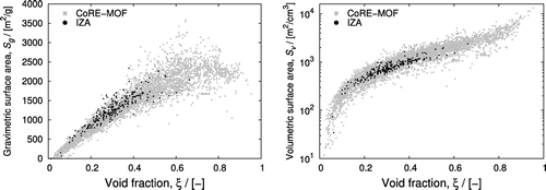
Figure 12. CoRE-MOF and IZA structure property relationships, (left) gravimetric surface area, and (right) volumetric surface area, as a function of helium void fraction.

3. Case studies

3.1. Fast screening

Each year, the synthesis of several hundred new structures is reported and this has created the urgent need to screen these efficiently. Molecular simulations advanced in both speed and accuracy to allow rapid evaluation of (hypothetical-)structures for storage and/or separation devices[65,66]. Screening poses the question: ‘Assuming certain requirements for an given industrial application, what nanoporous material would be most suitable?’ Some examples of screening are: CO screening, screening for CO capture, selective CO adsorption [67,68], alkanes separation [69,70], xylene separation [71], ethylbezene/styrene separation [72], CO/N separation [73], SO, CO and CO separation [74], and CH/H separation [75]. iRASPA contains a command-line utility to facilitate rapid screening. Figure 12 shows computed property relation-ships: the gravimetric and volumetric surface areas as a function of helium void fraction. The CoRE-MOF data encompasses the IZA data, i.e. the variety in MOF-structures is much greater than zeolites, but there exists many MOFs that have similar properties as zeolites. The zeolites form a small subset, with helium void fractions typically lying in the range 0.15 to 0.45. Figure 8 showed the UI that can be used to narrow and track down the structures that result from database queries. It allows the user to see and visualise the typical atomic structures that correspond to a selected helium void fraction and surface area-range.

Figure 13. (Colour online) Screening performance of the iRASPA command-line utility, (left) time for a single evaluation of the surface area, (right) time for a single evaluation of the helium void fraction, both as a function of the number of atoms in the unit cell. Smaller values are better.

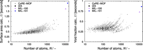
Figure 13 shows the performance of the iRASPA command-line utility. The timing results are performed on a 2009 Mac Pro, 2.4 GHz Intel Xeon using a NVIDIA GeForce GTX 970 videocard. Significant improvements are expected with the new 2017 iMac pro and 2018 Mac pro. The 4764 structures in the CoRE-MOF database can be screened for helium void fractions and surface areas in less than 1.5 h in total, the 233 IZA structures in less than 4 minutes. The vast majority of structures can be screened in less than halve a second per property, and this GPU implementation is typically 1-2 orders of magnitude faster compared to CPU implementations. As a worst case for nanoporous materials, we selected MIL-101 and MIL-100 with, respectively, 14,416 and 11,152 atoms in the unit cell. The computation-time is less than two seconds for the surface-area, and less than a second for the helium void fraction. These numbers can be further improved with more advanced code optimisation.

Figure 14. (Colour online) Cu-BTC with helium energy iso-contour levels: 0 (grey, opacity 0.1), -300 K (plum purple, opacity 0.3), and -410 K (spring green, opacity 1.0): (left) front-view, (right) side-view.

3.2. Examining adsorption sites

Visualization is an important tool to elucidate molecular mechanisms by connecting the macroscopic results (e.g. adsorption isotherms) to the microscopic molecular-level information. Studying the potential energy landscape for a chosen probe molecule allows quick identification of adsorption sites and diffusion path ways. Metal-organic frameworks (MOFs) consist of building blocks that can be easily modified in silico (on the computer). The judicious selection of building blocks allows the pore volume and functionality to be tailored in a rational manner. Because of the design-principle underlying the synthesis, it is important to understand MOF structure–properties relationships.

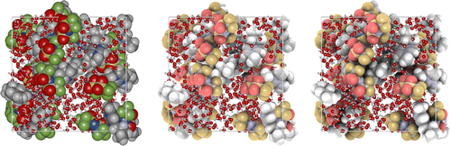
Figure 15. (Colour online) Visualisation of an aqueous solution of ionic liquids: (a) full system, (b) [Tf2N] anion, (c) [C4MIM] cation, (d) water solvent. The computed helium void fraction are 0.141, 0.162 and 0.685, respectively, for the anion, cation and water solvent. The individual contributions add up to 0.988, which is close to unity.

Figure 16. (Colour online) Structure of the liquid at the same geometric void fraction : (left) CO at 230K and (right) methanol at 350K. The chemical potential of CO is -15.9 kJ/mol, and -30.6 kJ/mol for methanol.

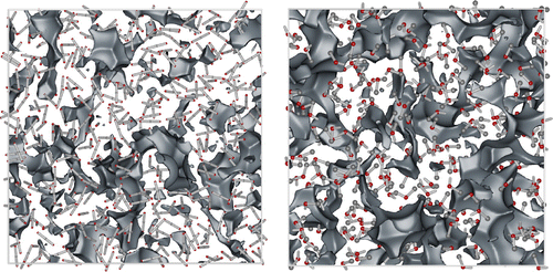
Figure 17. (Colour online) Visualising adsorption: BTEX mixture at 433K in the CoBDP MOF, (top) side view of the channel, (left) front view, (right) front view with adsorbates in stick-style. CoBDP is a rectangular copper-MOF based on a 1,4-benzenedipyrazolate linker: unit cells; unit cell , , , .

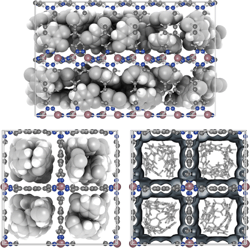
Figure 14 shows the Cu-BTC (also known as HKUST-1) [76], a copper-based benzene-tricarboxylate MOF. The unit cell is cubic with edge-lengths Å, and space group -F 4 2 3. Helium is a good probe molecule to identify possible adsorption sites of small molecules. Any surface location with a high concave curvature is a likely adsorption site while convex surfaces are not. At a concave position, the dispersion interaction with the wall is high. Three surfaces are shown at particular energies (in typical simulation units of Kelvin by converting using Boltzmann’s constant; mulitply by R / 1000 to convert to kJ/mol, where J/K/mol) are shown:

• Energy 0 K, grey colour. This is the most common choice to visualise the pore ‘walls’. The visualised wall reveals the pore connectivity of the system. The channel system is now apparent and any bottle necks for diffusion are easy to identify. Note that, in general, it also immediately reveals ‘pockets’ that are not accessible from the main channel systems. These should be removed and blocked during the simulations. In Cu-BTC, we find small side pockets that are accessible (for small molecules) from the main channel.

• Energy -300 K, plum purple colour. A progressively lower energy surface zooms in on the adsorption sites and diffusion path-ways. The purple surface at -300K shows that small molecules prefer the concave surface parallel to the Cu–Cu dimer and the small side-pockets. The former disappears when the energy is lowered, so the small side-pockets are the dominant adsorption sites for small adsorbates.

• Energy -410 K, spring green colour. An energy close to the lowest energy visualises the shape, topology and connectivity of the adsorption site within the small side-pockets. The adsorption takes place is small green bands in a threefold symmetry from the perspective of the entrance of the pocket. The four exists of the pockets are directed towards the vertices of a regular tetrahedron. At low energy the adsorption sites form a band that is spread out, indicating a fast diffusion path-way within the small pockets. There are however large bottlenecks in between the small pockets as the adsorbates needs to exit the small pocket, cross the main channel, and re-adsorb at another small pocket.

The energy landscapes are crucial to understand the structure. They reflect the viewpoint of the probe molecule, and the pictures are different for each type of adsorbate. For example, for ethane the adsorption sites in the small pockets, but for ethene the adsorption site is at the copper-site. In a mixture, the molecules are adsorbing at different sites (segregation) which differ strongly in interaction energy and Ideal Adsorption Solution Theory (IAST) therefore fails in this case [77].

3.3. Void fractions of liquids

Figure 15 shows an aqueous solution of ionic liquids (cation-anion-water system). Here, hydrogen-bond reduction is the result of anion-water interactions rather than steric effects caused by long alkyl chains of cations [78]. The density of the components is always the same when the volume is fixed: 328, 163 and 659 kg/m, respectively, for the anion, cation and water solvent. Often one would like to know more about the structure of the fluid and what the effective volume and interaction surface is. The computed helium void fraction are 0.141, 0.162 and 0.685, respectively, for the anion, cation, and water solvent. The individual contributions add up to 0.988, which is close to unity. The interaction surface areas are 2642.4, 2863.2 and 1449.2 m/cm, respectively, for the anion, cation, and water solvent. The helium void fraction and interactions surfaces depend on the structure and packing of the molecules.

We previously used this methodology to study the break-down of the Widom test-particle insert (WTPI) method in water and methanol at low temperature [79]. Consider the geometric void fraction defined as(2)

with the number density, and is the volume of the molecular model. Rahbari et al. found that the WTPI method breaks down when the geometric void fraction of the system drops below approximately 0.50, and is independent of the number of hydrogen bonds and the number density. To compute the volume, each interaction site in the molecule is considered to be a sphere with diameter . Therefore, the volume of a molecule with k interaction sites equals the sum of the volumes of all spheres minus the intersection volume between the spheres(3)

where is the total intersection volume between the spheres. We can then compare CO at 230K and methanol at 350K at the same geometric void fraction . Figure 16 shows that the cavities (probed with helium) in the methanol box are larger and more abundant inside methanol liquid box when compared to CO (12.0% vs. 5.8% void). However, the size of methanol ( Å) is larger than CO ( Å). To analysis how difficult it is to insert a probe molecule one cannot use the cavity size alone. It is more difficult to insert a methanol into liquid methanol at than a CO molecule in to liquid CO at because methanol is a larger molecule and inserted into irregularly shaped cavities. The shape of the cavities is determined by the degree of clustering and details of the packing of the molecules and for example affected by temperature and hydrogen-bonding. The lowest Van der Waals insertion energy of the helium probe in the CO liquid is 410 K, while for a helium probe in liquid methanol the lowest insertion energy is 300 K.

3.4. Adsorption

Adsorption is usually described through isotherms, i.e. the amount of adsorbate on the adsorbent at constant temperature as a function of pressure or fugacity. Visualisation can help understand the microscopic origin of adsorption and separation phenomena. In particular, at low pressure the adsorption is dominated by the affinity of the adsorbates with the framework, while at high loadings the adsorption is dominated by entropy. Figure 17 shows a snapshot from a MC-simulation of a 6-component BTEX mixture (ortho-, meta-, and para-xylene, together with benzene, toluene, and ethylbenzene) in the rectangular Co-BDP MOF [80]. The adsorbates are found at the wall and rarely at the centre of the channel.

The packing is the channel at this high pressure is tight, and the ethylbenzene fits less well since its tail is disturbing the packing. Separation mechanisms that are effective at saturation conditions have (in general) to be entropic in nature (saturation corresponds to the high-pressure part of adsorption isotherms). For molecules that have a bulky size and shape (relative to the framework) it is possible to exploit entropy effects to induce a difference in saturation loading [72,81,82].

Figure 18. (Colour online) Visualising diffusion path-ways: The path of a single CO molecule inside the pores of the IRMOF-1 nanoporous material. The adsorption surface has been drawn with a transparent blue colour. (integration step 0.5 fs, snapshot taken every 200 steps, temperature 298 K).

3.5. Diffusion pathways

In many applications of nanoporous materials, the rate of molecular transport inside the pores plays a key role in the overall process. A membrane or adsorption separation process exploits differences in rates of diffusion and/or adsorbed-phase concentrations to differentiate between the different molecular species and separate them. Diffusion properties of guest molecules in microporous materials can be quite sensitive to small differences between different host materials, and molecular-level modelling has, therefore, come to be a useful tool for gaining a better understanding of diffusion in nanoporous materials.

Figure 18 shows a typical path of a rigid CO molecule inside IRMOF-1. The adsorption surface has been drawn with a transparent blue colour. The molecules tumble and swirl from adsorption site to adsorption site (the adsorption sites in IRMOF-1 for small molecules are the sites near the metal-clusters [83]). Diffusion and adsorption are intimately related: the molecules move while staying adsorbed by ‘crawling along the wall’ [84]. Only very rarely molecules are found in the open centre of the cavity.

4. Availability

iRASPA is available free of charge from the App Store and runs on macOS El Capitan (10.11), Sierra (10.12), and High Sierra (10.13).

Acknowledgements

We thank Randall Q. Snurr for access to the CoRE-MOF Database, and Krista S. Walton, Nick C. Burtch, Ariana Torres-Knoop, and Jurn Heinen for valuable suggestions and comments. This work was sponsored by NWO Exacte Wetenschappen (Physical Sciences) for the use of supercomputer facilities, with financial support from the Nederlandse Organisatie voor Wetenschappelijk Onderzoek (Netherlands Organisation for Scientific Research, NWO). T.J.H.V. would like to thank NWO-CW (Chemical Sciences) for a VICI grant.

Additional information

Funding

This work was sponsored by NWO Exacte Wetenschappen (Physical Sciences) for the use of supercomputer facilities, with financial support from the Nederlandse Organisatie voor Wetenschappelijk Onderzoek (Netherlands Organisation for Scientific Research, NWO). T.J.H.V. acknowledges NWO-CW for a VICI grant.

Notes

No potential conflict of interest was reported by the authors.

Appendix 1

Visualisation and implementation details

Primitives

Metal and OpenGL/OpenCL are APIs for encoding and queueing render and compute commands to be submitted to the GPU for execution. The scene is specified imperatively and follows from a sequence of drawing commands. Applications render primitives by specifying a primitive type and a sequence of vertices with associated data. The available basic geometrical primitives are points, lines and triangle, and triangle-strips. Triangle strips start with a triangle, but every additional vertex forms another triangle with the previous two vertices. The number of vertices stored in memory is reduced from 3N to , where N is the number of triangles to be drawn. A list of vertices ‘A,B,C,D,E,F’ would be drawn as ABC, CBD, CDE, and EDF triangles. More complex objects such as discs, spheres, cylinder, cones, and surfaces, must be constructed out of the basis primitives.

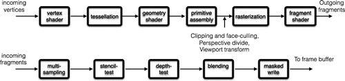
Figure A1. The rendering pipeline is a computer graphics model that describes the conceptual rendering steps of a 3D graphics system from the input vertices to pixels on the screen.

The render pipeline

The rendering pipeline is a computer graphics model that describes the conceptual rendering steps of a 3D graphics system. A simplified version of the pipeline is depicted in Figure A1. On modern hardware, many parts of this pipeline are programmable using what are called ‘shaders’ [85–87].

• Vertex shader. The vertex shaders handle the processing of individual vertices along with vertex attribute data, e.g. normals and colour. In the vertex shader, the vertices and normals are converted from world-coordinates to clip-coordinates.

• Tesselation shaders (optional). After the vertex shader, an optional tesselation stage can be performed. This stage consists of 3 steps: the tessellation control shader, tesselation, and the tessellation evaluation shader (the first and third are programmable). The shaders can see all vertices of a primitive (a form of primitive assembly happens before the shader executes) and subdivide patches of vertex data into smaller primitives, e.g. to smooth a surface.

• Geometry shaders (optional). Just like the tesselation shaders, the optional geometry shader can treat all the vertices of primitive at once, and produce a new primitive or create additional primitives based on the input.

• Primitive assembly. Primitive assembly combines the clip-space vertices into a sequence of primitives. The primitives are classified into points, lines, and triangles. Once the primitives have been assembled, these primitives are tested if they fall within the view-volume. If they do not pass this test, they are ignored in subsequent steps. This test is called ‘clipping’. Primitives that are partially visible (which means that they cross one of the frustum planes) must be handled specially. Triangle primitives can be culled (i.e. discarded without rendering) based on the triangle’s facing in window space. This allows you to avoid rendering triangles facing away from the viewer.

• Rasterisation. Rasterisation determines a bounding box for the triangle in window coordinates and test every fragment inside it to determine whether it is inside or outside the triangle. A fragment is a set of state that is used to compute the final data for a pixel (or sample if multisampling is enabled) in the output framebuffer. The state for a fragment includes its position in screen-space, the sample coverage if multisampling is enabled, and a list of arbitrary data that was output from the previous vertex or geometry shader. This last set of data is computed by interpolating between the data values in the vertices for the fragment. The style of interpolation is defined by the shader that outputs those values. The default provides perspective-correct values of the interpolants to each instance of the fragment shader.

• Fragment shader. The data for each fragment from the rasterisation stage is processed by a fragment shader. The output from a fragment shader is a list of colours for each of the colour buffers being written to, a depth value, and a stencil value. Fragment shaders are not able to set the stencil data for a fragment, but they do have control over the colour and depth values. Applications of the fragment shader are per-pixel lighting, texture mapping, and ray-casting through a volumetric data set.

The fragment data output from the fragment processor is then passed through a sequence of steps.

• Stencil test. When enabled, the test fails if the stencil value provided by the test does not compare as the user specifies against the stencil value from the underlying sample in the stencil buffer. Note that the stencil value in the framebuffer can still be modified even if the stencil test fails (and even if the depth test fails).

• Depth test. When enabled, the test fails if the fragment’s depth does not compare as the user specifies against the depth value from the underlying sample in the depth buffer. Note: though these are specified to happen after the fragment shader, they can be made to happen before the fragment shader under certain conditions. If they happen before the fragment shader, then any culling of the fragment will also prevent the fragment shader from executing.

• Blending. After this, colour blending happens. For each fragment colour value, there is a specific blending operation between it and the colour already in the framebuffer at that location. Logical operations, performing bitwise operations between the fragment colours and framebuffer colours, may also take place.

• Masking. Lastly, the fragment data is written to the framebuffer. Masking operations allow the user to prevent writes to certain values. Colour, depth, and stencil writes can be masked on and off; individual colour channels can be masked as well.

A framebuffer stores information on each pixel (like colour and depth) and can be used as the destination for rendering (either for display or for offline rendering).

Coordinate systems and the virtual camera

By default, OpenGL and Metal work in a left-handed coordinate system called Normal Device Coordinates (NDC), positive axis points right, positive axis points up, and positive depth is further from the viewer. The z-range differs between OpenGL and Metal: OpenGL uses , while metal uses which has advantages on recent hardware when using floating point z-buffers. Inverting the depth-range allows a right-handed system if desired. This volume is often referred to as the unit cube (although it not really is) or the canonical view volume. By default, objects will appear to have the same size everywhere (called orthographic projection). Everything we intend to draw must be defined in the NDC coordinate system. However, it is much more convenient to specify the objects in some world coordinate system by constructing a (virtual) camera.

Figure A2. Coordinate systems for graphics rendering. The natural coordinate system for the hardware is the Normalised Device Coordinates (NDC) which range from in all 3 axes. The steps before are used to simulate a virtual camera. It transform the model-space to world-space and then applies a projection matrix to get camera coordinates. Points outside the viewing frustum are clipped in clip coordinates, and using perspective divide the clip coordinates are transformed to NDC. The last step scales and translates the NDC in order to fit into the rendering screen viewport.

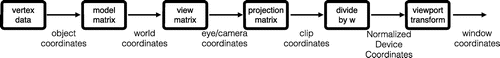
The most common implementation sets the camera fixed at the origin 0, 0, 0 and looks towards the negative z-axis. Changing the view of the camera is performed by actually doing the opposite transformation: the world is translation and rotated. The matrix that performs this operation is called the view matrix which is based on three choices:

(1)	The eye position of the virtual camera (where do you want to pretend your camera is?),
(2)	The location of the centre of the scene (what is your camera looking at?),
(3)	The up-vector of the camera (how are you holding your camera?).

The defaults are: the eye at (0, 0, 0); the centre at and the up is given by the positive direction of the y-axis (0, 1, 0).

A change of basis of one coordinate system to another is mathematically conveniently described by a matrix operation. The three column vectors of the basis must be orthonormal. To create the coordinate system of the camera we can make use of (i) the eye position, (ii) the centre of the scene, and (iii) the up-vector. The first vector we can construct as , i.e. the vector from the eye to where we are looking at. This vector is in the direction of the camera view and normalised. To create the second vector we make use of the up-vector. Note that the up-vector is not orthogonal to the vector , but we can still use the vector and the up vector to create a vector orthonormal to the first vector using . Now that we have two orthonormal vectors and we can recompute the up-vector and force it to be orthonormal . The vector is in the view direction and associated with the z direction and therefore the 3th column; the up-vector u is universally chosen as 0, 1, 0 and associated with the 2nd column (being a y-direction), and the remaining direction forms the 1st column. A rotation matrix can be described as a matrix, but in order to incorporate both rotation and translation mathematically a matrix is required. The matrix operates on vectors of size 4 called ‘homogeneous coordinates’. This vector consists of a x, y, x-triple and a additional dimension called w (for now, ). The view-matrix V transforms world coordinates to camera space and transforms camera coordinates to world coordinates(A1)

The view-matrix works on objects in the scene. But what if the objects themselves can also rotate and have an orientation? Traditionally the ‘world matrix’ is used to move individual models from ‘model space’ to ‘world space’. Then the ‘view matrix’ is used to move all the models from world space into their relative positions in front of the camera (which, in effect, ‘moves the camera’). The view matrix, , multiplies the model matrix and, basically aligns the world (the objects from a scene) to the camera. For a generic vertex, , this is the way we apply the view and model transformations:(A2)

To remap all coordinates contained within a certain bounding box in 3D space into the canonical viewing volume a projection matrix is used. The bounding box, also called the viewing frustum, determines what is contained in you scene and what gets clipped. The projection matrix transforms from camera space to clip space. If part of a triangle sticks out of the frustum then only the part that sticks out is chopped off. Clipping is performed in homogeneous coordinates so that interpolated attributes are calculated correctly. Two different ways of mapping are orthographic and perspective transformations.

Orthographic projection rectangular box is defined by 6 planes: the left- and right-planes, the top-and bottom planes, and the front face, called near-plane) and far-plane. The orthographic projection will not modify the size of the objects no matter where the camera is positioned (useful in CAD, molecular viewers and 2D games). An often used OpenGL matrix definition is:(A3)

For perspective projection, it is more convenient to define the projection matrix through:

(1)	viewing angle or field of view (+fov+)
(2)	aspect ratio
(3)	near and far

where near and far specify the near and far clipping planes. Perspective transformation can be achieved by dividing the vertices by their z-value. If we defined f as(A4)

then the y and z are related by(A5)

At depth z, a y eye coordinate value of y should map on to the viewport coordinate , as it is at the very top of the screen. Similarly, a y eye coordinate value of y should map onto viewport coordinate , and all intermediate y values should map linearly across that range (because perspective projection is linear for all values at the same depth). However, the transformation equation turns out to be non-linear and cannot be represented directly by a matrix. Thus, we invent ‘clip coordinates’ which factor z out of the equations and rather than setting as usual, we set .(A6)

The leads to a right-handed coordinate system before projection and left-handed coordinate system after projection.

We can now redefine the NDC coordinates in terms of the clip coordinates:(A7)

The advantage of separating these two steps is that the first step can now be achieved with a matrix, while the second step is extremely simple. In OpenGL, the projection matrix transforms camera coordinates to clip coordinates (not NDC coordinates). We can rewrite camera-to-clip equations as a matrix (assuming that the w eye coordinate is always 1):(A8)

which is exactly the perspective projection matrix. The projection matrix, , multiplies the product view matrix model matrix and, basically projects the world coordinates to the unit cube (after perspective divide). For a generic vertex, , this is the way we apply the view and model transformations:(A9)

The NDC are scaled and translated to window/screen-coordinates in order to fit into the rendering screen.(A10)

In the fragment-shader we can access an attribute specifier +[[position]]+ in Metal shaders and GLSL variable called +glFragCoord+ for OpenGL, respectively. It contains the window relative coordinate (x, y, z, 1 / w) values for the fragment. The first two values (x, y) contain the pixel’s centre coordinates where the fragment is being rendered. For instance, with a frame buffer resolution of , a fragment being rendered in the bottom-left corner would fall over the pixel position (0.5, 0.5); a fragment rendered into the most top-right corner would have coordinates (799.5, 599.5). For applications that use multi-sampling these values may fall elsewhere on the pixel area.

Depth-buffer

Z-buffering is a way of keeping track of the depth of every pixel on the screen. The depth is an increasing function of the distance between the screen plane and a fragment that has been drawn. That means that the fragments on the sides of the cube further away from the viewer have a higher depth value, whereas fragments closer have a lower depth value. If this depth is stored along with the colour when a fragment is written, fragments drawn later can compare their depth to the existing depth to determine if the new fragment is closer to the viewer than the old fragment. If that is the case, it should be drawn over and otherwise it can simply be discarded. This is known as depth testing.

The value stored in the depth buffer is a value that maps linearly to the near and far plane. In a perspective projection, the z-buffer value is non-linear in camera space. In short, depth values are proportional to the reciprocal of the z value is camera space. There is more precision close to the camera (or eye) and less precision far from the eye. But z values are linear in clip space. Note that the value stored in the depth buffer by default is actually in the range [0, 1], so the depth buffer value is:(A11)

Colour model

In ray-tracing, light is the primitive rendering basis, which leads to photo-realistic images [88]. However, on current hardware ray-tracing, is deemed too expensive for real-time rendering [41], because each pixel can potentially be influenced by all objects in the scene. For real-time rendering like OpenGL and Metal, the most suitable rending primitive is geometry, because each piece of geometry can be handled separately (parallel and independently). The price to pay is that object interaction, like shadows, transparency, and ambient occlusion, must be handled by ad-hoc, special techniques.

The light sources have an effect only when there are surfaces that absorb and reflect light. Each surface is assumed to be composed of a material with various properties. A material might emit its own light (like headlights on an automobile), it might scatter some incoming light in all directions, and it might reflect some portion of the incoming light in a preferential direction like a mirror or other shiny surface.

The OpenGL lighting model considers the lighting to be divided into four independent components: emissive, ambient, diffuse, and specular. All four components are computed independently and then added together:(A12)

In the Phong reflection model the colour is calculated for arbitrary points p on a surface using material properties (Ambient , diffuse , and specular ), light components for each colour (Ambient , diffuse , and specular ) and various vectors as input [89]:(A13)

where l is the vector to the light source, n is the surface normal, v the vector to the viewer, r the reflection of l at p (determined by l and n), and q the distance for surface point p from the light source. These equations are typically modelled separately for R, G and B intensities and different light sources (e.g. directional, point-, and spot-lights) are added. The overall colour is clamped to [0.0,1.0] and then divided into only 256 possible colour values.

The clamping of colours can result in artefacts. Also, if lighting is too dim, the details in the scene are lost. High-dynamic-range (HDR) rendering using floating points buffers allows values greater than 1.0 [19,90] Tone mapping is the process of transforming floating point colour values to the expected [0,1] range, known as Low Dynamic Range (LDR), range without losing too much detail:(A14)

Low ‘exposures’ shows the details in the very bright sections of the screen; high exposures allow you to see details in the dark areas, but washed out the bright parts.

The red, green, and blue (RGB) colour space is common on graphics hardware. However, in printing the CMYK colour space is common. CMYK is a transmissive model, created by subtracting colour components from white [86]. Other used colour models are HLS and HSV. The latter is useful for example to half-desaturate colours [90] like is done in the Qutemole-look [17].

Transparency can be achieved by alpha compositing, i.e. the process of combining an image with a background to create the appearance of partial or full transparency. The interpolation of textures with transparency can be corrected using premultiplied alpha: before interpolation, all RGB colour components are multiplied by that colour’s corresponding alpha value. The blending or compositing of colours is then performed using: .

Billboarding and imposters

Billboards are precomputed 2D textures that always drawn facing the camera. An imposter is defined as anything that replaces actual geometry [91]. This approach renders geometry to an image with a fixed view direction, perspective and shading [92]. Camera-space is very convenient for billboarding because xy-billboards at fixed z automatically face the camera by construction. Any quadric element can be approximated by linear elements called ‘impostors’, quads in the case of spheres and hexahedrons in the case of cylinders and helices (see Figure A3).

For every atom at world coordinate we can get the position in camera-space using:(A15)

In camera space, x and y are left/right and up/down and hence this place always face the camera. We can then easily use this to create a ‘billboard’ of size [-1,+1] and [-1,+1] for the x- and y-axes. Next we scale this square by the size of the atom. However, for perspective view, the actual atom can extend beyond this square so depending on the angle of view this square needs to be made a bit larger.

For orthogonal view, we immediately get the z position from the (x, y) local coordinates as . We can then discard all pixels with and get the sphere shape. Note that we now have not only the position of each visible pixel as (x, y, z) position, but also the normal since we know the location of the centre of the sphere. However, the depth-buffer contains the depth of the billboard, not yet the depth of the sphere [93]. We can explicitly write the depth to the depth-buffer in the fragment shader as(A16)

Note that this makes use of the properties of orthographic projection. For perspective projection, we need to explicitly compute the z-position using ray-intersection of a ray and a sphere: [94]. Ray casting, first coined by Scott Roth in 1982 [95], is a technique for generating an image by casting a ray through each pixel in an image plane, then intersecting these rays with objects in the scene. Once the nearest intersection point has been found, the final pixel colour is determined based on the incoming light and material properties of the object. Instead of performing the ray casting algorithm for each pixel of the screen, we perform it on each billboard. Since we’re in camera space, the camera is at the origin (so the origin can be eliminated from the equations).(A17)

After this procedure, we are in the same situation as when drawing a sphere made up from many, many individual triangles. However, we did it with 2 triangles (making up a square). We can, based on the position and normal, draw the imposter-sphere using for example the Phong reflection model. It looks like a sphere, eventhough it is really drawing a square in a clever way. The vertex-shader is run for these 4 vertices only, the fragment shader for each pixel in the square. One minor downside is that we explicitly have to set the depth-value which on many hardware-type disables ‘early depth’-optimisation (since z-buffer is computed in the fragment shader). Despite this, drawing spheres using imposters is 1 or 2 orders of magnitude faster than drawing it is using many individual triangles or using tesselation shaders. Many imposter algorithms have been developed for spheres, ellipsoids, cylinders, cones, and helixes [17,93,96,99], generic quadratic [100], cubic and quadratic [101], piecewise algebraic surfaces [102], and compound imposters [103]. Note that a small angle of view can lead to large numerical errors [99].

Figure A3. (Colour online) Drawing atoms with imposters: (a) first draw a quad that extends the size of the atom taking perspective projection into account, (b) discard all pixels that are outside a circle the size of the atom, (c) colour each pixel appropriately using the position and normal.

Instanced rendering

Drawing atoms is a typical case suitable for ‘instanced rendering’. The same object is drawn over and over again in different places. Instanced rendering is a method to specify that you want to draw many copies of the same geometry with a single function call. Only the geometry of a single sphere is needed (for sphere-imposters two triangles forming a quad), along with a array of positions for the ‘instances’ of the sphere. For large amount of amounts of atoms, this provides a significant saving of the overhead of many function calls.

In iRASPA also the bonds are treated using instanced rendering of cylinders. However, bonds have an orientations and the cylinders need to be oriented along the distance vectors connecting two atoms. The geometry data is a single cylinder, the instance data is an array of positions for both atoms forming the bond. From the two positions of atoms A and B, the distance vector is computed. Next, we create two additional, perpendicular axes:(A18)

The vectors , , and form a transformation matrix to rotate the single cylinder (aligned in the y-direction) to the bond between atom A and B. Since this is done in the vertex-shader it is very cheap to do.

Picking and selection

3D picking is the process of finding objects of a scene located at a specified point indicated by the mouse. A mouse click on a pixel in the 2D window is matched to the object that is projected to the exact same pixel. The is useful for various interactive uses such as selection, deletion, etc. Picking is implemented by attaching indices to each triangle, object, and structure and use the fragment shader to output the indices at the pixel they belong to. Basically, the ‘color’ buffer is now used not for colours, but only for identifiers of objects. Because no illumination is needed, the picking rendering is cheap (especially when imposters are used), and picking is pixel-perfect by construction. On each mouse click we will read back the identifiers for the clicked pixel. The use of the depth-buffer guarantees we get the index of the top-most object (closest to the camera).

To select atoms in a frustum defined by a rectangular window section (see Figure 2) we need another approach, called ‘unprojecting’. In order to perform the conversion from +glFragCoord+ units to NDC, we must convert +glFragCoord+ values to the range [0, 1] and then compute a simple scale and bias operation to convert them to normalised device coordinates. Depth value in +glFragCoord+ already comes in range [0, 1], but (x, y) values come in screen pixel coordinates, so we need to divide them by the screen size for normalisation. The conversion from window space to NDC-space , clip-space and eye-space is(A19)

where is the projection matrix, the offset of the viewport (usually zero), the width and height of the viewport, and the near and far values passed to +glDepthRange+. To construct the frustum for selection, for each of the four corners of the selection rectangle we convert to world-space twice: once with and once with . The resulting four vectors form the bounding box to search for objects that are contained within.

Figure A4. (Colour online) Illustration showing the mapping of a square texture on a sphere: (a) the folding of the texture around the texture, (d) the front of the sphere, and (g) the result of bi-linear interpolation which shows artefacts where the four corners of the texture patch meet. Tarini et al. solved the continuity problem using periodic boundary conditions on the texture [17]; we now get (b), (e) and (h). Indeed, (h) is continuous, but (e) shows the overall area of the edge is now twice as large. Therefore, a second change is needed: the texture patch is shrunk in texture space by half a texel in every direction [17].

Figure A5. (Colour online) Illustration of ambient occlusion of four spheres: (a) the ambient occlusion texture, (b) ambient occlusion added together with a blue ambient and white specular color, and (c) using texture bi-linear interpolation.

Ambient occlusion using textures

Ambient occlusion (AO) is a technique that approximates the amount of indirect light reaching a point on the surface of an object [104,105]. The amount of light reaching the surface is based on how much light is being occluded by other objects in the world. One of the first applications of ambient occlusion in production rendering was for spatial effects in motion pictures [105]. Unlike local lighting effects where only light coming directly from a light source is taken into account, ambient occlusion is a global method, taking into account other geometry in a scene. It can therefore produce effects otherwise unattainable to standard lighting methods, such as contact shadows. Although it is a very basic approximation to full global illumination, it can be calculated far faster, and is still able to enhance the visual quality of the scene.

For static objects we can precompute the ambient occlusion (because it does not depend on the light direction), leading to fast real-time AO after precomputation. Tarini et al. proposed to stored the pre-computed AO in a global texture [17]. The mapping from texels to x, y, z is [17,106]:(A20)

where . The mapping from x, y, z to texels, up to a normalisation is:(A21)

where . The mapping is gnomonic and hence does not needs its argument to be normalised prior to use. The details of the texture-mapping are shown in Figures A4 and A5.

Figure A6. (Colour online) Storing ambient occlusion in a texture atlas: (a) the IRMOF-1 structure (424 atoms) shown with ambient occlusion, (b) typical depth-texture of a randomly rotated structure showing which pixels receive light (from the camera direction, (c) storage the floating point ambient occlusion in the red-component of a large global texture. Each local texture per atom is pixels, the global texture is of size .

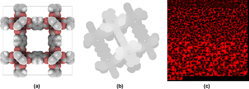
The ambient occlusion for a structure can be stored in an texture atlas, see Figure A6. The IRMOF-1 structure consists of 424 atoms. We can use a texture atlas containing 424 patches of pixels. The maximum texture size that is supported on all macs is , which means that for such a texture atlas for a million atoms we still have a sufficiently large ambient occlusion patch per atom of 1616 pixels. The ambient occlusion is computed by randomly rotating the structure 512 times and accumulating the light per pixel. After normalisation the global texture looks like Figure A6(c).

Glow (bloom) effect

A glow effect is achieved with a post-processing effect called ‘bloom’. iRASPA uses this to differentiate selected atoms from unselected atoms (see Figure A7). First, we render the original image to a temporary buffer. At the same time, we render any glowing parts of the image to a glow buffer. We use an optimised Gaussian filter process on each of the glow textures. To make it fast, we blur in two passes: horizontally to a temporary buffer, and then vertically back to the previous buffer. The temporary buffer and the glow buffer are combined together into the final result. Because the bright regions are extended in both width and height due to the blur filter the bright regions of the scene appear to glow light.

Figure A7. (Colour online) Glow effect: (a) the selected atoms drawn with a glow effect, (b) the selected atoms smeared out using Gaussian blur, (c) the original structure. Adding contribution (b) to (c) leads to figure (a) where the selected atoms appear to ‘glow’.

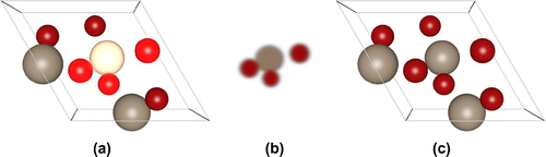
Fast surface extraction

Marching Cubes (MC) is an algorithm for extracting a polygonal mesh of an isosurface from a three-dimensional discrete scalar field [107]. The original method could lead to meshings with holes and was improved upon to construct topologically correct isosurfaces [108]. MC is a completely data parallel algorithm since each cube can be calculated independently on the other cubes and thus ideal for running on GPUs. However, the main problem is that each cube output a different amount of surface triangles (between 0 and 5 triangles). This is a common problem in GPU applications and the solution is often termed ‘Stream Compaction’, which refers to removing unwanted elements from a stream of elements. Smistad et al. solved the compaction problem using a 3D texture version of the Histogram Pyramids (HP) compaction method [109–111]. Suppose the raw data is a texture. The first step is to compute the number of output triangles per texel. Next, the texture is ‘reduced’ using textures halved in size in all dimensions (, , , ). Each substep sums texels into a single value into the next step. Note, the storage per texel is only an 8-bit value for the larger textures (because the maximum output is 5 triangles per texel), up to 16-bits for the smaller textures (for this case). The final texture outputs the total amount of triangles. Importantly, by traversing the HP in Z-pattern, with a criterion described in Refs. [109–111], each possible output index of a surface triangle can be uniquely associated with a 3D texel. So, first the amount of output triangles is computed; next the appropriate GPU memory is allocated to store the triangles, and then for GPU computation proceeded in parallel over all the possible output triangles computing the vertices and normals for the surface triangle based on the raw input data and the constructed HP levels. The 3D texture HP algorithm processes large datasets faster than previous implementations because temporary data is stored in a more efficient format [109].

Capped cylinders

Mac GPUs only support combined depth and stencil formats, the ‘depth32Float_stencil8’ format is supported on all metal devices: A 64-bit combined depth and stencil pixel format with two floating-point components: 32 bits, used for a depth render target, and 8 bits, used for a stencil render target. Stenciling implements a simple state machine in every pixel which can be used to implement capping. Enabling stencil testing adds an additional condition in the fragment pipeline. If stencil testing is enabled, after passing the depth test each fragment will then go through the stencil test. If the fragment passes the stencil test it will be written to the frame buffer, otherwise it will be discarded. The stencil test is very similar to the depth test. In both cases you have a per fragment test used in conjunction with a dedicated buffer. The main difference between the two is the test functions. The stencil buffer can be used to cap clipped solids that intersect with a clipping plane. To draw a cap on a clipped cylinder a three-step process is used [90]: (1) render the front-facing triangles (with clipping enabled) only and clear the stencil to 0, (2) render the back-facing triangles (with clipping enabled) and set the stencil to 1, (3) draw the cap only when the stencil is 1. The stencil buffer is used to track all pixels that make up the interior of the cylinder.

Text

2D overlays of text can be done in Cocoa using CALayers (CATextLayer). This produces high-quality textual overlays. However, 3D annotation has to be done from within Metal/OpenGL (the annotation could be occluded by objects in the scene). Text drawn on billboard using textures are fast, but the text relies on texture interpolation for zooming in and out. A crisp text-boundary cannot be sampled and reconstructed properly using standard texture images (like font-atlases). Recent approaches on high-quality text therefore are based on ‘vector textures’, i.e. 2D surface patterns built from distinct shapes [112].

Signed-distance fields precomputes a representation of a font atlas that stores the glyph outlines implicitly [113]. Specifically, the texel values of a signed-distance field texture correspond to the distance of the texel to the nearest glyph edge, where texels outside the glyph take on negative values. Because the texture data is smoothly varying it will behave nicely under magnification and minification using ordinary bi-linear interpolation. This technique allows quick generation of font atlases which can then be used to draw text on the GPU extremely fast.

Appendix 2

Symmetry and spacegroups

Finding a primitive cell

The fractional positions of all the atoms in a structure are given in some basis B with basis vectors . This might be a P1 structure with all symmetry removed or a supercell with additional translation symmetries and the structure could have been displaced and have an arbitrary rotation. Therefore, we have to first find the full translational symmetry from the translations of the atomic configuration. Hanneman et al. presented the following algorithm for finding the primitive cell [114]:

(1)	Starting from each atom i of the configuration, difference vectors to atoms j () of the same type are calculated. Only those difference vectors whose coordinates relative to the basis B do not exceed 1/2 need to be considered.
(2)	Next, each difference vector is added to the position vectors of the other atoms belonging to the configuration. If all resulting vectors are elements of the set of vectors representing the atoms of the configuration, a translation has been found and it is added to the set T of possible translations (vectors representing the basis B are also included in the set T).
(3)	In the next step, test cells are generated by choosing all possible triplets of vectors from the set T. If such a triplet is linearly independent and the volume of the spanned parallelepiped does not exceed the volume of the simulation cell, the test cell is acceptable, in principle.
(4)	Finally, one of the cells with the smallest volume is chosen as the representative primitive cell.

Note that this choice may result in unconventional cell constants. Therefore, the chosen primitive cell is reduced using the algorithm of Delaunay [115] and the necessary transformation of the chosen primitive cell to its reduced form is performed.

transforming to another basis

Symmetry operations are usually described in the formalism, where is the rotation matrix and is the . A point X(x, y, z) transforms as:(A22)

and a symmetry operation as [45]:(A23)

Find symmetry of the lattice

The next step is to find the rotational symmetry of the reduced Delaunay cell . A brute force algorithm would loop over all possible rotation matrices and check that the metric tensor of the transformed cell is numerically equal to the metric tensor of . The metric tensor , computed from the cell matrix , is given by(A24)

It is sufficient to search for twofold axes to determine the full symmetry. Subjecting the twofolds to group multiplication produces the higher-order symmetry elements, if present [116]. Lebedev et al. introduced the idea of simply enumerating all 3x3 matrices with elements -1,0,1 and determinant one [117]. As an additional requirement group multiplication based on each matrix individually has to produce matrices exclusively with elements -1,0,1. There are only 480 matrices that conform to all requirements. Lebedev et al. argue that this set covers all possible symmetry operations for reduced cells. Only 81 of the 480 selected matrices correspond to twofolds. These are easily detected by establishing which of the matrices produce the identity matrix when multiplied with themselves (and are not the identity matrix to start out with).

Find symmetry of the atomic configuration

Next we find the rotational and translational symmetries for the atomic configuration in the reduced Delaunay cell. The point group of the lattice cannot be lower than the point group of the crystal. Therefore the symmetry of the lattice can be used as a starting point omitting the ones that are not compatible. The resulting symmetry set can be converted to a point group by a count of the number of N-fold symmetries (see Table B1). To find the symmetry operation set of the spacegroup we need to include the translation symmetry into the symmetry elements.

Table B1. Look-up table of the point-group using the number of occurrences of symmetries (, , , , , 1, 2, 3, 4, 6). |N| is the Laue group dependent rotation-part to be used in the construction of a conventional basis.

					Centro-	Enantio-
	(, , , , , 1, 2, 3, 4, 6)	name	holohedry	Laue	symmetric	morphic	|N|
1	(0, 0, 0, 0, 0, 1, 0, 0, 0, 0)	1	Triclinic	1	false	true	0
2	(0, 0, 0, 0, 1, 1, 0, 0, 0, 0)	1	Triclinic	1	true	false	0
3	(0, 0, 0, 0, 0, 1, 1, 0, 0, 0)	2	Monoclinic	2m	false	true	2
4	(0, 0, 0, 1, 0, 1, 0, 0, 0, 0)	m	Monoclinic	2m	false	false	2
5	(0, 0, 0, 1, 1, 1, 1, 0, 0, 0)	2/m	Monoclinic	2m	true	false	2
6	(0, 0, 0, 0, 0, 1, 3, 0, 0, 0)	222	Orthorhombic	mmm	false	true	2
7	(0, 0, 0, 2, 0, 1, 1, 0, 0, 0)	mm2	Orthorhombic	mmm	false	false	2
8	(0, 0, 0, 3, 1, 1, 3, 0, 0, 0)	mmm	Orthorhombic	mmm	true	false	2
9	(0, 0, 0, 0, 0, 1, 1, 0, 2, 0)	4	Tetragonal	4m	false	true	4
10	(0, 2, 0, 0, 0, 1, 1, 0, 0, 0)	4	Tetragonal	4m	false	false	4
11	(0, 2, 0, 1, 1, 1, 1, 0, 2, 0)	4/m	Tetragonal	4m	true	false	4
12	(0, 0, 0, 0, 0, 1, 5, 0, 2, 0)	422	Tetragonal	4mmm	false	true	4
13	(0, 0, 0, 4, 0, 1, 1, 0, 2, 0)	4mm	Tetragonal	4mmm	false	false	4
14	(0, 2, 0, 2, 0, 1, 3, 0, 0, 0)	42m	Tetragonal	4mmm	false	false	4
15	(0, 2, 0, 5, 1, 1, 5, 0, 2, 0)	4/mmm	Tetragonal	4mmm	true	false	4
16	(0, 0, 0, 0, 0, 1, 0, 2, 0, 0)	3	Trigonal	3	false	true	3
17	(0, 0, 2, 0, 1, 1, 0, 2, 0, 0)	3	Trigonal	3	true	false	3
18	(0, 0, 0, 0, 0, 1, 3, 2, 0, 0)	32	Trigonal	3m	false	true	3
19	(0, 0, 0, 3, 0, 1, 0, 2, 0, 0)	3m	Trigonal	3m	false	false	3
20	(0, 0, 2, 3, 1, 1, 3, 2, 0, 0)	3m	Trigonal	3m	true	false	3
21	(0, 0, 0, 0, 0, 1, 1, 2, 0, 2)	6	Hexagonal	6m	false	true	3
22	(2, 0, 0, 1, 0, 1, 0, 2, 0, 0)	6	Hexagonal	6m	false	false	3
23	(2, 0, 2, 1, 1, 1, 1, 2, 0, 2)	6/m	Hexagonal	6m	true	false	3
24	(0, 0, 0, 0, 0, 1, 7, 2, 0, 2)	622	Hexagonal	6mmm	false	true	3
25	(0, 0, 0, 6, 0, 1, 1, 2, 0, 2)	6mm	Hexagonal	6mmm	false	false	3
26	(2, 0, 0, 4, 0, 1, 3, 2, 0, 0)	6m	Hexagonal	6mmm	false	false	3
27	(2, 0, 2, 7, 1, 1, 7, 2, 0, 2)	6/mmm	Hexagonal	6mmm	true	false	3
28	(0, 0, 0, 0, 0, 1, 3, 8, 0, 0)	23	Cubic	m3	false	true	2
29	(0, 0, 8, 3, 1, 1, 3, 8, 0, 0)	m-3	Cubic	m3	true	false	2
30	(0, 0, 0, 0, 0, 1, 9, 8, 6, 0)	432	Cubic	m3m	false	true	4
31	(0, 6, 0, 6, 0, 1, 3, 8, 0, 0)	43m	Cubic	m3m	false	false	4
32	(0, 6, 8, 9, 1, 1, 9, 8, 6, 0)	m-3m	Cubic	m3m	true	false	4

Determine spacegroup from symmetry operations

Any arbitrary set of symmetry operations obtained from the previous steps must belong to one of the 230 spacegroup types, and can be transformed to corresponding standard representation by some change of basis matrix with [118]. The algorithm by Grosse-KunstLeve determines the space group by trying to construct for each of the 230 standard settings. Only one of the trials can succeed. All computations can be performed with symmetry elements alone (no metric is needed). The first step is to find a conventional basis for the atomic configuration. The axes’ direction of Laue-group-specific symmetry operations serve as a new basis. A list of all possible eigenvectors of the rotation matrices serves as a lookup. A rotation axis is the eigenvector with eigenvalue unity. For triclinic, no axes are available and the identity matrix is used. But in general at least one axis direction is available, namely a rotation matrix with the Laue-dependent rotation-part |N| listed in Table B1. Theorem TA4.1 in Boisen en Gibbs (1990) states that a vector is in the plane perpendicular to the axis direction of a proper rotation matrix with rotational order n if and only if where . Hence, to get a list of perpendicular rotation axes, we construct and check for the stored list of all possible axes directions. Once we have 3 axes, we construct a matrix from the 3 vectors and check (if not, we swap two vectors to correct). Next, we determine the shift of the origin, which we attempt for each trial transformation . Here, transforms the set of symmetry operations in the original setting to the set in the primitive setting , and are 6 additional trial loops over transformations for alternative cell choices (needed for monoclinic and orthorhombic space groups). Any space group can be generated from at most 3 generators plus centring operations. For computing the origin, it is sufficient to find and that transforms the generators of the group of symmetry operations of the previous steps to the generators of the group of symmetry operations in one of the 230 standard setting . The resulting equations are(A25)

which can be conveniently solved using the Smith normal form over integers [119–121]. A space group determination typically takes less than a second.

References

- Germann TC, Kadau K. Trillion-atom molecular dynamics becomes a reality. J Mod Phys C. 2008;19(9):1315–1319.
- Dubbeldam D, Calero S, Ellis DE, et al. RASPA: molecular simulation software for adsorption and diffusion in flexible nanoporous materials. Mol Simul. 2016;42(2):81–101.
- Hall SR, Allen FH, Brown ID. The crystallographic information file (CIF) -- a new standard archive file for crystallography. Acta Crystallogr A. 1991;47:655–685.
- Kozlkova B, Krone M, Falk M, et al. Visualization of biomolecular structures: State of the art revisited. Comput Graph Forum. 2017;36(8):178–204.
- Schrödinger LLC. The PyMOL molecular graphics system, version 1.8; 2015 Nov.
- Humphrey W, Dalke A, Schulten K. VMD: visual molecular dynamics. J Mol Graphics. 1996;14(1):33–38.
- Pettersen EF, Goddard TD, Huang CC, et al. UCSF chimera-a visualization system for exploratory research and analysis. J Comput Chem. 2004;25(13):1605–1612.
- Herraez A. Biomolecules in the computer: Jmol to the rescue. Biochem Mol Biol Educ. 2006;34(4):255–261.
- Macrae CF, Edgington PR, McCabe P, et al. Mercury: visualization and analysis of crystal structures. J Appl Crystallogr. 2006;39(3):453–457.
- Sayle RA, Milner-White EJ. RASMOL: biomolecular graphics for all. Trends Biochem Sci. 1995;20(9):374–376.
- Akkermans RLC, Spenley NA, Robertson SH. Monte carlo methods in materials studio. Mol Simulat. 2013;39(14–15):1153–1164.
- Palmer D, Conley M. Crystalmaker; 2007.
- Hanwell MD, Curtis DE, Lonie DC, et al. Avogadro: an advanced semantic chemical editor, visualization, and analysis platform. J Cheminform. 2012;4(1):1–17.
- Momma K, Izumi F. Vesta 3 for three-dimensional visualization of crystal, volumetric and morphology data. J Appl Crystallogr. 2011;44(6):1272–1276.
- Le Muzic M, Autin L, Parulek J, et al. cellVIEW: a tool for illustrative and multi-scale rendering of large biomolecular datasets. In: B\"{u}hler K, Linsen L, John NW, editors. Eurographics workshop on visual computing for biology and medicine; 2015. p. 61–70.
- Grottel S, krone M, Muller C, et al. Megamol-a prototyping framework for particle-based visualization. IEEE Trans Vis Comput Graph. 2015;21(2):201–214.
- Tarini M, Cignoni P, Montani C. Ambient occlusion and edge cueing for enhancing real time molecular visualization. IEEE Trans Visual Comput Graphics. 2006;12:1237–1244.
- Stone JE, Hardy DJ, Ufimtsev IS, et al. Gpu-accelerated molecular modeling coming of age. J Mol Graphics Model. 2010;29(2):116–125.
- Wright RS, Haemel N, Sellers G, et al. OpenGL superbible: comprehensive tutorial and reference. 5th ed. Boston, MA: Addison-Wesley Professional; 2011.
- Movania MM. OpenGL development Cookbook. Birmingham, UK: Packt Publishing; 2013.
- Lo RCH, Lo WCY. OpenGL data visualization Cookbook. Birmingham, UK: Packt Publishing; 2015.
- Scarpino M. OpenCL in action: how to accelerate graphics and computation. Shelter Island (NY): Manning Publications; 2011.
- Munshi A, Gaster BR, Mattson TG, et al. OpenCL programming guide. Boston, MA: Pearson Education Inc; 2012.
- Gaster BR, Howes L, Kaeli DR, et al. Heterogeneous computing with OpenCL. Waltham (MA): Elsevier; 2013.
- Tay R. OpenCL parallel programming development Cookbook. Birmingham, UK: Packt Publishing; 2013.
- Kaeli D, Mistry P, Schaa D, et al. Heterogeneous computing with OpenCL 2.0. Waltham (MA): Elsevier; 2015.
- Buck EM, Yacktman DA. Cocoa design patterns. Boston (MA): Pearson Education Inc; 2010.
- Chisnall D. Cocoa programming developer’s handbook. Ann Arbor (MA): Pearson Education Inc; 2010.
- Hillegass A, Preble A, Chandler N. Cocoa programming for OSX. 5th ed. Indianapolis (IN): Pearson Education Inc.; 2015.
- Anderson F. XCode 6 start to finish: iOS and OS X development. Ann Arbor (MA): Pearson Education Inc.; 2015.
- Mathias M, Gallagher J. Swift programming: the Big Nerd Ranch guide. Indianapolis (IN): Pearson Education; 2016.
- Nahavandipoor V. Concurrent programming in Mac OS X and iOS. Sebastopol (CA): O’Reilly Media Inc.; 2011.
- Chung YG, Camp J, Haranczyk M, et al. Computation-ready, experimental metal-organic frameworks: a tool to enable high-throughput computation of nanoporous crystals. Chem Mater. 2014;26(21):6185–6192.
- Nazarian D, Camp JS, Sholl DS. A comprehensive set of high-quality point charges for simulations of metal-organic frameworks. Chem Mat. 2016;28(3):785–793.
- Baerlocher Ch, McCusker LB, Olson DH. Atlas of zeolite framework types. 6th ed. Amsterdam: Elsevier Science; 2007.
- Callaway J, Cummings M, Deroski B, et al. Protein data bank contents guide: atomic coordinate entry format description. New York (NY): Brookhaven National Laboratory; 1996.
- Kuipers JB. Quaternions and rotation sequences. New Jersey, USA: Princeton University Press; 2002.
- Krone M, Friess F, Scharnowski K, et al. Molecular surface maps. IEEE Trans Visual Comput Graphics. 2017;23(1):701–710.
- Snurr RQ, Bell AT, Theodorou DN. Prediction of adsorption of aromatic-hydrocarbons in silicalite from grand-canonical monte-carlo simulations with biased insertions. J Phys Chem. 1993;97(51):13742–13752.
- Dubbeldam D, Calero S, Maesen TLM, Smit B. Understanding the window effect in zeolite catalysis. Angew Chem Int Ed. 2003;42(31):3624–3626.
- Akenine-Müller T, Haines E, Hoffman N. Real-time rendering. Boca Raton (FL): CRC Press; 2008.
- Easdon R. Ambient occlusion and shadows for molecular graphics [PhD thesis]. Norwich, UK: University of East Anglia; 2013.
- Ferey G, Mellot-Draznieks C, Serre C, Millange F, Dutour J, Surble S, Margiolaki I. A chromium terephthalate-based solid with unusually large pore volumes and surface area. Science. 2005;309:2040–2042.
- Giacovazzo C, Monaco HL, Artioli G, et al. Fundamentals of crystallography. New York (NY): Oxford University Press; 2002.
- Hahn T. International tables for crystallography. In: Volume A: space group symmetry: space group symmetry v.A. IUCr Series. International tables of crystallography. Wiley-Blackwell; Corrected Reprint 2005.
- Rhodes G. Crystallography made crystal clear. Burlington (MA): Elsevier; 2006.
- Rupp B. Biomolecular crystallography: principles, practice and application to structural biology. New York (NY): Taylor and Francis group; 2010.
- Julian MM. Foundations of crystallography with computer applications. Boca Raton (FL): Taylor and Francis group; 2015.
- Niggli P. Krystallographische und strukturtheoretische Grundbegriffe. Vol. 1. Krauchenwies, Germany: Akademische verlagsgesellschaft mbh; 1928.
- Burgers WG. On the process of transition of the cubic-body-centered modification into the hexagonal-close-packed modification of zirconium. Physica. 1934;1(7–12):561–586.
- Krivy I, Gruber B. A unified algorithm for determining the reduced (niggli) cell. Acta Crystallogra Sect A: Crystal Phys Diffr Theor General Crystallogr. 1976;32(2):297–298.
- Grosse-Kunstleve RW, Sauter NK, Adams PD. Numerically stable algorithms for the computation of reduced unit cells. Acta Crystallogr A. 2004;60:1–6.
- Santoro A, Mighell AD. Determination of reduced cells. Acta Crystallogra Sect A: Crystal Phys Diffr Theor General Crystallogr. 1970;26(1):124–127.
- Düren T, Sarkisov L, Yaghi OM, et al. Design of new materials for methane storage. Langmuir. 2004;20:2683–2689.
- Duren T, Millange F, Ferey G, et al. Calculating geometric surface areas as a characterization tool for metal-organic frameworks. J Phys Chem C. 2007;111(42):15350–15356.
- Sarkisov L, Harrison A. Computational structure characterisation tools in application to ordered and disordered porous materials. Mol Phys. 2011;37(15):1248–1257.
- Walton KS, Snurr RQ. Applicability of the bet method for determining surface areas of metal-organic frameworks. J Am Chem Soc. 2007;129:8552–8556.
- de Lange MF, Lin L-C, Gascon J, et al. Assessing the surface area of porous solids: Limitations, probe molecules, and methods. Langmuir. 2016;32(48):12664–12675.
- Bai P, Tsapatsis M, Siepmann JI. TraPPE-zeo: transferable potentials for phase equilibria force field for all-silica zeolites. J Phys Chem C. 2013;117:24375–24387.
- Talu O, Myers AL. Molecular simulation of adsorption: gibbs dividing surface and comparison with experiment. AIChE J. 2001;47:1160–1168.
- Gelb LD, Gubbins KE. Pore size distributions in porous glasses: a computer simulation study. Langmuir. 1999;15:305–308.
- Serrano DP, Aguado J, Morales G, et al. Molecular and meso-and macroscopic properties of hierarchical nanocrystalline zsm-5 zeolite prepared by seed silanization. Chem Mater. 2009;21(4):641–654.
- Wang H, Pinnavaia TJ. Zsm-5 with intracrystal mesopores for catalytic cracking. Stud Surface Sci Catal. 2007;170:1529–1534.
- Probing Intrazeolite Space, Abrams L, Corbin DR. J Incl Phenom Mol Recognit Chem. 1995;21:1–46.
- Wilmer CE, Leaf M, Lee CY, et al. Large-scale screening of hypothetical metal-organic frameworks. Nat Chem. 2012;4(2):83–89.
- Colon YJ, Snurr RQ. High-throughput computational screening of metal-organic frameworks. Chem. Soc. Rev. 2014;43:5735–5749.
- Yazaydin AO, Snurr RQ, Park T-H, et al. Screening of metal-organic frameworks for carbon dioxide capture from flue gas using a combined experimental and modeling approach. J Am Chem Soc. 2009;131(51):18198–18199.
- Bae YS, Snurr RQ. Development and evaluation of porous materials for carbon dioxide separation and capture. Angew Chem Int Ed. 2011;50(49):11586–11596.
- Krishna R, Calero S, Smit B. Investigation of entropy effects during sorption of mixtures of alkanes in MFI zeolite. Chem Eng J. 2002;88(1–3):81–94.
- Dubbeldam D, Krishna R, Calero S, et al. Computer-assisted screening of ordered crystalline nanoporous adsorbents for separation of alkane isomers. Angew Chem Int Ed. 2012;51(47):11867–11871.
- Torres-Knoop A, Krishna R, Dubbeldam D. Separating xylene isomers by commensurate stacking of p-xylene within channels of MAF-X8. Angew Chem Int Ed. 2014;53(30):7774–7778.
- Torres-Knoop A, Heinen J, Krishna R, et al. Entropic separation of styrene/ethylbenzene mixtures by exploitation of subtle differences in molecular configurations in ordered crystalline nanoporous adsorbents. Langmuir. 2015;31(12):3771–3778.
- Haldoupis E, Nair S, Sholl DS. Finding MOFs for highly selective CO2/N2 adsorption using materials screening based on efficient assignment of atomic point charges. J Am Chem Soc. 2012;134(9):4313–4323.
- Matito-Martos I, Martin-Calvo A, Gutiérrez-Sevillano JJ, et al. Zeolite screening for the separation of gas mixtures containing so2, co2 and co. Phys Chem Chem Phys. 2014;16:19884–19893.
- Wu D, Wang C, liu B, et al. Large-scale computational screening of metal-organic frameworks for CH2/H2 separation. AIChE J. 2012;58(7):2078–2084.
- Chui SS-Y, Lo SM-F, Charmant JPH, et al. A chemically functionalizable nanoporous material [Cu3(TMA)2(H2O)3]n. Science. 1999;283(5405):1148–1150.
- Heinen J, Burtch N, Guerra CF, et al. Predicting multicomponent adsorption isotherms in open-metal site materials using force field calculations based on energy decomposed density functional theory. Chem - A Eur J. 2016;22(50):18045–18050.
- Vicent-Luna JM, Dubbeldam D, Gomez-Alvarez P, et al. Microscopic assembly of aqueous solutions of ionic liquids. Chem Phys Chem. 2016;17(3):380–386.
- Rahbari A, Poursaeidesfahani A, Torres-Knoop A, et al. Chemical potentials of water, methanol, carbon dioxide, and hydrogen sulfide at low temperatures using continuous fractional component gibbs ensemble Monte Carlo. Mol Simulat. 2017;44(5):405–414.
- Dinca M, Choi HJ, Long JR. Broadly hysteretic H2 adsorption in the microporous metal-organic framework Co(1,4-benzenedipyrazolate). J Am Chem Soc. 2008;130:7848–7850.
- Torres-Knoop A, Balestra SRG, Krishna R, et al. Entropic separations of mixtures of aromatics by selective face-to-face molecular stacking in one-dimensional channels of metal-organic frameworks and zeolites. Chem Phys Chem. 2015;16(3):532–535.
- Torres-Knoop A, Dubbeldam D. Exploiting large-pore metal-organic frameworks for separations using entropic molecular mechanisms. Chem Phys Chem. 2015;16(10):2046–2067.
- Dubbeldam D, Snurr RQ. Recent developments in the molecular modeling of diffusion in nanoporous materials. Mol Simulat. 2007;33(4–5):305–325.
- Clark LA, Ye GT, Gupta A, et al. Diffusion mechanisms of normal alkanes in faujasite zeolites. J Chem Phys. 1999;111(3):1209–1222.
- Rost RJ, Licea-Kane B. OpenGL shading language. Boston (MA): Pearson Education Inc.; 2010.
- Bailey M, Cunningham S. Graphics shaders: theory and practice. 2nd ed. Boca Raton (FL): Taylor and Francis group; 2012.
- Wolf D. OpenGL 4 shading language Cookbook. Birmingham, UK: Packt Publishing; 2013.
- Pharr M, Jakob W, Humphreys G. Physically based rendering: from theory to implementation. Burlington (MA): Morgan Kaufmann; 2016.
- Phong BT. Illumination for computer-generated images [PhD thesis]. The University of Utah; 1973. AAI7402100.
- McReynolds T, Blythe D. Advanced graphics programming using OpenGL. San Francisco (CA): Elsevier; 2005.
- Maciel PWC, Shirley P. Visual navigation of large environments using textured clusters. Proceedings of the 1995 symposium on Interactive 3D graphics. Monterey, CA, USA: ACM; 1995. p. 95–102.
- Shade J, Lischinski D, Salesin DH, et al. Hierarchical image caching for accelerated walkthroughs of complex environments. Proceedings of the 23rd annual conference on Computer graphics and interactive techniques; New York, USA: ACM; 1996.
- Bajaj C, Djeu P, Siddavanahalli V, et al. Texmol: interactive visual exploration of large flexible multi-component molecular complexes. Visualization, 2004. IEEE; Austin, TX, USA: IEEE; 2004.
- Lengyel E. Mathematics for 3D game programming & computer graphics. Boston (MA): Charles River Media; 2004.
- Roth SD. Ray casting for modeling solids. Computer graphics and image processing. 1982;18(2):109–144.
- Gumhold S. Splatting illuminated ellipsoids with depth correction. In: Proceedings of International Workshop on Vision, Modeling, and Visualization; Munich, Germany; 2003. p. 245–252.
- Sigg C, Weyrich T, Botsch M, et al. GPU-based ray-casting of quadratic surfaces. In: Proceedings of the 3rd Eurographics/IEEE VGTC Conference on Point-Based Graphics, pages 59–65, Aire-la-Ville, Switzerland; Switzerland: Eurographics Association; 2006.
- Bagur PD, Shivashankar N, Natarajan V. Improved quadric surface impostors for large bio-molecular visualization. In: The Eighth Indian Conference on Vision, Graphics and Image Processing, ICVGIP ’12, Mumbai, India, 16--19 December, 2012; 2012. p. 33.
- Falk M, Grottel S, Krone M, et al. Interactive GPU-based visualization of large dynamic particle data. Synthesis Lectures on Visualization. October 2016;4(3):1–121.
- Toledo R, Lévy B. Extending the graphic pipeline with new gpu-accelerated primitives. Technical report. INRIA-ALICE; 2004.
- de Toledo R, Levy B, Paul JC. Iterative methods for visualization of implicit surfaces on GPU. In: Bebis G, Boyle R, Parvin B, Koracin D, Paragios N, Tanveer S-M, Ju T, Liu Z, Coquillart S, Cruz-Neira C, Müller T, Malzbender T, editors. Advances in visual computing. ISVC 2007. Vol. 4841, Lecture notes in computer science. Berlin, Heidelberg: Springer; 2007.
- Loop C, Blinn J. Real-time GPU rendering of piecewise algebraic surfaces. ACM Trans Graphics. 2006;25(3):664–670.
- Grottel S, Reina G, Ertl T. Optimized data transfer for time-dependent, GPU-based glyphs. Proc IEEE Pac Visual Symp. 2009;2009:65–72.
- Zhukov S, Iones A, Kronin G. An ambient light illumination model. In: Drettakis G, Max N, editors. Rendering techniques ’98. Eurographics. Vienna: Springer; 1998. p. 45–55.
- Landis H. Production-ready global illumination. Course notes on Renderman in production. SIGGRAPH 2002; 2002 Jul.
- Praun E, Hoppe H. Spherical parametrization and remeshing. ACM Trans Graphics. 2003;22(3):340–349.
- Lorensen WE, Cline HE. Marching cubes: a high resolution 3D surface construction algorithm. ACM Siggraph Comput Graphics. 1987;21(4):163–169.
- Montani C, Scateni R, Scopigno R. A modified look-up table for implicit disambiguation of marching cubes. Visual Comput. 1994;10(6):353–355.
- Smistad E, Elster AC, Lindseth F. Fast surface extraction and visualization of medical images using opencl and GPUs. The Joint Workshop on High Performance and Distributed Computing for Medical Imaging; 2011.
- Ziegler G, Tevs A, Theobalt C, et al. On-the-fly point clouds through histogram pyramids. 11th International Fall Workshop on Vision, Modeling and Visualization 2006 (VMV2006); 2006. p. 137–144.
- Dyken C, Ziegler G, Theobalt C, et al. High-speed marching cubes using histopyramids. Comput Graphics Forum. 2008;27(8):2028–2039.
- Cozzi P, Riccio C. OpenGL insights. Boca Raton (FL): Taylor and Francis group; 2012.
- Green C. Improved alpha-tested magnification for vector textures and special effects. ACM SIGGRAPH 2007 courses; New York (NY): ACM; 2007. p. 9–18.
- Hannemann A, Hundt R, Schon JC, et al. A new algorithm for space-group determination. J Appl Crystallogr. 1998;31:922–928.
- Delaunay B. Neue darstellung der geometrischen kristallographie. Z Kristallographie-Cryst Mater. 1933;84(1–6):109–149.
- Le Page Y. Computer derivation of the symmetry elements implied in a structure description. J Appl CrystallogR. 1987;20(3):264–269.
- Lebedev AA, Vagin AA, Murshudov GN. Intensity statistics in twinned crystals with examples from the PDB. Acta Crystallogra Sect D: Biol Crystallogr. 2006;62(1):83–95.
- Grosse-Kunstleve RW. Algorithms for deriving crystallographic space-group information. Acta Crystallogr A. 1999;55(2):383–395.
- Storjohann A. Computation of Hermite and Smith normal forms of matrices [PhD thesis]. Waterloo (ON): University of Waterloo; 1994.
- Wan Z. Computing the smith forms of integer matrices and solving related problems [PhD thesis]. Newark, Delaware, USA: University of Delaware; 2005.
- Fontein F. Aspects of computer algebra. Zurich, Switzerland: Spring Semester; 2013.