Towards the simulation of biomolecules: optimisation of peptide-capped glycine using FFLUX

Abstract

The optimisation of a peptide-capped glycine using the novel force field FFLUX is presented. FFLUX is a force field based on the machine-learning method kriging and the topological energy partitioning method called Interacting Quantum Atoms. FFLUX has a completely different architecture to that of traditional force fields, avoiding (harmonic) potentials for bonded, valence and torsion angles. In this study, FFLUX performs an optimisation on a glycine molecule and successfully recovers the target density-functional-theory energy with an error of 0.89 ± 0.03 kJ mol⁻¹. It also recovers the structure of the global minimum with a root-mean-squared deviation of 0.05 Å (excluding hydrogen atoms). We also show that the geometry of the intra-molecular hydrogen bond in glycine is recovered accurately.

Keywords:

• FFLUX
• machine learning
• quantum chemical topology (QCT)
• force field
• peptide
• QTAIM
• kriging

1. Introduction

Many problems in biomolecular modelling, drug design, reactivity and material science can only be tackled by means of force fields for the foreseeable future. In spite of continuing advances in first-principle simulations their time scale and system size remain restricted compared to those handled by force fields. Consequently there remains the challenge of improving force fields such that their predictions are more trustworthy. This challenge is enormous and has been taken up by several groups over the last two decades or more. Disconcerting proofs that the traditional force fields have not yet reached a good degree of predictive power continue to appear. For example, very recent work [1] showed that traditional force fields used in molecular dynamics fail to provide a consistent picture of the complex conformational landscape of intrinsically disordered proteins. Structural information gleaned from ensembles generated by eight all-atom empirical force fields was compared against information from primary small-angle X-ray scattering and NMR. Ensembles obtained with different force fields exhibit marked differences in chain dimensions, hydrogen bonding and secondary structure content. These differences are unexpectedly large: changing the force field was found to have a stronger effect on secondary structure content than changing the entire peptide sequence.

The current abundance of computing power has put into sharper focus the need for accurate force fields. Groups involved in improving traditional force fields admit in the literature that more work needs to be done. A typical recent example is that of Nerenberg et al. [2], who stated that relatively little work has focused on the nonbonded parameters, many of which are two decades old. More troubling was the lack of improvement of amines and phenols even after exhaustive parameterisation of the van der Waals parameters. They blamed this flaw on the more than twenty year old 6-31G*/RESP model but then stated that … a more advanced charge model may yield greater accuracy and also obviate the need for a large number of unique atom types/vdW parameters. More examples [3–6] of such validation work suggest that a strategy of starting afresh in designing a force field architecture is highly desirable and has a better chance of being future-proof if carefully thought through.

This is the strategy we have adopted some time ago, starting with the electrostatic interaction, which urgently needed treatment beyond the traditional point charge [7] paradigm [8]. We introduced high-rank [9] multipolar electrostatics [10], which is the only way to accurately represent the electrostatic interaction at short and medium range [11,12]. However, because of possible divergence of the multipole expansion at very short range [13] atomic multipole moments do not feature in the current article. Instead, for the small system of only 19 atoms studied here, we use exact electrostatics without multipole expansion (although for 1,n (n > 5) interactions it would converge). Note that work is underway that incorporates [14] the electrostatics by multipole expansion, which will guarantee an accurate representation for large systems such as a whole protein. The exact electrostatics used in the current article, both intra-atomic and inter-atomic, are delivered by a quantum chemical topological energy partitioning scheme called Interacting Quantum Atoms (IQA) [15], which was inspired by one of the first calculations of potential energy [16] between topological atoms [17]. These atoms were first proposed [18] by the Bader group leading to the Quantum Theory of Atoms in Molecules (QTAIM) [19]. Both IQA and QTAIM are part of Quantum Chemical Topology (QCT) [20,21], which is a parameter-free partitioning approach, using only the gradient vector.

Polarisation has long been recognised as an important effect that force fields should incorporate in their quest for realism and accuracy. Three popular methods are: (i) polarisable point dipoles [22], (ii) fluctuating atomic charges [23] and (iii) attaching a fictitious negative charge (a Drude particle) [24] to the molecule by a harmonic spring. The first method causes a ‘polarisation catastrophe’, where the dipoles respond in such a way that the interaction energy becomes infinite. This infelicity is typically overcome by damping functions. The point dipole method appears in the potentials [25] of the AMOEBA force field [26], where polarisable point dipoles are located on atomic centres. Within the SIBFA force field, polarisable point dipoles are situated now also at off-nuclear positions [27]. This is analogous to the method in the EFP force field [28,29]. In our force field, however, we use a more powerful and general way to tackle polarisation: machine learning establishes a direct link between an atomic multipole moment and the nuclear positions of surrounding atoms. Initially we used neural networks [30] but a comparison [31] of this machine learning method and a completely different one called kriging [32] ruled in favour of the latter, following our philosophy that prediction accuracy is a priority over training speed. Note that our approach focuses on the result of the polarisation process rather than the process itself, and thus the polarisability. However, it is possible, as was done a long time ago [33], to calculate polarisabilities within the QCT ansatz.

Subsequently, it turned out that the non-electrostatic energy contributions, such as kinetic energy [34], exchange [35] and correlation energies [36] could also be successfully kriged. The IQA approach provides all these energies but they can be grouped (i.e. summed) in various ways. One reason for such grouping can be theoretical: in this paper we use Density Functional Theory (DFT), which forces exchange and correlation to be combined [37]. Also, in this work, we lump all contributions (i.e. kinetic, electrostatic, exchange and correlation) into a single atomic energy denoted . Kriging this well-defined physical quantity equips a topological atom with the knowledge of how to adjust its energy to a previously unseen atomic environment. This approach culminated in the first version of the topological force field called QCTFF, which is described in detail elsewhere [38].

Note that QCTFF completely overhauls the architecture of classical force field such as CHARMM. Indeed, amongst the several fundamental differences are first of all that QCTFF does not categorise interatomic interactions as bonding or non-bonding, thereby avoiding an artificial and debatable boundary [39] between the two. Secondly, QCTFF does not introduce (harmonic) bonding and valence angle potentials, nor torsion potentials, thereby avoiding a proliferation of cross-terms. Furthermore, other ad hoc corrections such as hydrogen bond terms, improper dihedral terms [40] are absent, and certainly the omnipresent E _specific energy term of the ReaxFF [41] force field, which mops up lone pairs, conjugation and other effects. Thirdly, QCTFF ‘sees the electrons’ because it refers to the original reduced first and second order density matrices from which intra-atomic and inter-atomic energies are derived. Moreover, QCTFF handles charge transfer effects (via monopolar polarisation), ideally up to a milli-electron. In summary, QCTFF regards any chemical effect or phenomenon as a result of primary (i.e. physical rather than chemical) energy contributions. With the availability of analytical forces [42], geometry optimisations could be carried out for the first time using this novel architecture, as shown in the case of the water monomer [43].

QCTFF then changed name to FFLUX [44], as it embarks on a much more ambitious journey towards tackling proteins in aqueous solution. On this long journey, the current contribution is a pivotal proof-of-concept showing that FFLUX can successfully geometry-optimise the simplest amino acid in the gas-phase. This amino acid is glycine dipeptide, as it is often referred to in the literature (although it is actually a single amino acid, glycine, capped by N-acetyl and N-methyl groups at the N- and C-termini, respectively, i.e. N-acetylglycyl-N-methylamide). Many details can be found in the first-ever FFLUX geometry optimisation [43] and will therefore not be repeated here.

2. Methodology

2.1. Calculation of atomic energies using IQA

Traditional force fields use essentially penalty functions as functional forms for their energy potentials. In other words, a particular energy such as bond energy, for example, is expressed as an energy change compared to a reference energy that is artificially set to zero, and which corresponds to the bond energy at equilibrium. Such an approach requires a reference coordinate value, which FFLUX does not need. As the value of the coordinate deviates from the reference value, an energy penalty is added in traditional force fields. Such penalty functions are often parameterised harmonic potentials to model bond, angle, improper dihedral and Urey-Bradley energies. Instead, FFLUX regards the atom as the central object (not the bond) and focuses on how the atom’s energy changes. As a result, FFLUX is aware of the huge energies associated with a typical atom, which is of the order of a hundred thousand of kilojoules per mole for a second row atom. IQA quantitatively describes the total energy of an atom, even if the system is not at a stationary point in the potential energy surface. This total atomic energy is comprised of the energy associated with the atom itself (intra-atomic), and with energy resulting from the interaction between the atoms (interatomic). Equation (1(1) ) decomposes the molecular energy, denoted E _IQA ^molec, into atomic energies, one for each atom A, denoted , followed by its breakdown into intra-atomic and interatomic interaction energies,(1)

It is possible to further break down the intra-atomic and inter-atomic energies [35,43] into kinetic, exchange-correlation and electrostatic components, which are not explained because they do not feature in the current work. However, it is important to point out that IQA generates orbital-free quantities, that is, the energies it provides are typically obtained from orbitals but no orbital trace remains once the energies are calculated. This approach simplifies matters, also at the level of forces, thereby avoiding the unnecessary complexity [45] found in orbital-dependent approaches such as EFP. Secondly, FFLUX does not operate within the framework of Rayleigh-Schrödinger perturbation theory [46], which has a large imprint on the architecture of current popular force fields (e.g. CHARMM, AMBER, GROMOS) and even next-generation force fields (e.g. AMOEBA, SIBFA, EFP). More details can be found in Section 2.10 of Ref. [44].

2.2. Kriging and forces

The most explicit account of kriging (also known as Gaussian process regression [47]) in the context of FFLUX can be found in our previous work [48]. As any machine learning method, kriging establishes a mapping between input data (called features) and output data. Kriging operates in a feature space whose dimensionality is equal to that of the number of features (N _feat), using a training set of N _train molecular geometries. FFLUX estimates the molecular energy of a given geometry (previously unseen or seen) as a sum of all the predicted atomic energies, , as shown in Equation (2(2) ),(2)

where μ ^A is the mean value of all the training data points, is the kriging weight of training point j, is the first of two correlation function parameters, which represents the activity of feature-space described by summation index h, is the known feature value from training point j, is the current feature for which a prediction must be made and is the second correlation function parameter, which represents the smoothness of the feature space. Note that in this study is fixed at a value of two and therefore the so-called kernel (i.e. the exponential function) is Gaussian and hence has no cusp, thus assuming a smooth prediction space.

The features used for training and atomic property prediction are defined in the atomic local frame (ALF). Each atom in the system has its own ALF. For sake of completeness we point out that the need for an axis system stems from the installation of multipole moments at an atomic nucleus, and moments are directional. Again, multipole moments do not feature in the current article but have done so in the past when we successfully trained for them. In the future, when both short-range (exact) and long-range (multipolar) electrostatic energies are combined, the ALF will become once again crucial. However, the ALFs have another important role, which applies even to scalar (i.e. non-directional) atomic quantities such as (or the atomic charge). Indeed, an ALF makes it possible to define an atom’s (nuclear) position independently of the global frame and instead only requires the relative positions of other atoms in the system. As a result, an ALF ‘travels’ with its atom, regardless of the global rotation or translation of the molecular system.

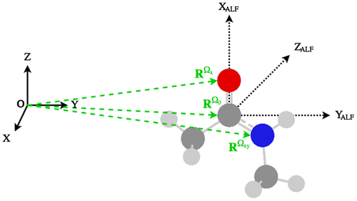
Figure 1 shows the ALF of the carbonyl carbon in N-methylacetamide diagramatically. This carbon or central atom constitutes the origin of the ALF, with Cartesian coordinates , such that , and . Defining the x- and y-axis of the ALF follows the Cahn-Ingold-Prelog convention, in that the heaviest atom neighbouring the central atom defines the ALF x-axis, the second heaviest defines the xy-plane (which in turn defines the ALF y-axis). The z-axis is then defined as orthogonal to both these axes. Subsequently, 3N _atoms – 6 features are defined in the ALF of each atom, giving a total of N _atoms(3N _atoms – 6) features in a molecular system. A complete set of features for a given atom, A, can be seen in Equation (3(3) ),

Figure 1. (Colour online) Schematic illustrating the atomic local frame (ALF) of N-methylacetamide.

(3)

The first three features in Equation (3(3) ) are related to the atoms that define the ALF where is the angle between the x-axis and the y-axis, while the next 3N _atoms – 9 features are the spherical polar coordinates of all remaining atoms. Note that the polar angle θ should not be confused with the activity of feature-space appearing in Equation (2(2) ). The features are defined in Equations (4 (4) )–(9 (9) ), (4) (5) (6)

(7) (8) (9)

where is the position vector of atom n in the ALF of Ω and (i = 1, 2, 3) is a Cartesian coordinate expressed in the ALF. The full account of the above and the derivation of the analytical forces is intricate and given in great detail in previous work by Mills and Popelier [42]. However, note that the definition of χ ^A in Equation (16) of that paper needs to be replaced by Equation (6 (6) ) of the current article. We can only outline some key elements here.

To calculate the force on atom Ω, we take the partial derivative of the predicted energy with respect to global Cartesian coordinates ( α ). By applying the chain rule we can write this force as follows,(10)

Equation (10) gives the force centred on atom Ω in the global Cartesian direction α _i due to the energy and positions of all atoms in the system. Note that the summation over all atoms A includes Ω because as Ω’s position changes will also change because it depends on the position of this atom relative to all others.

The left partial derivative in Equation (10) is simplest to apply as it is not specific to the form of the features f ^A , and is given by Equation (11),(11)

where the ‘sign’ function can adopt a value of −1 or 1. The right partial derivative in Equation (10) has been previously defined for all features by Mills and Popelier [42]. One distinct difference to note is that the Equations (20)–(22) given by Mills and Popelier are replaced in the current work by their preliminary forms in their Supporting Information, such that the partial derivatives of , and are given in Equations (12 (12) )–(14 (14) ), (12) (13) (14)

For completeness we note that the paper by Mills and Popelier used the same convention for global frame Cartesian coordinates and atomic local frame coordinates, i.e. and were confused, and similarly for and . Therefore, in the current paper we defined (see above) the atomic local frame coordinates explicitly using the subscript ALF. Finally, it should also be noted that Equation (19) in the paper by Mills and Popelier the Kronecker-like symbol Δ _Ωn can return a third value other than −1 and 1: if the derivative of the feature has no dependence on the atom Ω then Δ _Ωn returns 0.

2.3. Training

We now discuss the process of training FFLUX, which involves a number of steps as outlined in the recent FFLUX geometry-optimisation work of Zielinski et al. [43] reiterated here:

(1)	Generate conformational ensemble for the construction of both training and (external) test sets.
(2)	Calculate the wavefunction for each conformation.
(3)	Perform IQA calculations to obtain atomic energies.
(4)	Map atomic energies to geometric features using the Kriging machine learning method.
(5)	Perform geometry optimisation using the Kriged atomic energy models.

The computational details associated with each step are outlined below. In this paper, our target molecule is a peptide-capped glycine monomer.

The training data were gathered by distorting about the normal modes evaluated at the global minimum of the peptide-capped glycine [49] obtained at B3LYP/apc-1 level of theory [50] (default GAUSSIAN09 parameters with 6D orbitals and ‘NoSymm’ option). The in-house program EROS was used with a ‘stretch factor’ of 1.1, which means that the normal modes were distorted by a maximum of 10% from the global minimum geometry. For example, a pure single C–C bond (with a length of 1.54 Å) could then take values ranging within the interval 1.39–1.69 Å throughout the data-set. In total, EROS generated 4000 geometries. The wavefunctions for all 4000 conformations were calculated using the B3LYP/apc-1 [50] level of theory in GAUSSIAN09 [51], which is the same level of theory, using the same parameters, as for the global minimum previously found [49]. The IQA energies of the 4000 wavefunctions were calculated using the program AIMAll [52], with the default parameters and AIMAll’s initial implementation for the calculation of the two electron-integrals (as opposed to the more recent so-called ‘TWOe implementation’). AIMAll reproduces the total energy of glycine very well (e.g. −1,198,554.42 kJ mol⁻¹), returning energies that differ only in the second decimal place in kJ mol⁻¹.

We are now in a position to start building kriging models. First, an atomic integration error threshold of L(Ω) = 0.001 a.u. was applied to the 4000 geometries, in order to remove any configurations with a single atomic integration error larger than this threshold. Secondly, 1000 of the remaining conformations were chosen at random and used to build the training set. The in-house program FEREBUS [53] was used to build the Kriging model. As previously mentioned, in this study the values are fixed at 2. Keeping fixed at 2 can be justified from previous work [48] in which the atomic multipole moments in many conformations of histidine dipeptide were predicted. It was found that optimising made very little difference on prediction quality. Fixing to 2 has also been shown to increase computational speed with respect to training by a reduction in the number of parameters required to be optimised [54]. The values of the Kriging parameters are optimised using particle swarm optimisation to maximise the concentrated log-likelihood. Particle Swarm Optimisation as used in FEREBUS has been described fully by Di Pasquale et al. [53].

The trained kriging models can then be used in ‘production mode’, which reduces to a geometry optimisation in this work but will be a finite temperature (condensed matter) molecular dynamics simulation in the near future. The forces calculated using Equation (10) are implemented in an in-house modified version of the molecular dynamics package DL_POLY 4.08 [55]. The FFLUX forces were implemented in a modular fashion to reduce the impact upon the internal working of DL_POLY. OpenMP parallelisation was also implemented over the first sum appearing in Equations (2(2) ) and (11). All 4000 of the initial conformations generated by EROS were used as starting geometries for our geometry optimisations. In addition, to study the behaviour of FFLUX outside of its trained domain we performed a geometry optimisation with a starting geometry of higher energy. This configuration was not one of the 4000 generated by EROS and possessed feature values outside those of the training set domain.

All simulations were run using a 1 fs time step for 5000 fs using the 0 K optimiser. Tests on a variety of systems have indicated that using time steps of less than 1 fs do not result in an increase in accuracy, while time steps greater than 1 fs do results in a decrease in accuracy. The equations of motion were integrated using the velocity Verlet algorithm. The 0 K optimiser uses a minimal temperature (10 K) and resets the particle velocities at each step, which allows the forces on each particle to effectively be only dependent on the current configuration of the system.

3. Results and discussion

3.1. Kriging model quality

The molecular geometries used in the training set were generated by vibrating along the normal modes of the global minimum configuration. A 1000 geometries were then randomly selected to form the training set and 500 were used to build a test set. The quality of the Kriging model can be tested using an S-curve as shown in Figure 2. The prediction error is the absolute difference between the sum of atomic energies, as calculated by AIMAll, and those predicted by the kriging model. The y-axis of an S-curve gives the percentage of the test geometries with an error less than the value read off at the S-curve itself. For example, about 90% of all test geometries (about 450) have an error of (the ubiquitous) 1 kcal mol⁻¹ or ~4 kJ mol⁻¹. Generally, it is desirable that an S-curve has a steep gradient, rapidly reaching for the 100% ceiling. Furthermore, a small mean energy error 2.0 kJ mol⁻¹, (which cannot be read off in Figure 2) and a small maximum error are also hallmarks of quality. Figure 2 shows that all of the test data are predicted with an error <10 kJ mol⁻¹. Moreover, about 40% of the test geometries are predicted with an error of less than 1 kJ mol⁻¹. Given that no design-of-experiment methods have been used to optimise the training set such that the error of prediction is minimised, and that was fixed at 2, the range of prediction error is within reasonable limits.

Figure 2. The prediction error of the sum of the atomic energies for the 500 geometries in the test set.

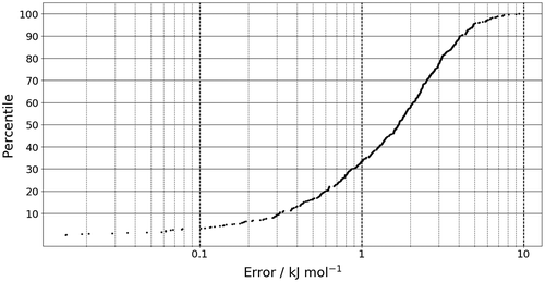
It should also be noted that the energy range of the test set is ~111 kJ mol^-1, making the maximum error of 10 kJ mol⁻¹ an order of magnitude smaller than the range of the energy values. With this in mind, 10 kJ mol⁻¹ is not a large error considering the test set. We can also test for overfitting of the departure model (second term in Equation (2(2) )). An indication that this term would be overfitted is that any predictions are very similar to μ ^A for a given atom. However, we find that our departure model does not suffer from overfitting because no atomistic predictions are closer than 40 kJ mol⁻¹ to their corresponding μ ^A value. Despite the lack of overfitting and the reasonable maximum error, future work will examine further how to improve training sets using methods such as k-fold cross validation or adaptive sampling methods.

3.2. Geometry optimisation

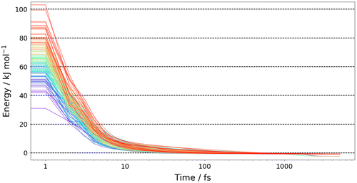
Figure 3 shows the numerically labelled configuration of the target energy minimum, which is the global minimum at B3LYP/apc-1 level of capped glycine. First, we performed geometry optimisations with FFLUX in DL_POLY on all 4000 of the initial geometries generated by EROS. We found that 97% of the energies of the configurations converged to within 1 kJ mol⁻¹ of the target minimum energy. Figure 4 shows the energy convergence over time for a representative 100 starting configurations. There is an initial rapid drop in energy and the majority of geometry optimisations have converged to within 1 kJ mol⁻¹ within 1000 fs. Overall we find that the average root-mean-squared deviation (RMSD) between the final, geometry optimised 4000 configurations and the target minimum is 0.16 ± 0.04 Å (over all 19 atoms per configuration). Overall, the Kriging models are competent at recovering the target minimum’s energy and geometry for conformations within the training domain.

Figure 3. (Colour online) The global minimum geometry of peptide-capped glycine obtained at B3LYP/apc-1 level, with atomic labelling.

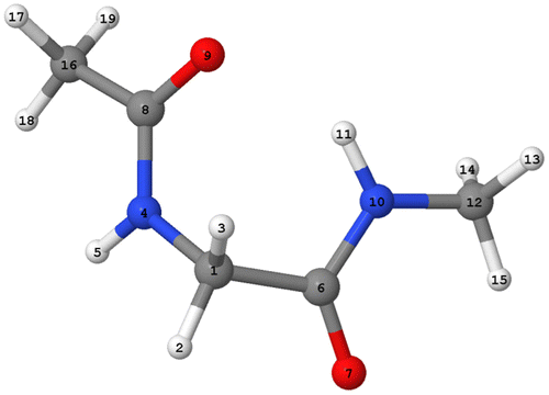
Figure 4. (Colour online) The energy convergence of 100 representative structures from the 4000 randomly generated structures, where the 0 kJ mol⁻¹ values refers to the global minimum energy determined by GAUSSIAN09.

Notes: Colours only serve to separate out the various trajectories.

3.3. Geometry optimisation outside the training domain

Building upon the success of the previous 4000 configurations that were within the training domain, we decided to explore how the Kriging model would behave for a system outside of the training domain. For this geometry optimisation we used an initial configuration that with one its dihedral angles (i.e. φ or C8-N4-C1-C6) set at a value (φ = 180.0^o) far away from the target geometry (φ = −82.3^o). The starting geometry for this test has an RMSD > 0.9 Å compared to the target minimum. We then used FFLUX to optimise this structure at 10 K using the 0 K optimisation method as discussed before. Despite the challenge we have given our Kriging model we find that the optimised geometry is in good agreement with that of the target. Table 1 proves this assertion by comparing a number of geometrical parameters between the exact ab initio values and those predicted by FFLUX. The final energy error of FFLUX compared to the target minimum energy is only −0.89 kJ mol⁻¹ (equivalent to the energy error observed when considering the optimisation of the 4000 configurations within the training space shown in Figure 4, as discussed in Section 3.2), and the RMSD between the optimised and target configurations 0.15 Å (0.05 Å when the hydrogen atoms are excluded). In addition, we are able to predict, with a high degree of accuracy, one of the most important geometric properties of the system: the intra-molecular hydrogen bond. This hydrogen bond is a well-known feature of the so-called C₇ geometry [56] occurring in peptides and proteins, which possesses the 7-membered ring consisting of C₁-C₆-[N₁₀-H₁₁ O₉]-C₈-N₄ where the brackets mark the hydrogen bonded system. The hydrogen bond distance (H…O) predicted by FFLUX has a value of 2.045 Å, which deviates from the exact target B3LYP/acp-1 distance by only 0.001 Å. Meanwhile, the distance between the hydrogen donor (atom N₁₀) and the hydrogen acceptor (atom O₉) is predicted to be 2.940 Å, only 0.004 Å shorter than the distance obtained from the DFT calculation. The hydrogen bond-angle (∠(NHO)) has a value of 145.3°, which has an error of 0.6° compared to the target B3LYP energy. The agreement between FFLUX and DFT is also very good for the φ and ψ dihedral angles, within 5°.

Table 1. A comparison of selected geometric properties of the global energy minimum generated by an ab initio calculation at the B3LYP/acp-1 level of theory and that generated by FFLUX.

Property	Method		Error
	B3LYP	FFLUX
H O/Å	2.046	2.045	0.001
N O/Å	2.944	2.940	0.004
N O/°	145.9	145.3	0.6
ψ/°	67.7	63.3	4.4
φ/°	−82.5	−82.3	0.2
Final energy/kJ mol^−1	−1,198,554.42	−1,198,555.31	−0.89
RMSD/Å			0.15
RMSD (excl. H)/Å			0.05

The large dihedral movement (from φ = 180.0^o to φ = −82.3^o, see above) is shown in an *.avi video uploaded as Supplemental Material. This movie shows the actual [57] topological atoms as they change shape and relative position during the trajectory of the geometry optimisation discussed above. The movie consists of 300 frames taken from this trajectory where the first frame corresponds to an energy 639 kJ mol⁻¹ above the GAUSSIAN09 global minimum while the last frame corresponds to the 447th time step. This end geometry is energetically 0.38 kJ mol⁻¹ higher than the global minimum, given by GAUSSIAN09, and 1.27 kJ mol⁻¹ higher than the final FFLUX minimum. Thus, convergence was not quite reached but the movie was truncated here because little happened, visually, after this frame.

The above results show that, even when given an initial conformation with features far outside the training domain, an optimisation with FFLUX can result in a geometry in good agreement with quantum mechanical calculations, both energetically and geometrically. However, the difference in energy for the initial conformation predicted by FFLUX is far too high compared to that predicated by the DFT calculation, ΔE = ~615 kJ mol⁻¹. This observation is perhaps not that surprising, because when a kriging model is confronted with features outside of its training domain, the second term in Equation (2(2) ) may tend towards zero. Hence, the prediction of an atomic energy atom becomes the constant μ ^A . Because μ ^A is invariant with respect to coordinate change, the atomic forces will tend to zero, which indicates that the model lacks the necessary information to describe this region of feature space. Alternatively, the model may learn incorrect trends, in which case the prediction does not tend towards μ ^A , and the kriging model instead gives large errors on the predicted properties. By considering the atomic energies over the course of the geometry optimisation we are able to distinguish between these two possibilities. In the present case the kriging model does not predict values similar to μ ^A at the initial configuration and instead gives spurious predictions, as shown in Table S1.

We now analyse the convergence of different properties in Figures 5–7. Figure 5 shows the energy of the system (relative to the DFT minimum) as a function of time. The first point to note is that the system tends towards the global minimum despite the large errors in the kriging model’s prediction of the initial conformation. This indicates that the forces derived in FFLUX can have the wrong magnitude outside of the training domain but have the correct direction, that is, towards the minimum for which it was trained. The energy rapidly decreases, such that at 100 fs the energy has dropped from ~650 to ~28 kJ mol⁻¹ (to <5% of the initial energy). From 100 fs onwards the energy converges at a slower rate, such that at 335 fs the energy is within 1 kJ mol⁻¹ of the target minimum. The convergence of the energy is confirmed in Figure 6, which shows the absolute energy difference between the current time step (t _n ) and the previous time step (t _n−1 ). Figure 6 shows that the energy change continually decreases, such that by 1000 fs the energy has converged within 10⁻³ kJ mol⁻¹ (which is less than the integration error associated with AIMAll or 0.004 kJ mol⁻¹ away from the DFT minimum) and by 5000 fs within 10⁻⁶ kJ mol⁻¹. Similarly, Figure S1 shows that the magnitude of forces of each atom decrease to less than 10⁻² kJ mol⁻¹ Å⁻¹ by 5000 fs.

Figure 5. (Colour online) The relative energy (compared to the target minimum) of the system where the initial configuration was outside of the training domain as a function of time.

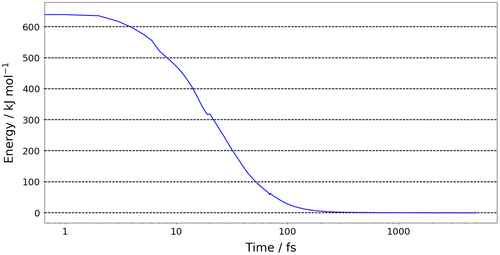
Figure 6. (Colour online) The energy difference of glycine dipeptide, where ΔEnergy (y-axis) is the absolute energy difference of the current time step (t _n ) minus the energy of the previous time step (t _n−1).

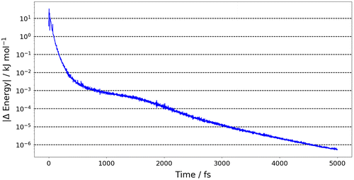
Figure 7. (Colour online) A comparative RMSD of any geometry in the trajectory against the B3LYP target minimum geometry.

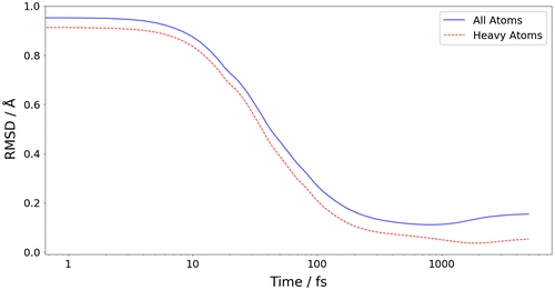
Figure 7 shows the RMSD between the B3LYP/apc-1 global minimum and the conformation at each time step during FFLUX’s geometry optimisation. As seen with the energy convergence in Figures 6 and 7 there is an initial rapid convergence towards the target conformation, with a much smaller rate of change from 1000 fs onwards. When all atoms are included, the RMSD between the final geometry and the target minimum is 0.15 Å but when only the heavy atoms are included, the RMSD drops to 0.05 Å. This difference in RMSD values is due to the hydrogen atoms on the terminal methyl groups being in different positions than those of the target minimum. The reason for the prediction error in methyl hydrogen atoms is the same as discussed earlier regarding the predicted energy error in the initial trajectory configuration (see Table S1), and is due to insufficient sampling for the training set (as seen primarily in Table S2). Therefore, the kriging model currently does not accurately describe these hydrogen atoms. This is not unexpected because the maximum normal mode distortion allowed in the training set was 10%. Therefore, the full rotational barrier of the terminal methyls would not have been properly trained for. Furthermore, harmonic potentials were used to distort the structure by 10%, which also contributed to the poorly sampled dihedral angles. Further investigation regarding training set construction is underway.

Finally, we note that for 5000 time steps the total runtime of FFLUX/DL_POLY was 328 s. Discounting the 25 s time required for initialisation, we calculate the average time per time step as 0.06 s. More importantly, because at 335 fs the optimisation is within 1 kJ mol⁻¹ of the exact energy, only 21 CPU seconds were needed for this degree of optimisation. Note that the 60 ms of CPU time correspond to modest hardware consisting of a single core of a 2.66 GHz Intel Westmere Node. Also note the GNU GFortran compiler was used without compiler optimisations (‘-O0 –g’). Imminent research will focus on optimising the performance of FFLUX/DL_POLY via systematic testing on more recent platforms, with both the implementation of OpenMP and compiler optimisation. Speed-ups of at least a factor 2 are expected.

4. Conclusions

We have shown that the novel force field FFLUX is able to geometry-optimise the peptide-capped amino acid glycine. This case study lends itself to showing further generalisability of the FFLUX code (along with the water optimisation previously mentioned) [43]. Although the study does not show that FFLUX is truly general, we believe that it will succeed for other amino acids, and this case study is a stepping-stone towards oligopeptides. FFLUX recovers the geometry of the heavy atoms to a good accuracy, and achieves this while the global minimum is absent from the training set. FFLUX recovers the global minimum consistently for 97% of the initial geometries within the training domain. For geometries outside of the training domain, FFLUX is unable to accurately predict the atomic energies and forces. However, we find that the direction of the force on the system leads to the system optimising to a region of feature space that is accurately described by the training set, which ultimately results in a geometry in good agreement with the target conformation. In light of this, future work is evidently required to improve the range and accuracy of the training domain, such that FFLUX can be applied to a larger number of conformations.

Disclosure statement

No potential conflict of interest was reported by the authors.

Funding

P.L.A.P acknowledges the EPSRC for funding through the award of an Established Career Fellowship [grant number EP/K005472].

Supplemental data

Supplemental data for this article can be accessed https://doi.org/10.1080/08927022.2018.1431837.

Acknowledgement

We thank F Zielinski for his preliminary work on this research topic, as well as Drs T Fletcher, S Davie, S Cardamone and N Di Pasquale.

References

- Rauscher S , Gapsys V , Gajda MJ , et al . Structural ensembles of intrinsically disordered proteins depend strongly on force field: a comparison to experiment. J Chem Theory Comput. 2015;11:5513–5524.10.1021/acs.jctc.5b00736
- Chapman DE , Steck JK . Nerenberg PS optimizing protein−protein van der waals interactions for the AMBER ff9x/ff12 force field. J Chem Theory Comput. 2014;10:273–281.10.1021/ct400610x
- Mu Y , Kosov DS , Stock G . Conformational dynamics of trialanine in water. 2. Comparison of AMBER, CHARMM, GROMOS, and OPLS force fields to NMR and infrared experiments. J Phys Chem B. 2003;107:5064–5073.10.1021/jp022445a
- Piana S , Donchev AG , Robustelli P , et al . Water dispersion interactions strongly influenec simulated structural properties of disordered protein states. J Phys Chem B. 2015;119:5113–5123.10.1021/jp508971m
- Vitalini F , Mey AS , Noe F , et al . Dynamic properties of force fields. J Chem Phys. 2015;142:084101.10.1063/1.4909549
- Gnanakaran S , Garcia AE . Validation of an all-atom protein force field: from dipeptides to larger peptides. J Phys Chem B. 2003;107:12555–12557.10.1021/jp0359079
- Bultinck P , Vanholme R , Popelier PLA , et al . Geerlings P high-speed calculation of AIM charges through the electronegativity equalization method. J Phys Chem A. 2004;108:10359–10366.10.1021/jp046928 l
- Cornell WD , Cieplak P , Bayly CI , et al . A second generation force field for the simulation of proteins, nucleic acids, and organic molecules. J Am Chem Soc. 1995;117:5179–5197.10.1021/ja00124a002
- Joubert L , Popelier PLA . The prediction of energies and geometries of hydrogen bonded DNA base-pairs via a topological electrostatic potential. Phys Chem Chem Phys. 2002;4:4353–4359.10.1039/b204485d
- Cardamone S , Hughes TJ , Popelier PLA . Multipolar electrostatics. Phys Chem Chem Phys. 2014;16:10367–10387.10.1039/c3cp54829e
- Rafat M , Popelier PLA . A convergent multipole expansion for 1,3 and 1,4 Coulomb interactions. J Chem Phys. 2006;124:144102–144101-144107.
- Popelier PLA , Kosov DS . Atom-atom partitioning of intramolecular and intermolecular Coulomb energy. J Chem Phys. 2001;114:6539–6547.10.1063/1.1356013
- Solano CJF , Pendás AM , Francisco E , et al . Convergence of the multipole expansion for 1,2 Coulomb interactions: the modified multipole shifting algorithm. J Chem Phys. 2010;132:194110.10.1063/1.3430523
- Popelier PLA , Stone AJ . Formulae for the first and second derivatives of anisotropic potentials with respect to geometrical parameters. Mol Phys. 1994;82:411–425.
- Blanco MA , Martín Pendás A , Francisco E . Interacting quantum atoms: a correlated energy decomposition scheme based on the quantum theory of atoms in molecules. J Chem Theory Comput. 2005;1:1096–1109.10.1021/ct0501093
- Popelier PLA . Quantum Chemical Topology. In: Mingos M , editor. The chemical bond – 100 years old and getting stronger. Cham: Springer; 2016. p. 71–117.
- Popelier PLA , Aicken FM . Atomic properties of selected biomolecules: Quantum topological atom types of carbon occuring in natural amino acids and derived molecules. J Am Chem Soc. 2003;125:1284–1292.10.1021/ja0284198
- Bader RFW , Beddall PM . Virial field relationship for molecular charge distributions and the spatial partitioning of molecular properties. J Chem Phys. 1972;56:3320–3329.10.1063/1.1677699
- Bader RFW . Atoms in molecules. A Quantum theory. Oxford: Oxford University Press; 1990.
- Popelier PLA . Quantum chemical topology: on bonds and potentials, structure and bonding. In: Wales DJ , editor. Intermolecular forces and clusters. Heidelberg: Springer; 2005. p. 1–56.
- Popelier PLA . On Quantum chemical topology. In: Chauvin R , Lepetit C , Alikhani E , Silvi B , editors. Challenges and advances in computational chemistry and physics dedicated to ‘applications of topological methods in molecular chemistry’. Cham: Springer; 2016. p. 23–52.
- Stern HA , Rittner F , Berne BJ , et al . Combined fluctuating charge and polarizable dipole models: application to a five-site water potential function. J Chem Phys. 2001;115:2237–2251.10.1063/1.1376165
- Rick SW , Stuart SJ , Berne BJ . Dynamical fluctuating charge force fields: application to liquid water. J Chem Phys. 1994;101:6141–6156.10.1063/1.468398
- Sprik M , Klein ML . A polarizable model for water using distributed charge sites. J Chem Phys. 1988;89:7556–7560.10.1063/1.455722
- Ren P , Ponder JW . Polarizable atomic multipole water model for molecular mechanics simulation. J Phys Chem B. 2003;107:5933.10.1021/jp027815+
- Ponder JW , Wu C , Pande VS , et al . Current status of the AMOEBA polarizable force field. J Phys Chem B. 2010;114:2549–2564.10.1021/jp910674d
- Piquemal J-P , Chelli R , Procacci P , et al . Key role of the polarization anisotropy of water in modeling classical polarizable force fields. J Phys Chem A. 2007;111:8170–8176.10.1021/jp072687 g
- Chen W , Gordon MS . The effective fragment potential model for solvation: internal rotation in formamide. J Chem Phys. 1996;105:11081.10.1063/1.472909
- Gordon MS , Slipchenko L , Li H , et al . The effective fragment potential: a general method for predicting intermolecular interactions. Annu Rep Comput Chem. 2007;3:177–193.10.1016/S1574-1400(07)03010-1
- Darley MG , Handley CM , Popelier PLA . Beyond point charges: dynamic polarization from neural net predicted multipole moments. J Chem Theory Comput. 2008;4:1435–1448.10.1021/ct800166r
- Handley CM , Popelier PLA . A dynamically polarizable water potential based on multipole moments trained by machine learning. J Chem Theory Comput. 2009;5:1474–1489.10.1021/ct800468 h
- Cressie N . Statistics for spatial data. New York (NY): Wiley; 1993.
- In Het Panhuis, M , Popelier, PLA , Munn, RW , et al . Distributed polarizability of the water dimer: charge transfer along the hydrogen bond. J Chem Phys. 2001;114:7951–7961.
- Fletcher TL , Kandathil SM , Popelier PLA . The prediction of atomic kinetic energies from coordinates of surrounding atoms using kriging machine learning. Theor Chem Acc. 2014;133(1499):1491–1410.
- Maxwell P , di Pasquale N , Cardamone S , et al . The prediction of topologically partitioned intra-atomic and inter-atomic energies by the machine learning method kriging. Theoret Chem Acc. 2016;135:L47.10.1007/s00214-016-1951-4
- McDonagh JL , da Silva A , Vincent MA , et al . Machine learning of dynamic electron correlation energies from topological atoms. J Chem Theor Comput. 2018;14:216–224. doi:10.1021/acs.jctc.7b01157.
- Maxwell P , Martín Pendás A , Popelier PLA . Extension of the interacting quantum atoms (IQA) approach to B3LYP level density functional theory. PhysChemChemPhys. 2016;18:20986–21000.
- Popelier PLA QCTFF . On the construction of a novel protein force field. Int J Quant Chem. 2015;115:1005–1011.
- Jensen F . Introduction of computational chemistry. 2nd ed. Chichester: Wiley; 2007.
- Vanommeslaeghe K , Hatcher A , Acharya C , et al . CHARMM general force field: a force field for drug-like molecules compatible with the CHARMM All-Atom Additive Biological Force Fields. J Comp Chem. 2010;31:671–690.
- van Duin ACT , Dasgupta S , Lorant F . Goddard WA ReaxFF: a reactive force field for hydrocarbons. J Phys Chem A. 2001;105:9396–9409.10.1021/jp004368u
- Mills MJL , Popelier PLA . Electrostatic forces: formulae for the first derivatives of a polarisable, anisotropic electrostatic potential energy function based on machine learning. J Chem Theory Comput. 2014;10:3840–3856.10.1021/ct500565 g
- Zielinski F , Maxwell PI , Fletcher TL , et al . Geometry optimization with machine trained topological atoms. Sci Rep. 2017;7:1096.10.1038/s41598-017-12600-3
- Popelier PLA . Molecular simulation by knowledgeable Quantum atoms. Phys Scr. 2016;91:033007.
- Bertoni C , Gordon MS . Analytic gradients for the effective fragment molecular orbital method. J Chem Theory Comput. 2016;12:4743–4767.10.1021/acs.jctc.6b00337
- Stone AJ . Theory of intermolecular forces. 1st ed. Oxford: Clarendon Press; 1996.
- Jones DR , Schonlau M , Welch WJ . Efficient global optimization of expensive black-box functions. J Global Optim. 1998;13:455–492.10.1023/A:1008306431147
- Kandathil SM , Fletcher TL , Yuan Y , et al . Accuracy and tractability of a kriging model of intramolecular polarizable multipolar electrostatics and its application to histidine. J Comput Chem. 2013;34:1850–1861.10.1002/jcc.23333
- Yuan Y , Mills MJL , Popelier PLA , et al . Comprehensive analysis of energy minima of the 20 natural amino acids. J Phys Chem A. 2014;118:7876–7891.10.1021/jp503460 m
- Jensen F . Polarization consistent basis sets. III. The importance of diffuse functions. J Chem Phys. 2002;117:9234–9240.10.1063/1.1515484
- Zupan J , Gasteiger J . Neural networks in chemistry and drug design. 2nd ed. Weinheim: VCH-Wiley; 1999.
- AIMAll, Keith TA . TK Gristmill Software. Overland Park, KS; 2016.
- Di Pasquale N , Bane M , Davie SJ , et al . FEREBUS: highly parallelized engine for kriging training. J Comput Chem. 2016;37:2606–2616.10.1002/jcc.v37.29
- Mills MJL , Popelier PLA . Polarisable multipolar electrostatics from the machine learning method Kriging: an application to alanine. Theoret Chem Acc. 2012;131:1137–123911153.10.1007/s00214-012-1137-7
- Todorov IT , Smith W , Trachenko K , et al . DL_POLY_3: new dimensions in molecular dynamics simulations via massive parallelism. J Mater Chem. 2006;16:1911–1918.10.1039/b517931a
- Popelier PLA , Bader RFW . Effect of twisting a polypeptide on its geometry and electron distribution. J Phys Chem. 1994;98:4473–4481.10.1021/j100067a040
- Rafat M , Devereux M , Popelier PLA . Rendering of quantum topological atoms and bonds. J Mol Graph Model. 2005;24:111–120.10.1016/j.jmgm.2005.05.004