Recent advances in the continuous fractional component Monte Carlo methodology

ABSTRACT

In this paper, we review recent advances in the Continuous Fractional Component Monte Carlo (CFCMC) methodology and present a historic overview of the most important developments that have led to this method. The CFCMC method has gained attention for Monte Carlo simulations of adsorption at high loading, and phase and reaction equilibria of dense systems. It has recently been extended to reactive systems. The main features of the CFCMC method are: (1) Increased molecule exchange efficiency between different phases in single and multicomponent (reactive) systems, which improves the efficiency and accuracy of phase equilibria simulations at high densities; (2) Direct calculation of the chemical potential from a single simulation; (3) Direct calculation of partial molar properties from a single simulation. The developed simulation techniques are incorporated in the open-source molecular simulation software Brick-CFCMC.

KEYWORDS:

• Continuous fractional component Monte Carlo
• expanded ensembles
• chemical potentials
• partial molar properties
• free energy calculations

1. Introduction

Process design in chemical industry requires knowledge of phase equilibria [1,2]. Accurate thermodynamic models are therefore desired for phase equilibria calculations, especially at high pressure [3]. Design of chemical processes at high pressures corresponds to high densities which make more efficient use of the available volume. Examples of such processes are: enhanced oil recovery [4], carbon capture and storage [5], heat-pump cycles [6], the Haber-Bosch process [7], hydrogen compression for transportation and storage [8, 9], etc. [10]. This highlights the importance of performing experiments and modelling of phase equilibria at high pressures to better understand the physics of such processes [11]. However, obtaining accurate phase equilibrium data at high pressures is challenging [11–14]. Performing high-pressure experiments can be hindered due to available technologies, safety, costs, material limitations, etc. [15]. An overview of experimental methods for high-pressure phase equilibria measurements can be found in Refs. [10–14].

In the past decades, advances in computational science have provided possibilities to combine experiments and thermodynamic modelling to develop both descriptive tools and predictive capabilities relevant to processes in the chemical industry [16]. Thermodynamic models used in chemical industry are either fitted to experimental data, empirical, or generic without any fitted interaction parameters [13, 17]. Accurate thermodynamic models are valuable as they can potentially reduce the number of required experimental data points for process design and optimisation [18, 19]. Commonly used thermodynamic models in industry are cubic type Equations of State (EoS) due to low computational costs and simplicity [17, 20–23]. However, it is well-known that cubic type EoS e.g. generic Peng-Robinson (PR) PR EoS [24] or Soave Redlich-Kwong (SRK) EoS [25] often fail to describe phase equilibria of mixtures at high densities or involving polar components [1, 17, 26, 27]. For instance, over 200 different mixing rules for Peng-Robinson EoS were reported for mixtures [18]. This indicates that classical treatment of complex systems is not always sufficient for the analysis and design of chemical processes [28, 29]. The demand for accurate phase equilibria calculations has drawn attention of researchers and industrial partners to more advanced and physically-based methods such as SAFT-type EoS [23, 30–32] and molecular simulation [28, 29]. The advantages of using such models are improved accuracy of phase equilibria calculations and molecular insight into the physics of chemical processes. This molecular insight often complements observations from experiments [28, 29]. In molecular simulation, phase equilibria calculations are mainly performed using the Monte Carlo method, based on the knowledge of the interactions between the molecules in the system [28]. The results from Monte Carlo simulations are stochastic by nature, however, with sufficient sampling, thermodynamically consistent results are expected. The Gibbs Ensemble [33], the grand-canonical ensemble [34, 35], and the osmotic ensemble [28] are most commonly used for phase equilibria calculations using Monte Carlo simulations. The Gibbs ensemble, proposed by Panagiotopoulos in the 80s of the previous century [33, 36] is an efficient way to perform phase equilibria calculations for systems with low or moderate densities, with small finite-size effects (provided that the system is not too close to the critical point) [37, 38]. In this ensemble, two simulation boxes are considered that can exchange energy, volume and molecules, in such a way that the two boxes contain the coexisting phases. To reach chemical equilibrium between the phases, the following conditions are required: equal pressures, equal chemical potentials for each component and equal temperatures. By imposing equal chemical potentials, the number of molecules in each phase is allowed to change. This means having that sufficient molecule exchanges between the phases is essential to have phase equilibrium.

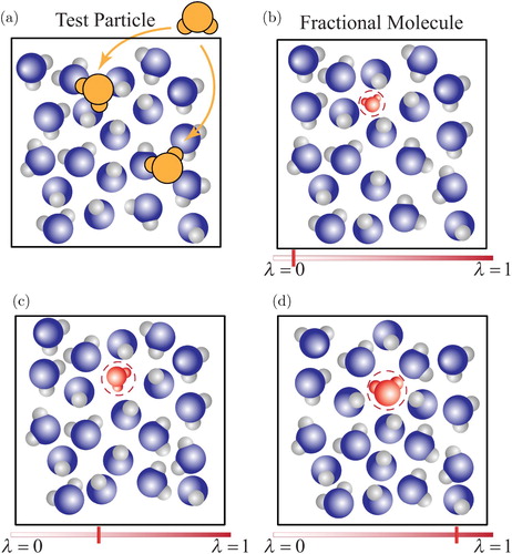
Due to significant advances in computational sciences since the early 1950s [39–41], phase equilibria of complex systems have been investigated ever since [37, 42–44]. For complex systems, it is observed that sufficient exchange of molecules between two phases is hindered due to low probabilities of forming cavities in dense phase. In dense systems, the probability of successful single-step insertions depends on spontaneous formation of cavities large enough to accommodate the molecule. This probability is extremely small if the system density exceeds a certain threshold [45], rendering single-step molecule insertions impractical. Also, deleting a molecule in a single step leaves a cavity in the simulation box with a high energy penalty for the new configuration. Due to very low acceptance probabilities of single-step trial insertions/deletions, such trial moves are not efficient for simulation of dense phases at coexistence. Also, chemical potentials in each phase need to be computed to check whether the condition of chemical equilibrium is met. In sharp contrast to temperature and pressure, the chemical potential (and its derivatives) cannot be determined as a function of atomic positions or momenta of a single configuration [28, 29]. A typical example is the well-known Widom's Test Particle Insertion (WTPI) method [28, 29, 46, 47]. At high densities, the potential energy change due to insertion of the test molecule with the rest of the molecules often becomes very large due to overlaps with other molecules within the system. These overlaps result in large values for the interaction potential leading to a statistical zero Boltzmann factor. In theory, one could perform a very long simulation during which spontaneous cavities would occur once in a while, however this is neither practical nor efficient. In Figure 1(a) single-step molecule insertions are schematically illustrated. It is shown that for a dense system, single-step insertions lead to a large fraction of overlaps. A similar sampling problem of the chemical potential is observed when deleting a molecule from a dense phase [28, 29, 46–50]. The reason is that removing a molecule from a well equilibrated configuration also results in a large energy penalty [45, 50]. Therefore, other Widom-like test molecule insertion/removal methods [46–50] also suffer from similar sampling difficulties. In the past decades, this has led to efforts to develop different methods to overcome the problem of insertion or deletion of molecules and sample the chemical potential. Therefore, specialised simulation techniques are required to both facilitate molecule exchanges between the phases and compute chemical potentials at phase coexistence [51–58]. As single-step insertions are not efficient, it is natural to consider insertions in multiple steps in such a way that the surrounding of a molecule that is inserted can simultaneously adapt. This is the central idea that is applied in expanded-ensembles methods like the recently developed Continuous Fractional Component Monte Carlo (CFCMC) method, by the group of Maginn [59, 60]. In the CFCMC method and expanded ensemble methods in general, interactions of a so-called fractional molecule are scaled with a coupling parameter λ, in such a way that interactions between the fractional molecule and the surrounding ‘whole’ molecules vanish for $\lambda =0$, and that those interactions are fully developed for $\lambda =1$. By including Monte Carlo trial moves for sampling λ, different (expanded) ensembles such as the NPT-, grand-canonical-, reaction-, and Gibbs ensemble can be simulated. The CFCMC method has been used recently to study phase and reaction equilibria of several important systems [42, 61–64]. The expanded ensembles methodology and in particular CFCMC, compete with other methods such as Configurational-Bias Monte Carlo (CBMC) [65, 66], Continuum Configurational Bias (CCB) [67–69], cavity biasing [70] and energy-biasing [71–73]. However, such methods may not be efficient at low temperatures since the performance depends on spontaneous formation of cavities in the system. This sampling problem can be circumvented in expanded ensembles by introducing biasing.

Figure 1. (Colour online) Schematic representation of: (a) test molecule insertions, often resulting in overlaps in dense phases due to the lack of cavities large enough to accommodate test molecules. (b–d) Gradual insertion or removal of a fractional molecule by performing random walks in λ-space. At $\lambda =0$, the fractional molecule does not interact with the other ‘whole’ molecules (ideal gas behaviour) and at $\lambda =1$, the fractional molecule interacts fully with other whole molecules. By performing thermalisation trial moves e.g. translations, rotations, volume moves, etc., the other whole molecules can adapt to the value of λ.

In this paper, we review the recent advancements in CFCMC methodology. Specific applications of the CFCMC method involve different systems in the Gibbs ensemble, reaction ensemble, and isobaric-isothermal ensemble. In Section 2, we briefly review the important developments which have led to the development of the CFCMC method. In Section 3, the application of the CFCMC method in the Gibbs ensemble is discussed. In the Gibbs ensemble, the chemical potential of each phase is directly obtained from a single simulation, by sampling the probability distribution of λ. The condition of chemical equilibrium is met when the chemical potential of both phases are equal. In Section 4, application of the CFCMC method in the reaction ensemble is reviewed. Similar to the Gibbs ensemble, the chemical potentials of reaction products and reactants are obtained by sampling probability distribution of λ. Direct computation of partial molar properties using the CFCMC is described in Section 5. This was used to compute the reaction enthalpy of the ammonia synthesis reaction for pressures up to P=800 bar. In Section 6, the combination of the CFCMC method with other methods such as CBMC and their application to the grand-canonical and osmotic ensembles are reviewed. We have summarised our conclusions in Section 7. The algorithms presented in this manuscript have been incorporated in our open-source molecular simulation software, Brick-CFCMC [62]. The CFCMC algorithms are also implemented in the RASPA software [74, 75].

2. Historical overview of staged insertions and deletions

In this section, an overview of the most important methods leading to advancements in free energy calculations in the framework of expanded ensembles is provided, and a brief summary is shown in Table 1. Here, we highlight several of these methods. In the nineties of the previous century, the idea of expanded ensembles was introduced by Nezbeda and Kolafa [76], Çagin and Pettitt [77, 78] and later reconsidered by Attard [79] and Lyubartsev et al. [51]. In general, an expanded ensemble is a set of sub-ensembles linked by a coupling parameter [53]. This coupling parameter can be a physical parameter (e.g. temperature) or a non-physical parameter (e.g. λ) [80, 81]. In literature, λ is also interchangeably called the scaling parameter or order parameter, however for clarity reasons in the present paper this term is denoted by ‘coupling parameter’. By changing the value of λ in an expanded ensemble (e.g. a CFCMC simulation), one can perform a random walk between the corresponding sub-ensembles and calculate thermodynamic properties such as the chemical potential or partial molar properties. A historical overview of expanded ensemble methods helps to understand the workings and reasons behind the development of CFCMC-type methods. A complete historical overview of simulation methods using expanded ensembles is difficult to find in a single publication. Occasionally, some discrepancies are observed regarding the origin of the method. For instance, in Ref. [82], the expanded ensemble method is attributed to Lyubartsev et al. [51] and in Ref. [83], the first use of the coupling parameter λ is attributed to Escobedo and de Pablo [53]. While Lyubarstev [51] and de Pablo [53, 67] were one of the pioneers of the expanded ensembles, some of the preceding works or ideas leading to their contributions are missing in Refs. [82, 83]. Due to such discrepancies, we make an effort to provide a more comprehensive account of how the expanded ensembles were developed during the past decades. The main ideas fundamental to expanded ensembles can be traced back to the works of Born [84], Onsager [80] and Kirkwood [81], and are thus more than 80 years old. In 1920, Born [84] approximated the free energy of transfer of ions from the gas to the liquid phase as the difference in the energy of charging up a sphere in vacuum and the energy of charging up a sphere in a dielectric medium [77, 85–88]. In fact, Born considered a non-physical (alchemical) pathway for these calculations. In 1933, Onsager showed that for ionic species in a solution, the electrostatic contribution to the chemical potential can be calculated from the non-physical process of charging up the ion in the solution [80]. As stated by Kirkwood [81], this is not restricted to Coulombic charges. In general, fictitious (non-physical) parameters are allowed to be used to manipulate molecular parameters, such as the molecular diameter etc. [81]. For systems of pairwise interactions, the total intermolecular energy $U_N$ of a system containing N molecules is defined as (1) $U_N=\sum _{k<l}{U}_{kl}$(1) where $U_{kl}$ is the pairwise interaction potential between molecules k and l. Within the frameworks of statistical mechanics, it is possible to define a fictitious pair potential using non-physical coupling parameters ${\lambda }_{m\in [1,N]}$ by modifying Equation (1(1) $U_N=\sum _{k<l}{U}_{kl}$(1) ) as follows [81]: (2) $U_N\left({\lambda }_1,{\lambda }_2,\dots {\lambda }_N\right)=\sum _{k<l}{\lambda }_k{\lambda }_l{U}_{kl}$(2) The interaction potential of Equation (1(1) $U_N=\sum _{k<l}{U}_{kl}$(1) ) is recovered if all λ's in Equation (2(2) $U_N\left({\lambda }_1,{\lambda }_2,\dots {\lambda }_N\right)=\sum _{k<l}{\lambda }_k{\lambda }_l{U}_{kl}$(2) ) are set to unity. For a homogeneous fluid, Kirkwood derived an expression for the excess chemical potential using a single coupling parameter for component i [81] (3) ${\mu }_i^{\mathrm{e}\mathrm{x}}={\int }_0^1⟨\frac{\mathrm{\partial }U\left({\lambda }_i\right)}{\mathrm{\partial }{\lambda }_i}⟩\mathrm{d}{\lambda }_i$(3) in which the coupling parameter ${\lambda }_i$ can continuously vary between zero and one. The brackets denote an average in the canonical ensemble. The introduction of λ in the intermolecular interaction potential (as in Equation (2(2) $U_N\left({\lambda }_1,{\lambda }_2,\dots {\lambda }_N\right)=\sum _{k<l}{\lambda }_k{\lambda }_l{U}_{kl}$(2) )) is known as the coupling parameter approach (or charging parameter in electrolyte theory [89]). The coupling parameter approach of Equation (3(3) ${\mu }_i^{\mathrm{e}\mathrm{x}}={\int }_0^1⟨\frac{\mathrm{\partial }U\left({\lambda }_i\right)}{\mathrm{\partial }{\lambda }_i}⟩\mathrm{d}{\lambda }_i$(3) ) is often referred to as thermodynamic integration and is also fundamental to the development of expanded ensembles [28, 52, 57, 76, 87–101]. The coupling parameter approach was used by Squire and Hoover [58] to calculate the free energy of vacancy formation in rare-gas crystals. Helfland et al. [90, 102] used the coupling parameter approach [81] for developing Scaled Particle Theory (SPT). In SPT, the coupling parameter λ is used to scale the distance parameter in the pair potential. The pairwise interaction potential of the ‘fractional’ molecule k with molecule l is a function of $U=U\left(r_{lk}/\lambda \right)$. Free energy calculations using SPT are inspired by the pioneering work of Kirkwood [81].

Table 1. A historical overview of the most important methods and developments leading to advancements in staged insertions and free energy calculations in the framework of expanded ensembles.

Year	Author(s)	Method	Application/examples
1920	Born [84]	Using a non-physical pathway for calculating the free energy of ion transfer from the gas to the liquid phase	Free energy calculations in electrolyte solutions
1933	Onsager [80]	Introduction of alchemical (non-physical) parameters to manipulate the intermolecular interaction potential	Free energy calculations in electrolyte solutions
1935	Kirkwood [81]	Introduction of the coupling parameter method and thermodynamic integration	Computation of the chemical potential in a homogeneous fluid
1955	Rosenbluth and Rosenbluth [40]	Self-avoiding random walk for generating polymer conformations with a certain statistical weight	Three-dimensional random walk of chains up to 64 segments
1960	Helfland et al. [90]	Application of the coupling parameter method in scaled particle theory to scale the intermolecular distance between a particle pair	Rigid spheres, square wells, LJ potential
1963	Widom [46]	Widom's test particle insertion method	Lattice-gas model.
1985	Griffiths et al. [55]	Introduction of the gradual insertion and deletion method for computing the chemical potential	Two-dimensional LJ fluid
1988	Harris and Rice [103]	Computation of chemical potentials of chain molecules by discretizing chain conformations	Amphiphilic chains
1990	Siepmann [104]	Direct simulation of flexible chain molecules; combining Widom's test particle insertion method and self-avoiding random walk	Monolayer systems on a lattice
1991	Nezbeda et al. [76]	Combination of gradual test molecule insertion and Widom's test particle insertion method in the NVT ensemble (semi-grand-canonical ensemble) and the grand-canonincal ensemble	Hard-sphere fluid at high densities
1991	Çagin et al. [77]	Introduction of the concept of fractional molecules in grand-canonical MD, evolution of the coupling parameter follows a deterministic approach	Liquid Argon
1991	Kumar et al. [105]	Introducing the chain increment method. Computation of segmental (incremental) chemical potential for chain molecules by appending/removing segments to/from the ghost molecule	Homopolymers in the subcritical and supercritical regime
1992	Kumar [106]	The Hybrid Real Test Particle Method. The test molecule is allowed to move around in the simulation box before deletion.	LJ systems
1992	Lyubartsev et al. [51]	Method of expanded ensembles, free energy differences for a wide temperature range from a single simulation	Hard-core potential (PRM-electrolyte)
1992	Siepmann and Frenkel [65]	Configurational-Bias Monte Carlo (CBMC)	Single chains on a two-dimensional lattice
1992	Frenkel et al. [66]	Extension of the CBCMC to continuously deformable molecules and computation of the chemical potential	Fully flexible chains of 10 to 20 segments
1992	de Pablo et al. [67]	Continuum Configurational Bias (CCB) ghost-chain method. Growing the test molecule segment by segment	Polymeric systems (limited to short chains)
1993	Attard [79]	Computation of the chemical potential using a force-balance Monte Carlo technique	Hard-sphere fluids
1994	Müller et al. [107]	Free energy calculations using thermodynamic integration for excluded volume interactions.	Lattice polymers up to 80 monomers.
1994	Lyubartsev et al. [108]	Combination of the expanded ensemble method and constant temperature MD simulations, stochastic changes of the coupling parameter during the simulation.	LJ and water systems
1994	Wilding et al. [52]	An efficient implementation of the method by Müller et al. Computing the chemical potential by gradually coupling and decoupling a ghost chain molecule in a single simulation [107][107]	Complex polymers, branched or ring structures
1994	Beutler et al. [109]	Introduction of a new functional form for a stable soft-core for efficient free energy calculations for van der Waals and Coulombic interactions	Polar nitrogen atoms and carbon atoms
1994	Kaminsky [93]	Computation of the thermodynamic properties in augmented ensembles, using an intermediate diameter approach	High density LJ fluid
1995	Lo et al. [110]	Introduction of an alternative Hamiltonian and application of a soft core potential in extended grand-canonical MD simulations	Vapor Liquid equilibrium of the LJ system
1995	Escobedo et al. [54]	Introduction of the Expanded Variable Length Chain (EVALENCH) method, single simulation computations using segmental insertions	Polymers applicable to all chain lengths
1996	Escobedo et al. [111]	Improving the efficiency of the EVALENCH method using the Semianalytical Local Mapping (SEAMAP) method	Single simulation of chemical potentials of long chains at high densities
1996	Escobedo et al. [53]	Expanded grand-canonical and Gibbs ensemble simulation of polymers	Hard-core chain fluids and square-well chains
1998	Meirovitc [112]	A tunable method for computing the chemical potential of chain polymers by combining the chain increment method, the scanning method, and a combination of the Rosenbluth technique and the WTPI method	Systems of chaing lengths 30 and 50
1999	Strnada et al. [115]	Computation of the chemical potential in the extended Gibbs ensemble	Binary mixtures of square-well fluid and hard-spheres
2000	Bunker et al. [116]	Parallel excluded volume tempering for polymer chains using a soft core potential	The off-lattice Kremer-Grest model for polymers for lenghts up to 200 monomers
2001	Vlugt et al. [212]	Application of a soft core potential in the grand-canonical ensemble to couple/decouple attractive and excluded volume interactions	Binary LJ systems
2003	Boinepalli et al. [118]	Hybrid MD-MC grand-canonical simulation, the evolution of the coupling parameter is deterministic.	LJ system
2005	Lísal et al. [119]	Expanded-Ensemble Osmotic Molecular Dynamics (EEOMD) method. The changes in the coupling parameter are stochastic using transition probabilities from the grand-canonical ensemble	NaCl in water at ambient conditions
2007	Shi et al. [59]	Continuous Fractional Monte Carlo (CFCMC) using adaptive biasing method in open ensembles (grand-canonical ensemble)	LJ, water, CO-ethanol binary systems
2008	Shi et al. [60]	Extension of the CFCMC method to the Gibbs ensemble	LJ, water, SO2
2011	Pham et al. [120]	Identifying low variance pathways for free energy calculations	Application for a generalized soft-core potential
2011	Rosch et al. [42]	Application of the CFCMC method in the reaction ensemble	Propene methathesis reaction and methyl-tetr-butyl-ether (MTBE) synthesis
2014	Torres-Knoop et al. [121]	CB/CFCMC hybrid method; combination of the CFCMC method with the CBMC method	Single and five-component isomers of hexane in Fe2(BDP)3
2015	Sikora [122]	Combination of the CBCMC and CFCMC methods based on the approach of Torres-Knoop et al. [121]	High density adsorption in metal-organic frameworks
2016	Poursaeidesfahani el al. [123]	Improving the efficiency of the CFCMC method in the Gibbs ensemble by using a single fractional molecule for direct computation of the chemical potential	LJ and water systems
2017	Poursaeidesfahani el al. [61]	Efficient application of the CFCMC method in the reaction ensemble	LJ system and the ammonia synthesis reaction
2017	Yoo et al. [56]	Discrete Fractional Monte Carlo, a modified version of the CFCMC method using discrete staging is used instead of the continuous change of the coupling parameter	C10E4 and water
2018	Mullen et al. [124]	Identity changes between the reactants and reaction products in combination with the CFCMC method (semi-grand trial move)	CO2 absorption in the reactive ionic liquid triethyl(octyl)phosphonium 2-cyanopyrrolide
2018	Rahbari et al. [125]	Computation of partial molar properties by combining the WTPI method and the CFCMC method	Binary LJ color mixture, ternary mixtures of ammonia, nitrogen and hydrogen
2019	Rahbari et al. [126]	An alternative scheme to directly sample the states λ = 1 and λ = 0 leading to an increased accuracy of computed chemical potentials	SPC/E water and TraPPE methanol, LJ systems
2020	Rahbari et al. [127]	Multiple free energy calculations and computation of partial molar properties by combining the CFCMC method and umbrella sampling [128]	Aqueous methanol mixtures and LJ systems

In the early 1990s, Nezbeda and Kolafa [76] introduced a modified version of WTPI method [46] by combining SPT [90, 129] and multistage sampling [55]. In this method (originally tested for a hard-sphere fluid) [76], the test molecule is inserted in multiple stages. First, test molecule i is inserted as a point, not interacting with the rest of the system. Second, the diameter of the test molecule ${\sigma }_i$ is allowed to fluctuate during the simulation. The values of intermediate ${\sigma }_i$ steps are a priori unknown and need to be guessed for discrete staging [76, 130]. In this expanded ensemble, random walks are performed between the selected values of ${\sigma }_i\in ({\sigma }_1,{\sigma }_k)$ each corresponding to a sub-ensemble (k corresponds to the $k^{\mathrm{t}\mathrm{h}}$ sub-ensemble where the test molecule is maximally coupled). Schematically, one can represent the random walk between the sub-ensembles as [76] (4) $\begin{array}{rl}& \underset{W_0}{\left[N\right]}⟷\underset{W_1}{\left[N+{\sigma }_1\right]}⟷\cdots ⟷\underset{W_{k-1}}{\left[N+{\sigma }_{k-1}\right]}\\ & ⟷\underset{W_k}{\left[N+{\sigma }_k\equiv N+1\right]}\end{array}$(4) The diameters ${\sigma }_1$ and ${\sigma }_k$ refer to the most decoupled and most coupled states of the test molecule, respectively. The biasing factor $W_i$ is the (a priori unknown) statistical weight corresponding to the sub-ensemble i. For a system of N molecules in the NVT ensemble, the expression for the excess chemical potential using gradual molecule insertion follows from [76, 130] (5) ${\mu }^{\mathrm{e}\mathrm{x}}=-k_{\mathrm{B}}T\ln \left(\frac{W_0}{W_k}\times \frac{\mathrm{P}\mathrm{r}\mathrm{o}\mathrm{b}[N+1]}{\mathrm{P}\mathrm{r}\mathrm{o}\mathrm{b}\left[N\right]}\right)$(5) where $\mathrm{P}\mathrm{r}\mathrm{o}\mathrm{b}\left[N\right]$ is the probability of observing a system state with N molecules. In Equation (5(5) ${\mu }^{\mathrm{e}\mathrm{x}}=-k_{\mathrm{B}}T\ln \left(\frac{W_0}{W_k}\times \frac{\mathrm{P}\mathrm{r}\mathrm{o}\mathrm{b}[N+1]}{\mathrm{P}\mathrm{r}\mathrm{o}\mathrm{b}\left[N\right]}\right)$(5) ), extrapolation or interpolation of the histogram of the ${\sigma }_i$ states may be needed to calculate the excess chemical potential [76] since the value of ${\sigma }_i$ may exceed the interval $({\sigma }_1,{\sigma }_k)$ [76]. This method can be implemented in multiple simulations [55], or in a single simulation in the NVT ensemble (semi-grand-canonical ensemble) [76]. In principle, the staging in Equation (4(4) $\begin{array}{rl}& \underset{W_0}{\left[N\right]}⟷\underset{W_1}{\left[N+{\sigma }_1\right]}⟷\cdots ⟷\underset{W_{k-1}}{\left[N+{\sigma }_{k-1}\right]}\\ & ⟷\underset{W_k}{\left[N+{\sigma }_k\equiv N+1\right]}\end{array}$(4) ) can be either continuous or discrete [76]. Nezbeda and Kolafa extended the method in Equation (4(4) $\begin{array}{rl}& \underset{W_0}{\left[N\right]}⟷\underset{W_1}{\left[N+{\sigma }_1\right]}⟷\cdots ⟷\underset{W_{k-1}}{\left[N+{\sigma }_{k-1}\right]}\\ & ⟷\underset{W_k}{\left[N+{\sigma }_k\equiv N+1\right]}\end{array}$(4) ) to compute the chemical potential in the grand-canonical ensemble [76]. Application of Equation (5(5) ${\mu }^{\mathrm{e}\mathrm{x}}=-k_{\mathrm{B}}T\ln \left(\frac{W_0}{W_k}\times \frac{\mathrm{P}\mathrm{r}\mathrm{o}\mathrm{b}[N+1]}{\mathrm{P}\mathrm{r}\mathrm{o}\mathrm{b}\left[N\right]}\right)$(5) ) to the NPT ensemble was later considered by Vörtler et al. [131] for computing chemical potentials of primitive water models [132, 133] in the NPT ensemble. It is important to note that the science behind the expanded ensemble method of Nezbeda and Kolafa was (at least partly) inspired by SPT. Therefore, one may consider the works of Born [77, 84], Onsager [80] and Kirkwood [81] as the foundation for the expanded ensemble methodology.

Çagin and Pettitt [77] were seemingly the first to combine the idea of expanded ensembles with grand-canonical Molecular Dynamics (MD), which was first proposed by Cielinski and Quirke in 1985 [134, 135]. Çagin and Pettitt used a linear coupling parameter to scale the mass and the interactions of fractional molecules. Since the coupling parameter is linked to Newton's equations of motion, the evolution of λ in time is deterministic throughout the simulation trajectory [59, 77, 118]. To stabilise the method, biasing is required due to large accelerations of the fractional molecule in the presence of a large core repulsion [59, 110]. Attard [79] considered the idea of expanded ensembles and SPT [90, 102] in the framework of force-balance Monte Carlo [136]. To insert a solute molecule in a solution, multiple steps are considered by scaling the interactions of the solute molecule using the coupling parameter λ. In contrast to the gradual insertion method by Griffiths et al. [55], the coupling parameter was continuous [79]. The interactions of the fractional molecule with the rest of the system are scaled using a coupling parameter λ, in the presence of an externally imposed biasing potential $W\left(\lambda \right)$. In the canonical ensemble, the excess chemical potential of the solute is obtained from the probability distribution of $\lambda \in [0,1]$, corrected for the imposed biasing potential $W\left(\lambda \right)$: (6) ${\mu }^{\mathrm{e}\mathrm{x}}=-k_{\mathrm{B}}T\ln \left(\frac{p_{\mathrm{o}\mathrm{b}\mathrm{s}}(\lambda =1)}{p_{\mathrm{o}\mathrm{b}\mathrm{s}}(\lambda =0)}\right)-\left[W(\lambda =1)-W(\lambda =0)\right]$(6) in which $W\left(\lambda \right)$ is a priori unknown. The distribution $p_{\mathrm{o}\mathrm{b}\mathrm{s}}\left(\lambda \right)$ is the observed probability distribution of λ. The Boltzmann distribution $p\left(\lambda \right)$ of the probability distribution of λ (which is generally not flat) is obtained using $p\left(\lambda \right)\sim p_{\mathrm{o}\mathrm{b}\mathrm{s}}\left(\lambda \right)\times \exp [-W(\lambda \left)\right]$. The imposed biasing potential can be selected such that $p_{\mathrm{o}\mathrm{b}\mathrm{s}}\left(\lambda \right)$ is sampled sufficiently for all values of λ [79]. To the best of our knowledge, Attard [79] is seemingly the first who directly related the chemical potential of a solute to the probability distribution of λ. To obtain a flat distribution $p_{\mathrm{o}\mathrm{b}\mathrm{s}}\left(\lambda \right)$, Wilding and Müller proposed an iterative scheme to obtain $W\left(\lambda \right)$ [52]. This iterative method was later used by Lísal et al. for developing the Expanded Osmotic MD technique [119]. This is equivalent of using a weight function (biasing) to flatten the observed probability distribution of λ [137, 138].

It is important to note that the idea of expanded ensembles [76, 79, 139] is not exclusively applied to chemical potential calculations [140, 141]. An expanded ensemble can be used to evaluate the ratio of the partition functions (and therefore the free energy difference) corresponding to any intermediate sub-ensembles [54]. In Ref. [51], Lyubartsev et al. defined an expanded ensemble as a summation of a number of canonical sub-ensembles to obtain free energy differences as a function of temperature. By performing random walks between different sub-ensembles corresponding to different temperatures, free energy differences can be obtained from a single simulation. Wilding and Müller [52], used the concept of expanded ensembles from Lyubartsev et al. [51] to introduce a method for calculating the excess chemical potential of polymer chains. The chemical potential of a ghost-chain molecule is obtained by gradually coupling or decoupling the chain from the system and obtaining the probability distribution of the coupling parameter [52, 54]. Another implementation of the expanded ensemble method was by Kaminsky (the so-called augmented ensemble) which was originally applied to LJ and hard-sphere systems [93].

To compute the chemical potential of macromolecules from a single simulation, de Pablo et al. [54, 111] introduced the Expanded Variable Length Chain Method (EVALENCH). This method combines the ideas of Müller and co-workers [52, 63], the Continuum Configurational-Bias (CCB) technique [65–67, 142, 143] and the chain-increment method [106]. Similarly, Escobedo and de Pablo [53] presented expanded grand-canonical and Gibbs ensemble methods for simulating chain molecules. In 2000, Bunker et al. [116] presented an efficient method for equilibrating dense polymeric systems by scaling the interactions of the excluded volume (using a soft-core potential) within the framework of parallel tempering [51, 144, 145]. In this method, the interaction potential of an off-lattice polymer with the rest of the molecules is scaled in a number of parallel simulations (sub-ensembles). During this parallel run, every system state corresponding to a scaling parameter is always occupied, thus circumventing the sampling problem of getting trapped in a specific configuration (when performing random walks between sub-ensembles). For other studies on the computation of chemical potentials of polymers using expanded ensembles, the reader is referred to Refs. [108, 146–148].

To overcome the difficulties of molecule exchanges at high densities, Strnada and Nezbeda [115] introduced an extended version of the Gibbs ensemble [33], using the ideas of the gradual insertion method [76] and SPT [90, 102]. In this extended version of the Gibbs ensemble, gradual insertion/deletions are performed to facilitate molecule transfers between the phases. Two different variations of the method are proposed by Strnada and Nezbeda [115]. In the first variation, a molecule is randomly selected as a so-called scaled molecule in one of the boxes and the diameter of the scaled molecule ${\sigma }_i$ is allowed to fluctuate between the states $i\in [1,k]$, see Equation (4(4) $\begin{array}{rl}& \underset{W_0}{\left[N\right]}⟷\underset{W_1}{\left[N+{\sigma }_1\right]}⟷\cdots ⟷\underset{W_{k-1}}{\left[N+{\sigma }_{k-1}\right]}\\ & ⟷\underset{W_k}{\left[N+{\sigma }_k\equiv N+1\right]}\end{array}$(4) ). At the most decoupled state, the scaled molecule is reinserted in the other simulation box. When the scaled molecule interacts fully with the surrounding molecules, a new molecule is selected and the process is repeated. This facilitates molecule exchanges between the phases at high densities and allows for the calculation of the chemical potential. The acceptance rules and the expression for the chemical potential in the Gibbs ensemble [149] are derived in Ref. [115]. In the second variation of the extended Gibbs ensemble method by Strnada and Nezbeda [115], two scaled molecules are used, one per simulation box [115]. The diameters of the scaled molecules are coupled which means that increasing the diameter of one molecule directly leads to decreasing the diameter of the other molecule. Both variations proposed in Ref. [115] result in increased efficiency of molecule transfers in the Gibbs ensemble at high densities. However, in the second variation, it is not possible to directly calculate the chemical potential [115].

In 2007, Shi and Maginn [59, 60] introduced a new version of expanded ensembles, which draws upon a number of previous methods within the framework of expanded ensembles [54, 76, 77, 79, 118, 119]. This method was given the name Continuous Fractional Component Monte Carlo. In this method, the molecule which is coupled to the parameter λ is called the fractional molecule. The interaction potential of the fractional molecule is scaled during the simulation depending on the value of λ. Contrary to ‘whole’ molecules, the fractional molecule does not interact with the rest of the molecules if $\lambda =0$ (ideal gas behaviour). At $\lambda =1$ the interaction potential of the fractional molecule with the rest of the molecules (the so-called ‘whole’ molecules) is fully scaled. Besides thermalisation trial moves in Monte Carlo simulations, e.g., translations, rotations, volume moves etc., specific trial moves related to λ are used for gradual insertion/deletion of the fractional molecule and for efficient sampling of the chemical potential. An efficient combination of thermalisation trial moves and trial moves related to the fractional molecule allows the system to adjust to different values of λ and thereby to gradually insert or remove a molecule [52–58, 150]. Different ways of scaling the interactions of the fractional molecule are extensively investigated for pairwise interactions [97–100, 151, 152]. In Figure 1(b–d), it is shown how a molecule can be inserted or deleted gradually in multiple steps by varying λ. Compared to the previous methods, a new feature of the CFCMC method is self-adapting biasing capability. This means that prior knowledge of the biasing function $W\left(\lambda \right)$ is not needed. The iterative Wang-Landau scheme [137, 138] can be used to obtain an estimate of the biasing during equilibration. In this method, the coupling parameter λ is chosen as a continuous variable. To avoid numerical instabilities as a result of a large core repulsion, Shi and Maginn used the scaled soft-core Lennard-Jones potential by Beutler et al. [109]. A generalised functional form for this potential can be written as [120] (7) $\begin{array}{rl}& u_{\mathrm{L}\mathrm{J}}\left(r,{\lambda }_{\mathrm{L}\mathrm{J}}\right)=\\ & {\lambda }_{\mathrm{L}\mathrm{J}}^{a}4ϵ\left[{\left(\frac{1}{\alpha {\left(1-{\lambda }_{\mathrm{L}\mathrm{J}}\right)}^b+{\left(r/\sigma \right)}^c}\right)}^{12/c}-{\left(\frac{1}{\alpha {\left(1-{\lambda }_{\mathrm{L}\mathrm{J}}\right)}^b+{\left(r/\sigma \right)}^c}\right)}^{6/c}\right]\end{array}$(7) in which a,b,c and α are positive constants [120]. The interaction potential proposed by Beutler et al. [109] is recovered from Equation (7(7) $\begin{array}{rl}& u_{\mathrm{L}\mathrm{J}}\left(r,{\lambda }_{\mathrm{L}\mathrm{J}}\right)=\\ & {\lambda }_{\mathrm{L}\mathrm{J}}^{a}4ϵ\left[{\left(\frac{1}{\alpha {\left(1-{\lambda }_{\mathrm{L}\mathrm{J}}\right)}^b+{\left(r/\sigma \right)}^c}\right)}^{12/c}-{\left(\frac{1}{\alpha {\left(1-{\lambda }_{\mathrm{L}\mathrm{J}}\right)}^b+{\left(r/\sigma \right)}^c}\right)}^{6/c}\right]\end{array}$(7) ) by setting b=2 and c=6. For different systems, the statistical variance of free energy calculations depends on the values of these constants [120]. Examples of constants leading to low variance alchemical pathways are the (a,b,c)=(1-1-48) and (1-1-6) soft core LJ potentials with typical values of $\alpha =0.0025$ or $\alpha =0.5$ depending on the system [120]. To emphasise the continuous nature of λ, Shi and Maginn used the term ‘continuous’ in the name of the method. In principle, system properties should not depend on whether λ is discrete or continuous [56, 150].

In the CFCMC version of the Gibbs ensemble by Shi and Maginn [59, 60], two fractional molecules are added (one fractional molecule of a component per phase), and the interaction parameters of the two fractional molecules are coupled. This is similar to the second variation of the extended Gibbs ensemble method by Nezbeda and Kolafa [76]. Since gradual insertion of a fractional molecule in one phase is accompanied by a gradual removal of the fractional in the other phase, direct computation of the chemical potential using this method is not possible [115]. In 2016, Poursaeidesfahani et al. modified this method of Shi and Maginn to increase molecule exchange efficiencies in the Gibbs ensemble, using a single fractional molecule per component, which allows one to compute the chemical potential of a component in both phases simultaneously [123]. This is similar to the first variation of the extended Gibbs ensemble method by Nezbeda and Kolafa [76]. Poursaeidesfahani et al. [123] derived an expression for the chemical potential and showed that it is identical to the chemical potential obtained by Frenkel and Smit [149] in the conventional Gibbs ensemble.

Besides studying phase equilibria, Monte Carlo simulations can also be used to model chemical equilibrium of non-ideal reactive systems [153–156]. Monte Carlo simulations of non-ideal reactive systems allow for quantifying the effect of the medium on the composition at chemical equilibrium. In 1994, the reaction ensemble Monte Carlo technique was developed independently by Johnson et al. [153] and Smith and Triska [156]. The former method allows only the reaction of type $\mathrm{A}+\mathrm{B}\to \mathrm{C}$ while the latter is a fully general method. In this ensemble, one can obtain equilibrium distribution of reactants and reaction products in non-ideal systems. This method only considers chemical equilibrium and not the reaction pathway, reaction rate or transition rate. In the conventional reaction ensemble, a forward reaction is mimicked by removing reactant molecules and inserting reaction products in a single Monte Carlo step. However, the problem of insertion and deletion of molecules is also present in reactive systems when the density is high. Some earlier attempts to improve the efficiency of the reaction ensemble involved the combination with the CBMC technique [157, 158]. Jakobtorweihen et al. [157, 158] combined the reaction ensemble with CBMC and derived the corresponding acceptance rules. To overcome the problem of insertion and deletion of molecules, the method of expanded ensembles was also applied to simulations of reactive systems. Maginn and Rosch applied the CFCMC approach to the reaction ensemble to improve the molecule exchange efficiency between reactants and reaction products [42]. In this method, a single coupling parameter is assigned to reactants and the same coupling parameter is used to scale the interactions of the reaction products. Therefore, the chemical reaction is mimicked by continuous insertion of reaction products and simultaneous removal of reactants using a single coupling parameter λ. By combining the reaction trial moves with thermalisation trial moves, the system reaches chemical equilibrium. Recently, Poursaeidesfahani et al. [61] modified the method of Rosch and Maginn to further increase the efficiency of molecule exchanges between reactants and reaction products and to simultaneously compute the chemical potentials of all reaction products and reactants. The crucial difference is to have fractional molecules of either reactants or reaction products, instead of fractional molecules of both reactants and reaction products. Unlike in Ref. [42], this allows the computation of the excess chemical potential of all molecules participating in the chemical reaction. Comparing the chemical potentials of reaction products and reactants is an important check for chemical equilibrium, or programming errors in the software.

One of the recent applications of the CFCMC method is the direct computation of partial molar enthalpies and volumes in non-ideal mixtures [125, 127]. Partial molar volumes and enthalpies are first-order derivatives of the chemical potential at constant pressure. Similar to chemical potentials, these properties cannot be sampled directly as a function of momenta or coordinates of a single configuration in the phase space [125, 149, 159–161]. It is possible to compute partial molar enthalpies from $\overline{h_i}=(\mathrm{\partial }\left(\text{β}{\mu }_i\right)/\mathrm{\partial }\text{β}{)}_{P,N_{j\ne i}}$ in which $\text{β}=1/\left(k_{\mathrm{B}}T\right)$ and partial molar volumes $\overline{{\upsilon }_i}=(\mathrm{\partial }{\mu }_i/\mathrm{\partial }P{)}_{T,N_{j\ne i}}$ either by deriving expressions based on statistical mechanics or by numerical differentiation of the chemical potential as a function of T and P. In 1987, Sindzingre, Frenkel and Ciccotti [159] derived expressions to directly calculate partial molar enthalpies and partial molar volumes based on an extension of the WTPI method. Similar to other Widom-like methods, application of this method to systems with strong and directional intermolecular interactions is difficult. Recently, Rahbari et al. [125] combined the CFCMC method with the method of Sindzingre et al. [159] to obtain partial molar properties in CFCMC simulations. In Ref. [125], it is shown that both methods yield identical results. To date, other methods are also developed to compute partial molar properties of non-ideal mixtures from molecular simulations: (1) Direct numerical differentiation of thermodynamic extensive properties (e.g. enthalpy or volume) requiring several independent simulations [28, 159]. Direct numerical differentiation of data is susceptible to noise when the data is obtained from computer simulations or experiments. Lubansky et al. [162] proposed an improved numerical differentiation algorithm based on the Tikhonov regularisation [163]. With this, derivatives from non-uniformly distributed data points can be obtained accurately.; (2) Kirkwood-Buff integrals [164–170]; (3) Multiple Linear regression by fitting instantaneous values of an extensive property X as a function of the instantaneous number of molecules of each component [161, 171]. This method requires a simulation in an open ensemble; (4) The difference method. Sindzingre et al. [159] proposed molecule swaps (identity changes) in binary systems, as an alternative to insertion of test molecules. Sampling difficulties related to this method arise especially if the two molecules are very different in size or interaction parameters. (5) Calculation of partial molar properties by combining the CFCMC method and umbrella sampling in the NPT ensemble [127]. By combining these methods one can compute the chemical potential as a function of temperature and pressure close to the simulation conditions. Partial molar properties are then obtained by numerically evaluating $\overline{h_i}=(\mathrm{\partial }\left(\text{β}{\mu }_i\right)/\mathrm{\partial }\text{β}{)}_{P,N_{j\ne i}}$ and $\overline{\upsilon }=(\mathrm{\partial }\mu /\mathrm{\partial }P{)}_{T,N_{j\ne i}}$. The only additional computational cost in this method is related to filling additional histograms during the simulation which is negligible compared to energy calculations. Partial molar properties obtained using umbrella sampling can be used independently or as a check for the results obtained from the other methods [125].

3. Continuous fractional component Monte Carlo in the Gibbs ensemble

In sharp contrast to single-step molecule exchanges in the conventional Gibbs ensemble, molecule exchanges in the CFCMC Gibbs ensemble are performed in multiple steps by using fractional molecules. Thereby, efficient molecule exchanges between the simulation boxes do not depend on the formation of spontaneous cavities in the system. Additional trial moves related to the fractional molecule are used to facilitate molecule exchanges [123]: (1) Random walks in λ-space: an attempt to change the value of the coupling parameter λ while keeping the orientations and positions of all molecules constant. A weight function (biasing) is used to ensure a flat probability distribution of λ. This improves sampling of the chemical potential [52, 59, 60, 123, 126]. Usually, a suitable estimation of the weight function is obtained using the Wang-Landau algorithm [137, 138]. An iterative scheme can be then used to further refine the weight function [42, 59, 60, 123]. At the end of the simulation, one can correct for the biasing when computing ensemble averages. (2) Swapping the fractional molecule: an attempt to insert the fractional molecule at a randomly selected position and orientation in the other simulation box. Except for the fractional molecule, orientations and positions of the other molecules do not change. This trial move has a higher acceptance probability when λ is close to zero. This is due to weak interactions of the fractional molecule with the rest of the molecules at low λ, resulting in a low energy penalty for generating the new configuration. Biasing is used to ensure that the fractional molecule is equally likely located in the two simulation boxes. (3) Identity changes: an attempt to transform the fractional molecule into a whole molecule, accompanied by the transformation of a randomly selected whole molecule in the other simulation box into a fractional molecule. The orientations and positions of other molecules and the value of λ are fixed. When λ is close to one, the interaction potential of the fractional molecule is nearly fully developed. Therefore, for this trial move the energy difference between the old and new configurations is small when λ is close to one, leading to a high acceptance probability. To increase the efficiency of molecule exchanges in the CFCMC Gibbs ensemble, it is possible to combine trial moves (2) and (3) into a hybrid trial move [125]. Using this combination, molecule swaps are only performed when λ is close to zero and identity exchanges are only performed when λ is close to one. Since no attempt is made to change the value of λ in this hybrid trial move, the condition of detailed balance is obeyed [28, 61, 125]. In Figure 2, the trial moves related to the fractional molecule in CFCMC Gibbs ensemble are schematically illustrated. In Ref. [123], the acceptance rules for these trial moves are derived based on Metropolis importance sampling and the condition of detailed balance [28, 39]. An important benefit of using a single fractional molecule per component is that it enables the direct computation of the chemical potential of each component in each phase. It is shown in Ref. [123] that the chemical potential of component i in each phase, using an ideal gas reference state, is obtained from (8) ${\mu }_i=\underset{\mathrm{I}\mathrm{d}\mathrm{e}\mathrm{a}\mathrm{l}\mathrm{g}\mathrm{a}\mathrm{s}\mathrm{p}\mathrm{a}\mathrm{r}\mathrm{t}}{\underbrace{{\mu }_i^0\left(T\right)+k_{\mathrm{B}}T\ln \left(\frac{⟨{\rho }_i⟩}{{\rho }_0}\right)}}\underset{\mathrm{E}\mathrm{x}\mathrm{c}\mathrm{e}\mathrm{s}\mathrm{s}\mathrm{p}\mathrm{a}\mathrm{r}\mathrm{t}:{\mu }_i^{\mathrm{e}\mathrm{x}}}{\underbrace{-k_{\mathrm{B}}T\ln \left(\frac{p({\lambda }_i=1)}{p({\lambda }_i=0)}\right)}}$(8) in the term $p\left({\lambda }_i\right)$ is the Boltzmann probability distribution of ${\lambda }_i$ and ${\rho }_0$ is an arbitrary reference number density. In Equation (8(8) ${\mu }_i=\underset{\mathrm{I}\mathrm{d}\mathrm{e}\mathrm{a}\mathrm{l}\mathrm{g}\mathrm{a}\mathrm{s}\mathrm{p}\mathrm{a}\mathrm{r}\mathrm{t}}{\underbrace{{\mu }_i^0\left(T\right)+k_{\mathrm{B}}T\ln \left(\frac{⟨{\rho }_i⟩}{{\rho }_0}\right)}}\underset{\mathrm{E}\mathrm{x}\mathrm{c}\mathrm{e}\mathrm{s}\mathrm{s}\mathrm{p}\mathrm{a}\mathrm{r}\mathrm{t}:{\mu }_i^{\mathrm{e}\mathrm{x}}}{\underbrace{-k_{\mathrm{B}}T\ln \left(\frac{p({\lambda }_i=1)}{p({\lambda }_i=0)}\right)}}$(8) ), the term $\frac{N_i+1}{V}$ of Ref. [28] is replaced with ${\rho }_i=\frac{N_i}{V}$ which takes into account finite-size corrections of the ideal gas part of the chemical potential [28, 37, 172]. ${\mu }_i^0\left(T\right)$ is the reference chemical potential containing the intramolecular contributions and is related to the partition function of the isolated molecule i [96] (9) ${\mu }_i^0\left(T\right)=-k_{\mathrm{B}}T\ln \left[\left(\frac{q_i\left(T\right)}{{\mathrm{\Lambda }}_i^3}\right)\frac{1}{{\rho }_0}\right]$(9) in which ${\mathrm{\Lambda }}_i$ is the thermal wavelength of component i and $q_i\left(T\right)$ is the partition function of the isolated molecule (excluding the translational contribution). For phase equilibria calculations not involving chemical reactions, the choice for the reference state for ${\mu }_i^0$ is not important. The term ${\rho }_0$ can be set to 1 Å${}^{-3}$ and is only used to make the arguments of the logarithms of Equation (9(9) ${\mu }_i^0\left(T\right)=-k_{\mathrm{B}}T\ln \left[\left(\frac{q_i\left(T\right)}{{\mathrm{\Lambda }}_i^3}\right)\frac{1}{{\rho }_0}\right]$(9) ) and (8(8) ${\mu }_i=\underset{\mathrm{I}\mathrm{d}\mathrm{e}\mathrm{a}\mathrm{l}\mathrm{g}\mathrm{a}\mathrm{s}\mathrm{p}\mathrm{a}\mathrm{r}\mathrm{t}}{\underbrace{{\mu }_i^0\left(T\right)+k_{\mathrm{B}}T\ln \left(\frac{⟨{\rho }_i⟩}{{\rho }_0}\right)}}\underset{\mathrm{E}\mathrm{x}\mathrm{c}\mathrm{e}\mathrm{s}\mathrm{s}\mathrm{p}\mathrm{a}\mathrm{r}\mathrm{t}:{\mu }_i^{\mathrm{e}\mathrm{x}}}{\underbrace{-k_{\mathrm{B}}T\ln \left(\frac{p({\lambda }_i=1)}{p({\lambda }_i=0)}\right)}}$(8) ) dimensionless. In the reaction ensemble [153, 156], the value of ${\mu }_i^0\left(T\right)$, or alternatively the value of $q_i\left(T\right)/{\mathrm{\Lambda }}_i^3$, is required as simulation input. This term accounts for the ideal gas Gibbs energy change of the reaction. For some components, values of ${\mu }_i^0\left(T\right)$ can be found in tabulated thermodynamic tables e.g. JANAF tables [96, 173, 174]. In the JANAF tables, the reference state ${\rho }_0$ is defined such that ${\rho }_0=\frac{P^{\circ }}{k_{\mathrm{B}}T}$ ($P^{\circ }=1$ bar). It is important to note that other tabulated thermodynamic tables may use a different reference state. Alternatively, $q_i\left(T\right)$ can be computed from ab initio Quantum Mechanical calculations or computational chemistry databases [175, 176]. Details about the computation of partition function of isolated molecules are provided in Refs. [96, 175, 176]. A detailed recipe to compute ${\mu }_i^0$ from either the JANAF tables [174] or Gaussian09 [177] can be found in the supporting information of Ref. [62]. In Equation (8(8) ${\mu }_i=\underset{\mathrm{I}\mathrm{d}\mathrm{e}\mathrm{a}\mathrm{l}\mathrm{g}\mathrm{a}\mathrm{s}\mathrm{p}\mathrm{a}\mathrm{r}\mathrm{t}}{\underbrace{{\mu }_i^0\left(T\right)+k_{\mathrm{B}}T\ln \left(\frac{⟨{\rho }_i⟩}{{\rho }_0}\right)}}\underset{\mathrm{E}\mathrm{x}\mathrm{c}\mathrm{e}\mathrm{s}\mathrm{s}\mathrm{p}\mathrm{a}\mathrm{r}\mathrm{t}:{\mu }_i^{\mathrm{e}\mathrm{x}}}{\underbrace{-k_{\mathrm{B}}T\ln \left(\frac{p({\lambda }_i=1)}{p({\lambda }_i=0)}\right)}}$(8) ), the second term of the ideal gas part is related to the number density of species [28]. The third term on the right hand side of Equation (8(8) ${\mu }_i=\underset{\mathrm{I}\mathrm{d}\mathrm{e}\mathrm{a}\mathrm{l}\mathrm{g}\mathrm{a}\mathrm{s}\mathrm{p}\mathrm{a}\mathrm{r}\mathrm{t}}{\underbrace{{\mu }_i^0\left(T\right)+k_{\mathrm{B}}T\ln \left(\frac{⟨{\rho }_i⟩}{{\rho }_0}\right)}}\underset{\mathrm{E}\mathrm{x}\mathrm{c}\mathrm{e}\mathrm{s}\mathrm{s}\mathrm{p}\mathrm{a}\mathrm{r}\mathrm{t}:{\mu }_i^{\mathrm{e}\mathrm{x}}}{\underbrace{-k_{\mathrm{B}}T\ln \left(\frac{p({\lambda }_i=1)}{p({\lambda }_i=0)}\right)}}$(8) ) is the excess chemical potential of species which is obtained from sampling the probability distribution of λ. Alternatively, Equation (3(3) ${\mu }_i^{\mathrm{e}\mathrm{x}}={\int }_0^1⟨\frac{\mathrm{\partial }U\left({\lambda }_i\right)}{\mathrm{\partial }{\lambda }_i}⟩\mathrm{d}{\lambda }_i$(3) ) can be used to obtain the excess chemical potential. The fugacity coefficient of component i follows from [175]: (10) ${\phi }_i=\frac{N_{\mathrm{t}}RT}{P⟨V⟩}\exp \left[{\mu }_i^{\mathrm{e}\mathrm{x}}/\left(RT\right)\right]=\frac{\exp \left[{\mu }_i^{\mathrm{e}\mathrm{x}}/\left(RT\right)\right]}{Z_{\mathrm{m}}}$(10) in which $Z_{\mathrm{m}}=\frac{N_{\mathrm{t}}RT}{P⟨V⟩}$ is the compressibility of the mixture and $N_{\mathrm{t}}$ is the total number of molecules in the mixture.

Figure 2. (Colour online) MC trial moves in the CFCMC Gibbs ensemble are used to perform stepwise molecule exchanges between the phases [123]. The coupling parameter λ is used to scale the interactions of the fractional molecule with surrounding molecules. The deletion or insertion of the fractional molecule is staged using the coupling parameter λ. Trial moves to facilitate molecule exchanges are: (a) Random walks in λ-space: attempts to randomly change the value of λ while keeping the positions of all molecules constant. For the cases $\lambda <0$ or $\lambda >1$, the trial move is rejected. (b) Swapping the fractional molecule: the fractional molecule is removed from one simulation box and inserted at a randomly selected position in the other simulation box. The value of λ is not changed in this trial move. (c) Identity changes: an attempt to transform the fractional molecule into a whole molecule, accompanied by changing a randomly selected molecule in the other simulation box into a fractional molecule, while keeping the positions of all molecules fixed. For these trial moves, the acceptance rules are derived in Ref. [123].

As a typical application, Rahbari et al. [178] used the CFCMC Gibbs ensemble to simulate the phase coexistence of water-hydrogen systems, for pressures between P=10 bar and P=1000 bar and temperatures between T=323 to T=423 K. This system is of interest for the refuelling of hydrogen cars [8, 9]. Due to high density of the liquid phase, molecule exchanges were facilitated using fractional molecules of water and hydrogen. It was concluded that solubility of water in the gas phase (hydrogen) is adequately predicted using non-polarisable rigid force fields for water and hydrogen. At equilibrium, the chemical potentials of water and hydrogen in the liquid and gas phase are obtained using Equation (8(8) ${\mu }_i=\underset{\mathrm{I}\mathrm{d}\mathrm{e}\mathrm{a}\mathrm{l}\mathrm{g}\mathrm{a}\mathrm{s}\mathrm{p}\mathrm{a}\mathrm{r}\mathrm{t}}{\underbrace{{\mu }_i^0\left(T\right)+k_{\mathrm{B}}T\ln \left(\frac{⟨{\rho }_i⟩}{{\rho }_0}\right)}}\underset{\mathrm{E}\mathrm{x}\mathrm{c}\mathrm{e}\mathrm{s}\mathrm{s}\mathrm{p}\mathrm{a}\mathrm{r}\mathrm{t}:{\mu }_i^{\mathrm{e}\mathrm{x}}}{\underbrace{-k_{\mathrm{B}}T\ln \left(\frac{p({\lambda }_i=1)}{p({\lambda }_i=0)}\right)}}$(8) ). In Figure 3, it is shown that for TIP3P water [179] and the Marx hydrogen force field [180], equal chemical potentials are obtained in both phases (Equation (8(8) ${\mu }_i=\underset{\mathrm{I}\mathrm{d}\mathrm{e}\mathrm{a}\mathrm{l}\mathrm{g}\mathrm{a}\mathrm{s}\mathrm{p}\mathrm{a}\mathrm{r}\mathrm{t}}{\underbrace{{\mu }_i^0\left(T\right)+k_{\mathrm{B}}T\ln \left(\frac{⟨{\rho }_i⟩}{{\rho }_0}\right)}}\underset{\mathrm{E}\mathrm{x}\mathrm{c}\mathrm{e}\mathrm{s}\mathrm{s}\mathrm{p}\mathrm{a}\mathrm{r}\mathrm{t}:{\mu }_i^{\mathrm{e}\mathrm{x}}}{\underbrace{-k_{\mathrm{B}}T\ln \left(\frac{p({\lambda }_i=1)}{p({\lambda }_i=0)}\right)}}$(8) )). In Ref. [45], vapour-liquid equilibria of water, methanol, carbon dioxide and hydrogen sulphide is studied for temperatures between T=220 K and T=375 K. The chemical potentials of pure components in both phases are obtained from the CFCMC method and the condition for phase equilibrium is confirmed, even at low temperatures at which the density of the liquid phase is high. Other applications of the CFCMC Gibbs ensemble can be found in Refs. [181–184].

Figure 3. (Colour online) Chemical potentials of water (TIP3P [179]) and hydrogen (Marx [180]) from vapour-liquid equilibrium simulations of binary water-hydrogen mixtures in the CFCMC Gibbs ensemble, as a function of pressure, at T=323 K (squares), T=366 K (diamonds), T=423 K (triangles). (a) Chemical potential of water in the liquid phase (closed symbols) and chemical potential of water in the gas phase (open symbols). (b) Chemical potential of hydrogen in the liquid phase (closed symbols) and chemical potential of hydrogen in the gas phase (open symbols). Lines and dashed lines are used as a guide for the eye for the liquid phase and gas phase, respectively. The chemical potentials in this figure are part of the previously published VLE data of water-hydrogen of Ref. [178]. These chemical potentials were not explicitly reported in Ref. [178]. Simulation details on the phase coexistence of the water-hydrogen system are provided in Ref. [178]. Raw data and uncertainties are provided in the Supporting Information. (c) Molecule exchanges between the liquid and the gas phase are performed in a gradual manner using the fractional molecules of water and hydrogen (marked molecules). The snapshot is generated using iRASPA [185].

4. Application of CFCMC in the reaction ensemble

As explained earlier, inherent limitations associated with molecule insertions or deletions at high densities impede the application of the conventional reaction ensemble at high densities [42, 61, 155]. Combining methods such as cavity biasing with the reaction ensemble [186] increases the efficiency of insertions, however this method still depends on the random occurrence of cavities in the system. Since the introduction of the CFCMC method in the reaction ensemble [42], the method has been used to study chemical equilibrium in reactive systems [43, 63, 64, 124, 187]. The benefits of using this method are most distinct when studying systems at high densities, e.g. chemisorption of ${\mathrm{C}\mathrm{O}}_2$ in monoethanol amine mixtures [64], absorption of ${\mathrm{C}\mathrm{O}}_2$ in reactive ionic liquid solutions [124], or esterification of ethanol with acetic acid [62]. Recently, Poursaeidesfahani et al. [61] introduced an efficient alternative formulation of the CFCMC in the Reaction Ensemble (Rx/CFC). The essential part of this method is that fractional molecules of either reaction products or reactants are present and that the trial moves mimicking chemical reactions always involve fractional molecules [61]. In the Rx/CFC simulations, a coupling parameter λ is used to scale the interaction potential of reactants or reaction products. The chemical reaction is performed by gradual staging of λ. The chemical reaction is staged in multiple steps using three additional trial moves involving fractional molecules (similar to the application of the CFCMC in the Gibbs ensemble as described in Section 3): (1) Random walks in λ-space: an attempt to change the value of λ while the orientations and positions of all other molecules are fixed. Just as for the CFCMC Gibbs ensemble, biasing of λ is needed for efficient computation of the chemical potential efficiently. Trial moves that result in $\lambda <0$ or $\lambda >1$ are automatically rejected. (2) Reaction for the fractional molecules: an attempt to insert fractional molecules of reaction products and remove fractional molecules of reactants with the same value of λ at randomly selected orientations and positions, or vice versa. In this trial move, coordinates, orientations and number of whole molecules are kept fixed. This trial move is most efficient at low values of λ. Due to the weak interactions of the fractional molecule(s) with the other molecules, the energy penalty for generating the new configuration is often small. Biasing is used to ensure that fractional molecules of reactants and reaction products are equally likely. (3) Reaction for the whole molecules: an attempt to transform randomly selected reaction product molecules into fractional molecules accompanied by transforming the fractional molecules of reactants into whole molecules or vice versa. In this trial move, the orientations and positions of all molecules and the value of λ are fixed. When the value of λ is close to one, the interactions of a fractional molecule are similar to the interactions of a whole molecule. This means that the energy penalty related to this trial move is often small when the value of λ is close to one, and the trial move has a high acceptance probability. Trial moves of type (2) and (3) can be combined into a hybrid trial move [61]. In this hybrid trial move, the reaction for the fractional molecules is performed only when λ is close to zero, and the reaction for the whole molecules is performed when λ is close to one. These trial moves are automatically rejected for intermediate values of λ. An equilibrium distribution of reactants and reaction products is obtained by combining the aforementioned reaction trial moves (related to λ) with other thermalisation trial moves such as translations, rotations, etc. [61, 153, 156]. In Ref. [61], the Rx/CFC approach was tested to simulate ammonia synthesis at high pressures and various pressures. As an illustrative example, the trial moves associated with the fractional molecules in Rx/CFC simulations of the ammonia synthesis reaction, ${\mathrm{N}}_2+3{\mathrm{H}}_2\rightleftharpoons 2{\mathrm{N}\mathrm{H}}_3$ are shown in Figure 4. At equilibrium, the stoichiometric-coefficient-weighted sums of chemical potentials of the reactants and reaction products are equal [1, 96]. For a chemical reaction in a single phase, one can write (11) $\sum _{i=1}^R{\nu }_i{\mu }_i=\sum _{i=1+R}^{R+P}{\nu }_i{\mu }_i$(11) in which R is the number of reactants and P is the number of reaction products, ${\mu }_i$ and ${\nu }_i$ denote chemical potential and the stoichiometric coefficient and of component i, respectively. In Ref. [61], it is shown that the left hand side of Equation (11(11) $\sum _{i=1}^R{\nu }_i{\mu }_i=\sum _{i=1+R}^{R+P}{\nu }_i{\mu }_i$(11) ) is obtained from: (12) $\sum _{i=1}^R{\nu }_i{\mu }_i=\underset{\mathrm{I}\mathrm{d}\mathrm{e}\mathrm{a}\mathrm{l}\mathrm{g}\mathrm{a}\mathrm{s}\mathrm{p}\mathrm{a}\mathrm{r}\mathrm{t}}{\underbrace{-k_{\mathrm{B}}T\ln ⟨\prod _{i=1}^R{\left(\frac{q_i}{{{\mathrm{\Lambda }}_i}^3{\rho }_i}\right)}^{{\nu }_i}⟩}}\underset{\mathrm{E}\mathrm{x}\mathrm{c}\mathrm{e}\mathrm{s}\mathrm{s}\mathrm{p}\mathrm{a}\mathrm{r}\mathrm{t}}{\underbrace{\phantom{(.)}-k_{\mathrm{B}}T\ln \left(\frac{p\left({\lambda }_R=1\right)}{p\left({\lambda }_R=0\right)}\right)}}$(12) The second term on the right hand side of Equation (12(12) $\sum _{i=1}^R{\nu }_i{\mu }_i=\underset{\mathrm{I}\mathrm{d}\mathrm{e}\mathrm{a}\mathrm{l}\mathrm{g}\mathrm{a}\mathrm{s}\mathrm{p}\mathrm{a}\mathrm{r}\mathrm{t}}{\underbrace{-k_{\mathrm{B}}T\ln ⟨\prod _{i=1}^R{\left(\frac{q_i}{{{\mathrm{\Lambda }}_i}^3{\rho }_i}\right)}^{{\nu }_i}⟩}}\underset{\mathrm{E}\mathrm{x}\mathrm{c}\mathrm{e}\mathrm{s}\mathrm{s}\mathrm{p}\mathrm{a}\mathrm{r}\mathrm{t}}{\underbrace{\phantom{(.)}-k_{\mathrm{B}}T\ln \left(\frac{p\left({\lambda }_R=1\right)}{p\left({\lambda }_R=0\right)}\right)}}$(12) ) is the excess contribution of the chemical potential due to intermolecular interactions. The excess contribution for the reactants is directly obtained from the Boltzmann probability distribution of ${\lambda }_R$ for the reactants. A similar equation can also be written for the reaction products. Since the excess chemical potential and the fugacity coefficient are related thermodynamic quantities [1], one can directly calculate the fugacity coefficients of reactants or reaction products in a Rx/CFC simulation [61, 175] (13) $\prod _{i=1}^R{{\varphi }_i}^{-{\nu }_i}=\left(\frac{p({\lambda }_R=1)}{p({\lambda }_R=0)}\right)\times {\left(Z_{\mathrm{m}}\right)}^{\xi }$(13) in which $\xi =\sum _{i=1}^R{\nu }_i$. Note that in Equations (13(13) $\prod _{i=1}^R{{\varphi }_i}^{-{\nu }_i}=\left(\frac{p({\lambda }_R=1)}{p({\lambda }_R=0)}\right)\times {\left(Z_{\mathrm{m}}\right)}^{\xi }$(13) ) and (12(12) $\sum _{i=1}^R{\nu }_i{\mu }_i=\underset{\mathrm{I}\mathrm{d}\mathrm{e}\mathrm{a}\mathrm{l}\mathrm{g}\mathrm{a}\mathrm{s}\mathrm{p}\mathrm{a}\mathrm{r}\mathrm{t}}{\underbrace{-k_{\mathrm{B}}T\ln ⟨\prod _{i=1}^R{\left(\frac{q_i}{{{\mathrm{\Lambda }}_i}^3{\rho }_i}\right)}^{{\nu }_i}⟩}}\underset{\mathrm{E}\mathrm{x}\mathrm{c}\mathrm{e}\mathrm{s}\mathrm{s}\mathrm{p}\mathrm{a}\mathrm{r}\mathrm{t}}{\underbrace{\phantom{(.)}-k_{\mathrm{B}}T\ln \left(\frac{p\left({\lambda }_R=1\right)}{p\left({\lambda }_R=0\right)}\right)}}$(12) ), the interaction potentials of all reactants are scaled simultaneously using ${\lambda }_{\mathrm{R}}$. By selecting this alchemical pathway, the chemical potentials and fugacity coefficients of individual components cannot be computed in a Rx/CFC simulation. Instead, one can select an alchemical pathway to scale the interactions of reactants (or reaction products) molecule by molecule. In such a way, the chemical potentials and fugacity coefficients of all individual components are obtained [61].

Figure 4. (Colour online) Trial moves associated with fractional molecules facilitating chemical reactions in the reaction ensemble. The ammonia synthesis reaction ${\mathrm{N}}_2+3{\mathrm{H}}_2\rightleftharpoons 2{\mathrm{N}\mathrm{H}}_3$ is considered as an example to demonstrate the trial moves: (a) Random walks in λ-space: an attempt to change the value of λ while orientations and positions of all molecules are fixed. Here, the coupling parameter is used to scale the interactions of ${\mathrm{N}}_2+3{\mathrm{H}}_2$. (b) Reaction for the fractional molecules; the fractional molecules of reaction products $2{\mathrm{N}\mathrm{H}}_3$ are inserted and the fractional molecules of the reactants ${\mathrm{N}}_2+3{\mathrm{H}}_2$ are removed. The orientations and positions of other molecules are unchanged. (c) Reaction for the whole molecules; randomly selected reaction products ($2{\mathrm{N}\mathrm{H}}_3$) are transformed into fractional molecules and the fractional molecules of the reactants ${\mathrm{N}}_2+3{\mathrm{H}}_2$ are transformed into whole molecules. The acceptance rules for these trail moves are provided in Ref. [61].

In Ref. [61], the equilibrium mixture composition of the ammonia synthesis reaction was computed in the reaction ensemble at temperatures between T=573 K and T=873 K and pressures between P=100 bar to P=800 bar. The reference chemical potentials ${\mu }_i^0\left(T\right)$ were obtained by calculating the partition function of isolated molecules based on the experimental data of Ref. [96]. The results are shown in Figure 5. Excellent agreement is observed between experimental results [188] and the results obtained from Rx/CFC simulations. In Figure 5, the fugacity coefficients of ammonia in the equilibrium mixture are computed using Rx/CFC simulations and the Peng-Robinson EoS (without any binary interaction parameters). At low pressures, good agreement is observed between both simulation results. At high pressures, larger deviations are observed between molecular simulation results and the results obtained from the Peng-Robinson EoS. This is expected as the Peng-Robinson EoS is known to fail to provide accurate estimates of fugacity coefficients [189].

Figure 5. (Colour online) (a) Mole fractions of ammonia at chemical equilibrium obtained from Rx/CFC simulations (symbols) and experiments (solid lines) [188] at 573 K (circles), 673 K (upward-pointing triangles), 773 K (squares) and, 873 K (downward-pointing triangles) as a function of pressure. All simulations were started from a random configuration of 120 ${\mathrm{N}}_2$ and 360 ${\mathrm{H}}_2$ molecules and no ammonia molecules. (b) Fugacity coefficients of ammonia at equilibrium obtained from Rx/CFC simulations (symbols) using Equation (13(13) $\prod _{i=1}^R{{\varphi }_i}^{-{\nu }_i}=\left(\frac{p({\lambda }_R=1)}{p({\lambda }_R=0)}\right)\times {\left(Z_{\mathrm{m}}\right)}^{\xi }$(13) ) and the Peng-Robinson EoS (lines) [24] at 573 K (circles), 673 K (upward-pointing triangles), 773 K (squares) and, 873 K (downward-pointing triangles) as a function of pressure. Raw data is taken from Ref. [61].

5. Direct calculation of partial molar enthalpies and volumes in non-ideal mixtures

To compute the partial molar volumes and enthalpies by gradual insertion or removal of molecules in the NPT ensemble, Rahbari et al. combined method of Sindzingre et al. [159, 160]. With the CFCMC method [125]. This method yields identical results compared to the method by Sindzingre et al. [159, 160]. However, gradual insertion or deletion of molecules allows the CFCMC method to outperform the method of Sindzingre et al. [159, 160] at high densities. In Ref. [125], it is shown that the partial molar excess enthalpy with respect to ideal gas state can be computed by accumulating three histograms in λ-space: enthalpy (H), enthalpy over volume (H/V ) and reciprocal of volume (1/V ). For component i, the partial molar excess enthalpy with respect to ideal gas state is obtained in the NPT ensemble using (14) ${\overline{h}}_i^{\mathrm{e}\mathrm{x}}=-\frac{1}{\text{β}}+⟨H\left({\lambda }_i=1\right)⟩-\frac{⟨H/V\left({\lambda }_i=0\right)⟩}{⟨1/V\left({\lambda }_i=0\right)⟩}$(14) It is shown in Ref. [125] that ${\overline{h}}_i^{\mathrm{e}\mathrm{x}}$ is zero for an ideal gas in which no intermolecular interactions are present. In a similar way, the partial molar volume is computed by accumulating two histograms in λ-space: the ensemble average of volume (V ) at $\lambda =1$ and the ensemble average of the reciprocal of volume (1/V ) at $\lambda =0$ [125] (15) ${\overline{\upsilon }}_i=⟨V({\lambda }_i=1)⟩-{⟨1/V({\lambda }_i=0)⟩}^{-1}$(15) Instead of directly computing partial molar properties from Equations (14(14) ${\overline{h}}_i^{\mathrm{e}\mathrm{x}}=-\frac{1}{\text{β}}+⟨H\left({\lambda }_i=1\right)⟩-\frac{⟨H/V\left({\lambda }_i=0\right)⟩}{⟨1/V\left({\lambda }_i=0\right)⟩}$(14) ) and (15(15) ${\overline{\upsilon }}_i=⟨V({\lambda }_i=1)⟩-{⟨1/V({\lambda }_i=0)⟩}^{-1}$(15) ), one can numerically differentiate the chemical potential with respect to temperature or pressure from a single CFCMC simulation [127]. This is due to the fact that the CFCMC method allows one to also compute the chemical potential as a function of temperature or pressure from a single isothermal-isobaric simulation [127]. To obtain the chemical potential as a function of temperature or pressure, Rahbari et al. [127] combined the CFCMC method with the umbrella sampling method originally developed by Valleau and Torrie [128]. In Ref. [127], it is shown that by performing a single CFCMC simulation at $(T^{\star },P^{\star })$, the distribution $p\left(\lambda \right)$ can be sampled as a function of T, close to the simulation conditions while keeping the composition fixed: (16) $p\left(\lambda ,T\right)=c\cdot {⟨\delta ({\lambda }^{{}^{\prime }}-\lambda )\exp \left[\left(\frac{1}{k_{\mathrm{B}}{T}^{\star }}-\frac{1}{k_{\mathrm{B}}T}\right)H\right]⟩}_{T^{\star }}$(16) in which c is a normalisation constant. The excess chemical potential (Equation (8(8) ${\mu }_i=\underset{\mathrm{I}\mathrm{d}\mathrm{e}\mathrm{a}\mathrm{l}\mathrm{g}\mathrm{a}\mathrm{s}\mathrm{p}\mathrm{a}\mathrm{r}\mathrm{t}}{\underbrace{{\mu }_i^0\left(T\right)+k_{\mathrm{B}}T\ln \left(\frac{⟨{\rho }_i⟩}{{\rho }_0}\right)}}\underset{\mathrm{E}\mathrm{x}\mathrm{c}\mathrm{e}\mathrm{s}\mathrm{s}\mathrm{p}\mathrm{a}\mathrm{r}\mathrm{t}:{\mu }_i^{\mathrm{e}\mathrm{x}}}{\underbrace{-k_{\mathrm{B}}T\ln \left(\frac{p({\lambda }_i=1)}{p({\lambda }_i=0)}\right)}}$(8) )) as a function of T is obtained directly from $p(\lambda =1,T)$ and $p(\lambda =0,T)$. Similarly, by performing a single CFCMC simulation at $(T^{\star },P^{\star })$, the distribution $p\left(\lambda \right)$ can be sampled as a function of P, while keeping the composition fixed [127]: (17) $p\left(\lambda ,P\right)=c\cdot {⟨\delta ({\lambda }^{{}^{\prime }}-\lambda )\exp \left[\text{β}V\left(P^{\star }-P\right)\right]⟩}_{P^{\star }}$(17) The excess chemical potential (Equation (8(8) ${\mu }_i=\underset{\mathrm{I}\mathrm{d}\mathrm{e}\mathrm{a}\mathrm{l}\mathrm{g}\mathrm{a}\mathrm{s}\mathrm{p}\mathrm{a}\mathrm{r}\mathrm{t}}{\underbrace{{\mu }_i^0\left(T\right)+k_{\mathrm{B}}T\ln \left(\frac{⟨{\rho }_i⟩}{{\rho }_0}\right)}}\underset{\mathrm{E}\mathrm{x}\mathrm{c}\mathrm{e}\mathrm{s}\mathrm{s}\mathrm{p}\mathrm{a}\mathrm{r}\mathrm{t}:{\mu }_i^{\mathrm{e}\mathrm{x}}}{\underbrace{-k_{\mathrm{B}}T\ln \left(\frac{p({\lambda }_i=1)}{p({\lambda }_i=0)}\right)}}$(8) )) as a function of P is obtained directly from $p(\lambda =1,P)$ and $p(\lambda =0,P)$. In principle, the computed excess chemical potentials from Equation (17(17) $p\left(\lambda ,P\right)=c\cdot {⟨\delta ({\lambda }^{{}^{\prime }}-\lambda )\exp \left[\text{β}V\left(P^{\star }-P\right)\right]⟩}_{P^{\star }}$(17) ) and (16(16) $p\left(\lambda ,T\right)=c\cdot {⟨\delta ({\lambda }^{{}^{\prime }}-\lambda )\exp \left[\left(\frac{1}{k_{\mathrm{B}}{T}^{\star }}-\frac{1}{k_{\mathrm{B}}T}\right)H\right]⟩}_{T^{\star }}$(16) ) are accurate for pressures and temperatures close to the simulation conditions. This means that the differences $T-T^{\star }$ or $P-P^{\star }$ should be small to maintain sufficient overlap between the configuration spaces [28, 127, 128]. It is important to note that the overlap between the configuration spaces of a system at different state points strongly depends on the size of the system. In the thermodynamic limit, the relative fluctuations in energy or density vanish. Therefore, the temperature and pressure range used in Equations (16(16) $p\left(\lambda ,T\right)=c\cdot {⟨\delta ({\lambda }^{{}^{\prime }}-\lambda )\exp \left[\left(\frac{1}{k_{\mathrm{B}}{T}^{\star }}-\frac{1}{k_{\mathrm{B}}T}\right)H\right]⟩}_{T^{\star }}$(16) ) and (17(17) $p\left(\lambda ,P\right)=c\cdot {⟨\delta ({\lambda }^{{}^{\prime }}-\lambda )\exp \left[\text{β}V\left(P^{\star }-P\right)\right]⟩}_{P^{\star }}$(17) ) should be small, as the relative magnitude of fluctuations decreases with the system size. For computation of partial molar properties, selecting a narrow pressure or temperature range is acceptable [127].

Application of the CFCMC method in the NPT ensemble requires trial moves facilitating the sampling of λ: (1) Random walks in λ-space: an attempt to change the value λ, while keeping the orientations and positions of all molecules fixed. To flatten the probability distribution of λ and calculate the chemical potential efficiently, biasing is needed; (2) Swapping the fractional molecule: an attempt to reinsert the fractional molecule at a random position in the system. Except for the fractional molecule, orientations and positions of other molecules do not change. This trial move has a high acceptance probability at when the value of λ is close to zero, as explained in Section 3; (3) Identity changes: an attempt to transform the fractional molecule into a whole molecule, accompanied by transforming a randomly selected whole molecule of the same type into a fractional molecule. The acceptance probability of this trial move is higher when the value of λ is close to one as explained in Section 3. In the NPT ensemble, only trial move (1) would be sufficient (besides the thermalisation trial moves) to perform a random walk in λ-space. However, performing trial moves (2) and (3) significantly improves the sampling [125]. The trial moves (2) and (3) can be combined into a hybrid trial move [125].

A combination of the aforementioned trial moves with conventional thermalisation trial moves allows one to efficiently compute partial molar volumes and enthalpies in a simulation in the NPT ensemble. In Ref. [125], partial molar properties of ammonia, hydrogen and nitrogen were calculated using Equations (14(14) ${\overline{h}}_i^{\mathrm{e}\mathrm{x}}=-\frac{1}{\text{β}}+⟨H\left({\lambda }_i=1\right)⟩-\frac{⟨H/V\left({\lambda }_i=0\right)⟩}{⟨1/V\left({\lambda }_i=0\right)⟩}$(14) ) and (15(15) ${\overline{\upsilon }}_i=⟨V({\lambda }_i=1)⟩-{⟨1/V({\lambda }_i=0)⟩}^{-1}$(15) ) at chemical equilibrium for pressures between P=10 MPa and P=80 MPa [125]. In Figure 6, the results were compared to the results obtained from PC-SAFT [30] and the Peng-Robinson EoS [24]. It can be observed that the contribution of partial molar excess enthalpies is not negligible at high pressures. The results obtained in Figure 6 underline the importance of using physically based models for complex systems, since molecular simulations and PC-SAFT EoS clearly outperform the Peng-Robison EoS at high pressures. In Ref. [127], it is shown that by running sufficiently long simulations, the computed partial molar properties obtained from Equations (16(16) $p\left(\lambda ,T\right)=c\cdot {⟨\delta ({\lambda }^{{}^{\prime }}-\lambda )\exp \left[\left(\frac{1}{k_{\mathrm{B}}{T}^{\star }}-\frac{1}{k_{\mathrm{B}}T}\right)H\right]⟩}_{T^{\star }}$(16) ) and (17(17) $p\left(\lambda ,P\right)=c\cdot {⟨\delta ({\lambda }^{{}^{\prime }}-\lambda )\exp \left[\text{β}V\left(P^{\star }-P\right)\right]⟩}_{P^{\star }}$(17) ) are statistically indistinguishable from the results obtained from Equations (14(14) ${\overline{h}}_i^{\mathrm{e}\mathrm{x}}=-\frac{1}{\text{β}}+⟨H\left({\lambda }_i=1\right)⟩-\frac{⟨H/V\left({\lambda }_i=0\right)⟩}{⟨1/V\left({\lambda }_i=0\right)⟩}$(14) ) and (15(15) ${\overline{\upsilon }}_i=⟨V({\lambda }_i=1)⟩-{⟨1/V({\lambda }_i=0)⟩}^{-1}$(15) ). The limitations of Equations (16(16) $p\left(\lambda ,T\right)=c\cdot {⟨\delta ({\lambda }^{{}^{\prime }}-\lambda )\exp \left[\left(\frac{1}{k_{\mathrm{B}}{T}^{\star }}-\frac{1}{k_{\mathrm{B}}T}\right)H\right]⟩}_{T^{\star }}$(16) ) and (17(17) $p\left(\lambda ,P\right)=c\cdot {⟨\delta ({\lambda }^{{}^{\prime }}-\lambda )\exp \left[\text{β}V\left(P^{\star }-P\right)\right]⟩}_{P^{\star }}$(17) ) were tested for liquid methanol (N=410 molecules) at P=1 bar and T=298 K. From a single simulation, the distribution $p\left(\lambda \right)$ was computed for temperatures between T=273 K and T=320 K. The results are shown in Figure 7. In Ref. [127], it is shown that the computed chemical potentials were in excellent agreement for $\mathrm{\Delta }T=15$ K relative to the simulation conditions. For $\mathrm{\Delta }T>15$ K, the overlap between the configuration space of the system (N=410 molecules) at two different temperatures is not sufficient and the method breaks down. Therefore, the pressure (or temperature) range should be selected with care to make sure sufficient overlap in configuration spaces exists between the systems.

Figure 6. (Colour online) Reaction enthalpy of the Haber-Bosch process per mole of ${\mathrm{N}}_2$ at pressures between 100 bar and 800 bar, at T=573 K. The reaction enthalpy at P=1 bar is indicated with an arrow on the left hand side of the figure. The contribution of intermolecular interactions to the reaction enthalpy is computed using: Peng-Robinson EoS (upward-pointing triangles); PC-SAFT (downward-poiting triangles); CFCNPT ensemble (circles). No binary interaction parameters were used in the EoS modelling. The data is taken from Ref. [125].

Figure 7. (Colour online) Probability distribution $p(\lambda ,T)$ for pure methanol obtained from CFCNPT simulation at T=298 K and P=1 bar (410 molecules). Equation (17(17) $p\left(\lambda ,P\right)=c\cdot {⟨\delta ({\lambda }^{{}^{\prime }}-\lambda )\exp \left[\text{β}V\left(P^{\star }-P\right)\right]⟩}_{P^{\star }}$(17) ) is used to compute $p(\lambda ,T)$ for temperatures between 329 and 273 K from a single simulation at 298 K. The bold red line indicates the Boltzmann distribution of $p(\lambda ,T=298\mathrm{K})$. The data is taken from Ref. [127].

6. Other recent applications of the CFCMC method

Due to the increase in computational power, the CFCMC method can be applied to complex systems, for instance simulation of adsorption of different species in nanoporous materials in the grand-canonical ensemble and osmotic ensemble and computation of thermodynamic properties of components in confinement [63, 121, 122, 187, 190–193]. In these simulations, a single fractional molecule per component type can be used to facilitate molecule exchanges between the ideal gas reservoir and the nanoporous structure. By combining the CFCMC methodology and thermodynamic fluctuations in the grand-canonical ensemble, one can calculate the enthalpy of adsorption close to saturation [194]. This is due to the fact the efficiency of molecule insertions/deletions is considerably increased using the CFCMC method. It is important to note that for sufficiently large systems, most ensemble averages are independent of the presence of fractional molecules [126].

For large chain molecules, it may be advantageous to combine the CFCMC method with the CBMC method [65–67] to improve the efficiency [121, 122]. It is shown in Ref. [121] that already at medium densities, the efficiency of the CFCMC can be higher than that of the CBMC method. Achieving an even higher efficiency is possible by combining CFCMC with the CBMC (CB/CFCMC) [122, 195, 196]. This is especially the case for systems including long chain molecules, or molecular systems with strong/directional interactions (ionic liquids, water, etc.) [195]. The CFCMC method (both 2007 [59] and 2016 versions [123]) has been a frequently used method for studying VLE calculations [45, 60, 182, 183, 197], screening of gas solubilities of different compounds in various solvents [198–200], calculations of physisorption and chemisorption of different compounds in liquid solvents [42, 64, 201–210]. Recently, Mullen and Maginn [63] introduced an adaptation of the reaction ensemble combined with the CFCMC method in which pairwise transformation of xylene isomers is simulated by performing walks in λ-space. This adaptation of the CFCMC method improves sampling of orientation and position of the xylene isomers during the simulation.

One of the promising applications of the CFCMC method is the possibility to combine phase- and reaction equilibria in high-density systems. Recently, Hens et al. [62] performed simulations of esterification of ethanol with acetic acid (CH${}_3$OH + CH${}_3$COOH $\rightleftharpoons$ CH${}_3$COOCH${}_3$ + H${}_2$O) by combining the phase- and reaction equilibria using the CFCMC method. At equilibrium, this system consists of a water-rich phase and an ester-rich phase [62]. The coexistence of both phases can be simulated in the Gibbs ensemble combined with the reaction ensemble allowing reaction steps in addition to molecule exchanges between the phases. In the CFCMC simulations of the esterification reaction, fractional molecules of reactants or reaction products are present in each simulation box, while Gibbs ensemble type fractional molecules facilitate molecule transfers between the phases. For simulation details, the reader is referred to Ref. [62].

7. Conclusions and outlook

The CFCMC simulation methodology is one of the tools for overcoming sampling difficulties associated with phase equilibria calculations of dense fluids. In this manuscript, we provide a historic overview of the most important developments of the methods allowing molecule insertions in multiple steps leading to the CFCMC method (Section 2 and Table 1). In CFCMC simulations, single-step molecule insertions/deletions are replaced by gradual insertions/deletions by means of fractional molecules. This allows for efficient molecule exchanges between different phases, or between reactants and reaction products in a reactive system. An important advantage of this method is direct calculation of the chemical potential and partial molar properties from a single simulation. Contributions to the chemical potential due to intermolecular interactions are obtained by binning the coupling parameter λ and constructing the probability distribution $p\left(\lambda \right)$ during the simulation. By combining the CFCMC method with umbrella sampling, Rahbari et al. [127] showed that the chemical potential in CFCMC simulations can be computed as a function of temperature and pressure from a single-state simulation. By numerical differentiation of the chemical potential with respect to pressure or temperature, partial molar enthalpies and volumes can be computed directly. Alternatively, partial molar enthalpies and volumes can be computed by constructing histograms of H, H/V, V and 1/V in λ-space. The CFCMC method can be combined with other simulation techniques to further improve efficiency of molecule exchanges for systems in which directionality is important. For instance, the combination of the CFCMC method with Configurational-Bias Monte Carlo can be used to improve efficiency of molecule insertions of long chained hydrocarbons in dense phases or porous media [66, 67, 121, 122, 157, 192, 195]. Recently, Dubbeldam et al. implemented the CFCMC method (and the CB/CFCMC method) in the RASPA software package [74, 75]. This implementation allows for efficient reaction and phase equilibria calculations, e.g. see Refs. [45, 64, 121–123, 187, 190, 192, 194–196, 198–201, 211, 213]. Recent advances in the CFCMC methodology are incorporated in Brick-CFCMC an open-source molecular simulation software [62], developed at the Engineering Thermodynamics group at Process and Energy Department of Delft University of Technology. Brick-CFCMC [62] is specialised for simulations of phase equilibria in the liquid or gas phases. In Ref. [62], the capabilities of the software are demonstrated by investigating the esterification reaction of methanol with acetic acid in a two-phase system.

Acknowledgments

This work was sponsored by NWO Exacte Wetenschappen (Physical Sciences) for the use of supercomputer facilities, with financial support from the Nederlandse Organisatie voor Wetenschappelijk Onderzoek (The Netherlands Organization for Scientific Research, NWO). TJHV acknowledges NWO-CW for a VICI grant.

Disclosure statement

No potential conflict of interest was reported by the authors.

Additional information

Funding

This work was sponsored by NWO Exacte Wetenschappen (Physical Sciences) for the use of supercomputer facilities, with financial support from the Nederlandse Organisatie voor Wetenschappelijk Onderzoek (The Netherlands Organization for Scientific Research, NWO). TJHV acknowledges NWO-CW for a VICI grant.

References

- Smith JM, Van Ness HC, Abbott MM. Introduction to chemical engineering thermodynamics. 7th ed. New York: McGraw-Hill; 2005.
- Sandler SI. Chemical, biochemical, and engineering thermodynamics. 4th ed. Hoboken (NJ): John Wiley & Sons; 2006.
- Deiters U, Schneider G. High pressure phase equilibria: experimental methods. Fluid Phase Equilib. 1986;29:145–160.
- Alvarado V, Manrique E. Enhanced oil recovery: an update review. Energies. 2010;3:1529–1575.
- Bui M, Adjiman CS, Bardow A, et al. Carbon capture and storage (CCS): the way forward. Energy Environ Sci. 2018;11:1062–1176.
- Moran MJ, Shapiro HN. Fundamentals of engineering thermodynamics. 5th ed. West Sussex: John Wiley & Sons; 2006.
- Erisman JW, Sutton MA, Galloway J, et al. How a century of ammonia synthesis changed the world. Nat Geosci. 2008;1:636–639.
- Bouwman P. Electrochemical hydrogen compression (EHC) solutions for hydrogen infrastructure. Fuel Cells Bulletin. 2014;2014:12–16.
- Adolf J, Balzer C, Louis J. Energy of the future? Sustainable mobility through fuel cells and
. Hamburg: Shell Deutschland Oil GmbH, Wuppertal Institut; 2017. DOI:10.13140/RG.2.2.31848.57604.
- Peper S, Fonseca JM, Dohrn R. High-pressure fluid-phase equilibria: trends, recent developments, and systems investigated (2009–2012). Fluid Phase Equilib. 2019;484:126–224.
- Fonseca JM, Dohrn R, Peper S. High-pressure fluid-phase equilibria: experimental methods and systems investigated (2005–2008). Fluid Phase Equilib. 2011;300:1–69.
- Dohrn R, Brunner G. High-pressure fluid-phase equilibria: experimental methods and systems investigated (1988–1993). Fluid Phase Equilib. 1995;106:213–282.
- Christov M, Dohrn R. High-pressure fluid phase equilibria: experimental methods and systems investigated (1994–1999). Fluid Phase Equilib. 2002;202:153–218.
- Dohrn R, Peper S, Fonseca JM. High-pressure fluid-phase equilibria: experimental methods and systems investigated (2000–2004). Fluid Phase Equilib. 2010;288:1–54.
- Motzfeldt K. High temperature experiments in chemistry and materials science. 1st ed. New York: John Wiley & Sons; 2012.
- Dingreville R, Karnesky RA, Puel G, et al. Review of the synergies between computational modeling and experimental characterization of materials across length scales. J Mater Sci. 2016;51:1178–1203.
- Kontogeorgis GM, Folas GK. Thermodynamic models for industrial applications: from classical and advanced mixing rules to association theories. 1st ed. Wiltshire: John Wiley & Sons; 2009.
- Lopez-Echeverry JS, Reif-Acherman S, Araujo-Lopez E. Peng-Robinson equation of state: 40 years through cubics. Fluid Phase Equilib. 2017;447:39–71.
- Dong WS, Roh HS, Jun KW, et al. Methane reforming over Ni/Ce- ZrO2 catalysts: effect of nickel content. Appl Catal A. 2002;226:63–72.
- Valderrama JO. The state of the cubic equations of state. Ind Eng Chem Res. 2003;42:1603–1618.
- Graaf GH, Winkelman JG. Chemical equilibria in methanol synthesis including the water–gas shift reaction: a critical reassessment. Ind Eng Chem Res. 2016;55:5854–5864.
- Graaf GH, Sijtsema PJJM, Stamhuis E, et al. Chemical equilibria in methanol synthesis. Chem Eng Sci. 1986;41:2883–2890.
- Hendriks E, Kontogeorgis GM, Dohrn R, et al. Industrial requirements for thermodynamics and transport properties. Ind Eng Chem Res. 2010;49:11131–11141.
- Peng DY, Robinson DB. A new two-constant equation of state. Ind Eng Chem Fundam. 1976;15:59–64.
- Péneloux A, Rauzy E, Fréze R. A consistent correction for Redlich-Kwong-Soave volumes. Fluid Phase Equilib. 1982;8:7–23.
- Maia FM, Tsivintzelis I, Rodriguez O, et al. Equation of state modelling of systems with ionic liquids: literature review and application with the Cubic Plus Association (CPA) model. Fluid Phase Equilib. 2012;332:128–143.
- Michelsen M, Mollerup JM. Thermodynamic models: fundamental & computational aspects. 2nd ed. Holte: Tie-Line; 2007.
- Frenkel D, Smit B. Understanding molecular simulation: from algorithms to applications. 2nd ed. San Diego (CA): Academic Press; 2002.
- Allen MP, Tildesley DJ. Computer simulation of liquids. 2nd ed. Oxford: Oxford University Press; 2017.
- Gross J, Sadowski G. Perturbed-Chain SAFT: an equation of state based on a perturbation theory for chain molecules. Ind Eng Chem Res. 2001;40:1244–1260.
- Diamantonis NI, Economou IG. Evaluation of statistical associating fluid theory (SAFT) and perturbed chain-SAFT equations of state for the calculation of thermodynamic derivative properties of fluids related to carbon capture and sequestration. Energy Fuels. 2011;25:3334–3343.
- Diamantonis NI, Boulougouris GC, Mansoor E, et al. Evaluation of cubic, SAFT, and PC-SAFT equations of state for the vapor-liquid equilibrium modeling of CO2 mixtures with other gases. Ind Eng Chem Res. 2013;52:3933–3942.
- Panagiotopoulos AZ. Direct determination of phase coexistence properties of fluids by Monte Carlo simulation in a new ensemble. Mol Phys. 1987;61:813–826.
- Adams DJ. Chemical potential of hard-sphere fluids by Monte Carlo methods. Mol Phys. 1974;28:1241–1252.
- Norman GE, Filinov VS. Investigations of phase transitions by a Monte-Carlo method. High Temp Res USSR. 1969;7:216–222.
- Panagiotopoulos AZ, Quirke N, Stapleton M, et al. Phase equilibria by simulation in the Gibbs ensemble: alternative derivation, generalization and application to mixture and membrane equilibria. Mol Phys. 1988;63:527–545.
- Siepmann JI, McDonald IR, Frenkel D. Finite-size corrections to the chemical potential. J Phys Condens Matt. 1992;4:679.
- Dinpajooh M, Bai P, Allan DA, et al. Accurate and precise determination of critical properties from Gibbs ensemble Monte Carlo simulations. J Chem Phys. 2015;143:114113.
- Metropolis N, Rosenbluth AW, Rosenbluth MN, et al. Equation of state calculations by fast computing machines. J Chem Phys. 1953;21:1087–1092.
- Rosenbluth MN, Rosenbluth AW. Monte Carlo calculation of the average extension of molecular chains. J Chem Phys. 1955;23:356–359.
- Routley N. Visualizing the trillion-fold increase in computing power; 2017. [cited 2020 Jan]. Available from: https://www.visualcapitalist.com/visualizing-trillion-fold-increase-computing-power/.
- Rosch TW, Maginn EJ. Reaction ensemble Monte Carlo simulation of complex molecular systems. J Chem Theory Comput. 2011;7:269–279.
- Shiflett MB, Maginn EJ. The solubility of gases in ionic liquids. AIChE J. 2017;63:4722–4737.
- Sheridan QR, Mullen RG, Lee TB, et al. Hybrid computational strategy for predicting CO2 solubilities in reactive ionic liquids. J Phys Chem C. 2018;122:14213–14221.
- Rahbari A, Poursaeidesfahani A, Torres-Knoop A, et al. Chemical potentials of water, methanol, carbon dioxide and hydrogen sulphide at low temperatures using continuous fractional component Gibbs ensemble Monte Carlo. Mol Simul. 2018;44:405–414.
- Widom B. Some topics in the theory of fluids. J Chem Phys. 1963;39:2808–2812.
- Widom B. Potential-distribution theory and the statistical mechanics of fluids. J Phys Chem. 1982;86:869–872.
- Boulougouris GC, Economou IG, Theodorou DN. Calculation of the chemical potential of chain molecules using the staged particle deletion scheme. J Chem Phys. 2001;115:8231–8237.
- Boulougouris GC, Economou IG, Theodorou DN. On the calculation of the chemical potential using the particle deletion scheme. Mol Phys. 1999;96:905–913.
- Coskuner O, Deiters UK. Hydrophobic interactions by Monte Carlo simulations. Zeitschrift für Phys Chem. 2006;220:349–369.
- Lyubartsev AP, Martsinovski AA, Shevkunov SV, et al. New approach to Monte Carlo calculation of the free energy: method of expanded ensembles. J Chem Phys. 1992;96:1776–1783.
- Wilding NB, Müller M. Accurate measurements of the chemical potential of polymeric systems by Monte Carlo simulation. J Chem Phys. 1994;101:4324–4330.
- Escobedo FA, de Pablo JJ. Expanded grand canonical and Gibbs ensemble Monte Carlo simulation of polymers. J Chem Phys. 1996;105:4391–4394.
- Escobedo FA, de Pablo JJ. Monte Carlo simulation of the chemical potential of polymers in an expanded ensemble. J Chem Phys. 1995;103:2703–2710.
- Mon KK, Griffiths RB. Chemical potential by gradual insertion of a particle in Monte Carlo simulation. Phys Rev A. 1985;31:956–959.
- Yoo B, Marin-Rimoldi E, Mullen RG, et al. Discrete fractional component Monte Carlo simulation study of dilute nonionic surfactants at the air–water interface. Langmuir. 2017;33:9793–9802.
- Mruzik MR, Abraham FF, Schreiber DE, et al. A Monte Carlo study of ion-water clusters. J Chem Phys. 1976;64:481–491.
- Squire DR, Hoover WG. Monte Carlo simulation of vacancies in rare-gas crystals. J Chem Phys. 1969;50:701–706.
- Shi W, Maginn EJ. Continuous fractional component Monte Carlo: an adaptive biasing method for open system atomistic simulations. J Chem Theory Comput. 2007;3:1451–1463.
- Shi W, Maginn EJ. Improvement in molecule exchange efficiency in Gibbs ensemble Monte Carlo: development and implementation of the continuous fractional component move. J Comput Chem. 2008;29:2520–2530.
- Poursaeidesfahani A, Hens R, Rahbari A, et al. Efficient application of continuous fractional component Monte Carlo in the reaction ensemble. J Chem Theory Comput. 2017;13:4452–4466.
- Hens R, Rahbari A, Caro-Ortiz S, et al. Brick-CFCMC: open source software for Monte Carlo simulations of phase and reaction equilibria using the continuous fractional component method. J Chem Inf Model. 2020;60:2678–2682.
- Mullen RG, Maginn EJ. Reaction ensemble Monte Carlo simulation of xylene isomerization in bulk phases and under confinement. J Chem Theory Comput. 2017;13:4054–4062.
- Balaji SP, Gangarapu S, Ramdin M, et al. Simulating the reactions of CO2 in aqueous monoethanolamine solution by reaction ensemble Monte Carlo using the continuous fractional component method. J Chem Theory Comput. 2015;11:2661–2669.
- Siepmann JI, Frenkel D. Configurational bias Monte Carlo: a new sampling scheme for flexible chains. Mol Phys. 1992;75:59–70.
- Frenkel D, Mooij GCAM, Smit B. Novel scheme to study structural and thermal properties of continuously deformable molecules. J Phys Condens Matt. 1992;4(12):3053–3076.
- de Pablo JJ, Laso M, Suter UW. Estimation of the chemical potential of chain molecules by simulation. J Chem Phys. 1992;96:6157–6162.
- de Pablo JJ, Laso M, Suter UW. Simulation of polyethylene above and below the melting point. J Chem Phys. 1992;96:2395–2403.
- de Pablo JJ, Laso M, Siepmann JI, et al. Continuum-configurational-bias Monte Carlo simulations of long-chain alkanes. Mol Phys. 1993;80:55–63.
- Mezei M. A cavity-biased ( T,V,μ) Monte Carlo method for the computer simulation of fluids. Mol Phys. 1980;40:901–906.
- Esselink K, Loyens L, Smit B. Parallel Monte Carlo simulations. Phys Rev E. 1995;51:1560–1568.
- Snurr RQ, Bell AT, Theodorou DN. Prediction of adsorption of aromatic hydrocarbons in silicalite from grand canonical Monte Carlo simulations with biased insertions. J Phys Chem. 1993;97:13742–13752.
- Clark LA, Gupta A, Snurr RQ. Siting and segregation effects of simple molecules in zeolites MFI, MOR, and BOG. J Phys Chem B. 1998;102:6720–6731.
- Dubbeldam D, Calero S, Ellis DE, et al. RASPA: molecular simulation software for adsorption and diffusion in flexible nanoporous materials. Mol Simul. 2015;42:81–101.
- Dubbeldam D, Torres-Knoop A, Walton KS. On the inner workings of Monte Carlo codes. Mol Simul. 2013;39:1253–1292.
- Nezbeda I, Kolafa J. A new version of the insertion particle method for determining the chemical potential by Monte Carlo simulation. Mol Simul. 1991;5:391–403.
- Çagin T, Pettitt BM. Grand molecular dynamics: a method for open systems. Mol Simul. 1991;6:5–26.
- Çagin T, Pettitt BM. Molecular dynamics with a variable number of molecules. Mol Phys. 1991;72:169–175.
- Attard P. Simulation of the chemical potential and the cavity free energy of dense hard-sphere fluids. J Chem Phys. 1993;98:2225–2231.
- Onsager L. Theories of concentrated electrolytes. Chem Rev. 1933;13:73–89.
- Kirkwood JG. Statistical mechanics of fluid mixtures. J Chem Phys. 1935;3(5):300–313.
- Theodorou DN. Progress and outlook in Monte Carlo simulations. Ind Eng Chem Res. 2010;49:3047–3058.
- Moučka F, Lísal M, Nezbeda I, et al. Molecular simulation of aqueous electrolyte solubility. 2. Osmotic ensemble Monte Carlo methodology for free energy and solubility calculations and application to NaCl. J Phys Chem B. 2011;115:7849–7861.
- Born M. Volumen und Hydratationswärme der Ionen. Zeitschrift für Phys Chem. 1920;1:45–48.
- Bazhin N. The Born formula describes enthalpy of ions solvation. ISRN Thermodyn. 2012;2012.
- Pettitt B. A perspective on “Volume and heat of hydration of ions”. In: Cramer CJ, Truhlar DG, editors. Theoretical chemistry accounts. New York: Springer; 2000. p. 171–172.
- Migliore M, Corongiu G, Clementi E, et al. Monte Carlo study of free energy of hydration for Li +, Na +, K +, F −, and Cl − with ab initio potentials. J Chem Phys. 1988;88:7766–7771.
- Straatsma TP, Berendsen HJC. Free energy of ionic hydration: analysis of a thermodynamic integration technique to evaluate free energy differences by molecular dynamics simulations. J Chem Phys. 1988;89:5876–5886.
- Hill TL. An introduction to statistical thermodynamics. 1st ed. New York: Dover; 2015.
- Helfand E, Reiss H, Frisch HL, et al. Scaled particle theory of fluids. J Chem Phys. 1960;33:1379–1385.
- Beveridge DL, DiCapua F. Free energy via molecular simulation: applications to chemical and biomolecular systems. Review of Biophysics and Biophysical Chemistry</DIFdel>Annu Rev Biophys Biophys Chem. 1989;18:431–492.
- Langlet J, Claverie P, Caillet J, et al. Improvements of the continuum model. 1. Application to the calculation of the vaporization thermodynamic quantities of nonassociated liquids. J Phys Chem. 1988;92:1617–1631.
- Kaminsky RD. Monte Carlo evaluation of ensemble averages involving particle number variations in dense fluid systems. J Chem Phys. 1994;101:4986–4994.
- Resat H, Mezei M. Studies on free energy calculations. II: a theoretical approach to molecular solvation. J Chem Phys. 1994;101:6126–6140.
- Yu HA, Karplus M. A thermodynamic analysis of solvation. J Chem Phys. 1988;89:2366–2379.
- McQuarrie DA, Simon JD. Physical chemistry: a molecular approach. 1st ed. Sausalito (CA): University Science Books; 1997.
- Klimovich PV, Shirts MR, Mobley DL. Guidelines for the analysis of free energy calculations. J Comput Aided Mol Des. 2015;29:397–411.
- Naden LN, Pham TT, Shirts MR. Linear basis function approach to efficient alchemical free energy calculations. 1. Removal of uncharged atomic sites. J Chem Theory Comput. 2014;10:1128–1149.
- Naden LN, Shirts MR. Linear basis function approach to efficient alchemical free energy calculations. 2. Inserting and deleting particles with Coulombic interactions. J Chem Theory Comput. 2015;11:2536–2549.
- Shirts MR, Mobley DL, Chodera JD. Chapter 4 alchemical free energy calculations: ready for prime time? In: Spellmeyer D, Wheeler R, editors. Annual reports in computational chemistry. Amsterdam: Elsevier; 2007. p. 41–59.
- van der Vegt NFA, Briels WJ. Efficient sampling of solvent free energies in polymers. J Chem Phys. 1998;109:7578–7582.
- Helfand E, Stillinger FH. Pair distribution in the rigid-sphere system by the method of particle scaling. J Chem Phys. 1962;37:2646–2653.
- Harris J, Rice SA. A lattice model of a supported monolayer of amphiphile molecules: Monte Carlo simulations. J Chem Phys. 1988;88:1298–1306.
- Siepmann JI. A method for the direct calculation of chemical potentials for dense chain systems. Mol Phys. 1990;70:1145–1158.
- Kumar SK, Szleifer I, Panagiotopoulos AZ. Determination of the chemical potentials of polymeric systems from Monte Carlo simulations. Phys Rev Lett. 1991;66:2935–2938.
- Kumar SK. A modified real particle method for the calculation of the chemical potentials of molecular systems. J Chem Phys. 1992;97:3550–3556.
- Müller M, Paul W. Measuring the chemical potential of polymer solutions and melts in computer simulations. J Chem Phys. 1994;100:719–724.
- Lyubartsev AP, Laaksonen A, Vorontsov-Velyaminov PN. Free energy calculations for Lennard-Jones systems and water using the expanded ensemble method a Monte Carlo and molecular dynamics simulation study. Mol Phys. 1994;82:455–471.
- Beutler TC, Mark AE, van Schaik RC, et al. Avoiding singularities and numerical instabilities in free energy calculations based on molecular simulations. Chem Phys Lett. 1994;222:529–539.
- Lo C, Palmer B. Alternative Hamiltonian for molecular dynamics simulations in the grand canonical ensemble. J Chem Phys. 1995;102:925–931.
- Escobedo FA, DE Pablo JJ. Chemical potential and dimensions of chain molecules in athermal environments. Mol Phys. 1996;89:1733–1754.
- Meirovitch H. Simulation of the chemical potential of polymers. Comput Theor Polym Sci. 1998;8:219–227.
- Meirovitch H. A new method for simulation of real chains: scanning future steps. J Phys Chem A-Math Theor. 1982;15:L735–L741.
- Meirovitch H. Statistical properties of the scanning simulation method for polymer chains. J Chem Phys. 1988;89:2514–2522.
- Strnada M, Nezbeda I. An extended Gibbs ensemble. Mol Simul. 1999;22:183–198.
- Bunker A, Dünweg B. Parallel excluded volume tempering for polymer melts. Phys Rev E. 2000;63:016701.
- Vlugt TJH, Dünweg B. Computing phase equilibria by parallel excluded volume tempering. J Chem Phys. 2001;115:8731–8741.
- Boinepalli S, Attard P. Grand canonical molecular dynamics. J Chem Phys. 2003;119:12769–12775.
- Lísal M, Smith WR, Kolafa J. Molecular simulations of aqueous electrolyte solubility: 1. the expanded-ensemble osmotic molecular dynamics method for the solution phase. J Phys Chem B. 2005;109:12956–12965.
- Pham TT, Shirts MR. Identifying low variance pathways for free energy calculations of molecular transformations in solution phase. J Chem Phys. 2011;135:034114.
- Torres-Knoop A, Balaji SP, Vlugt TJH, et al. A comparison of advanced Monte Carlo methods for open systems: CFCMC vs CBMC. J Chem Theory Comput. 2014;10:942–952.
- Sikora BJ, Coln YJ, Snurr RQ. Continuous fractional component Monte Carlo simulations of high-density adsorption in metal-organic frameworks. Mol Simul. 2015;41:1339–1347.
- Poursaeidesfahani A, Torres-Knoop A, Dubbeldam D, et al. Direct free energy calculation in the continuous fractional component Gibbs ensemble. J Chem Theory Comput. 2016;12:1481–1490.
- Mullen RG, Corcelli SA, Maginn EJ. Reaction ensemble Monte Carlo simulations of CO2 absorption in the reactive ionic liquid triethyl(octyl)phosphonium 2-cyanopyrrolide. J Phys Chem Lett. 2018;9:5213–5218.
- Rahbari A, Hens R, Nikolaidis IK, et al. Computation of partial molar properties using continuous fractional component Monte Carlo. Mol Phys. 2018;116:3331–3344.
- Rahbari A, Hens R, Dubbeldam D, et al. Improving the accuracy of computing chemical potentials in CFCMC simulations. Mol Phys. 2019;117:3493–3508.
- Rahbari A, Hens R, Moultos OA, et al. Multiple free energy calculations from single state point continuous fractional component Monte Carlo simulation using umbrella sampling. J Chem Theory Comput. 2020;16:1757–1767.
- Torrie GM, Valleau JP. Nonphysical sampling distributions in Monte Carlo free-energy estimation: umbrella sampling. J Comput Phys. 1977;23(2):187–199.
- Reiss H, Frisch HL, Lebowitz JL. Statistical mechanics of rigid spheres. J Chem Phys. 1959;31:369–380.
- Kolafa J, Vrtler HL, Aim K, et al. The Lennard-Jones fluid revisited: computer simulation results. Mol Simul. 1993;11:305–319.
- Vörtler HL, Kettler M. Computer simulation of chemical potentials of primitive models of water. Chem Phys Lett. 2003;377:557–563.
- Kolafa J, Nezbeda I. Monte Carlo simulations on primitive models of water and methanol. Mol Phys. 1987;61:161–175.
- Nezbeda I, Slovók J. A family of primitive models of water: three-, four and five-site models. Mol Phys. 1997;90:353–372.
- Quirke N. Some recent developments in computational chemistry. Mol Simul. 1996;16:193–208.
- Cracknell RF, Nicholson D, Quirke N. Direct molecular dynamics simulation of flow down a chemical potential gradient in a slit-shaped micropore. Phys Rev Lett. 1995;74:2463–2466.
- Attard P, Moule GA. A force-balance Monte Carlo simulation of the surface tension of a hard-sphere fluid. Mol Phys. 1993;78:943–959.
- Wang F, Landau DP. Efficient, multiple-range random walk algorithm to calculate the density of states. Phys Rev Lett. 2001;86:2050–2053.
- Poulain P, Calvo F, Antoine R, et al. Performances of Wang-Landau algorithms for continuous systems. Phys Rev E. 2006;73:056704.
- Allen MP. Long-range behaviour in liquid crystals by computer simulation. J Mol Liq. 2000;85:161–171.
- Kofke DA, Cummings PT. Precision and accuracy of staged free-energy perturbation methods for computing the chemical potential by molecular simulation. Fluid Phase Equilib. 1998;150–151:41–49.
- Kofke DA, Cummings PT. Quantitative comparison and optimization of methods for evaluating the chemical potential by molecular simulation. Mol Phys. 1997;92:973–996.
- Vlugt TJH, Martin MG, Smit B, et al. Improving the efficiency of the configurational-bias Monte Carlo algorithm. Mol Phys. 1998;94:727–733.
- Schenk M, Vidal SL, Vlugt TJH, et al. Separation of alkane isomers by exploiting entropy effects during adsorption on silicalite-1: a configurational-bias Monte Carlo simulation study. Langmuir. 2001;17:1558–1570.
- Marinari E, Parisi G. Simulated tempering: a new Monte Carlo scheme. EPL. 1992;19:451–458.
- Geyer CJ, Thompson EA. Annealing Markov chain Monte Carlo with applications to ancestral inference. J Amer Stat Assoc. 1995;90:909–920.
- Lyubartsev AP, Laaksonen A, Vorontsov-velyaminov PN. Determination of free energy from chemical potentials: application of the expanded ensemble method. Mol Simul. 1996;18:43–58.
- Lyubartsev AP, Førrisdahl OK, Laaksonen A. Solvation free energies of methane and alkali halide ion pairs: an expanded ensemble molecular dynamics simulation study. J Chem Phys. 1998;108:227–233.
- Vorontsov-Velyaminov PN, Broukhno AV, Kuznetsova TV, et al. Free energy calculations by expanded ensemble method for lattice and continuous polymers. J Phys Chem. 1996;100:1153–1158.
- Smit B, Frenkel D. Calculation of the chemical potential in the Gibbs ensemble. Mol Phys. 1989;68:951–958.
- Paluch AS, Shah JK, Maginn EJ. Efficient solvation free energy calculations of amino acid analogs by expanded ensemble molecular simulation. J Chem Theory Comput. 2011;7:1394–1403.
- Shirts MR, Pande VS. Solvation free energies of amino acid side chain analogs for common molecular mechanics water models. J Chem Phys. 2005;122:134508.
- Shirts MR, Pitera JW, Swope WC, et al. Extremely precise free energy calculations of amino acid side chain analogs: comparison of common molecular mechanics force fields for proteins. J Chem Phys. 2003;119:5740–5761.
- Johnson JK, Panagiotopoulos AZ, Gubbins KE. Reactive canonical Monte Carlo: a new simulation technique for reacting or associating fluids. Mol Phys. 1994;81:717–733.
- Glotzer SC, Stauffer D, Jan N. Monte Carlo simulations of phase separation in chemically reactive binary mixtures. Phys Rev Lett. 1994;72:4109.
- Turner HC, Brennan JK, Lisal M, et al. Simulation of chemical reaction equilibria by the reaction ensemble Monte Carlo method: a review. Mol Simul. 2008;34:119–146.
- Smith WR, Triska B. The reaction ensemble method for the computer simulation of chemical and phase equilibria. I. Theory and basic examples. J Chem Phys. 1994;100:3019–3027.
- Jakobtorweihen S, Hansen N, Keil F. Combining reactive and configurational-bias Monte Carlo: confinement influence on the propene metathesis reaction system in various zeolites. J Chem Phys. 2006;125:224709.
- Hansen N, Jakobtorweihen S, Keil FJ. Reactive Monte Carlo and grand-canonical Monte Carlo simulations of the propene metathesis reaction system. J Chem Phys. 2005;122:164705.
- Sindzingre P, Ciccotti G, Massobrio C, et al. Partial enthalpies and related quantities in mixtures from computer simulation. Chem Phys Lett. 1987;136:35–41.
- Sindzingre P, Massobrio C, Ciccotti G, et al. Calculation of partial enthalpies of an argon-krypton mixture by NPT molecular dynamics. Chem Phys. 1989;129:213–224.
- Josephson TR, Singh R, Minkara MS, et al. Partial molar properties from molecular simulation using multiple linear regression. Mol Phys. 2019;117:1–14.
- Lubansky AS, Yeow YL, Leong YK, et al. A general method of computing the derivative of experimental data. AIChE J. 2006;52:323–332.
- Tikhonov AN, Arsenin VY. Solutions of ill-posed problems. John F, translator. New York: V. H. Winston and Sons (distributed by Wiley); 1977.
- Schnell SK, Skorpa R, Bedeaux D, et al. Partial molar enthalpies and reaction enthalpies from equilibrium molecular dynamics simulation. J Chem Phys. 2014;141:144501.
- Kirkwood JG, Buff FP. The statistical mechanical theory of solutions. i. J Chem Phys. 1951;19:774–777.
- Krüger P, Schnell SK, Bedeaux D, et al. Kirkwood–Buff integrals for finite volumes. J Phys Chem Lett. 2012;4:235–238.
- Dawass N, Krüger P, Simon JM, et al. Kirkwood-Buff integrals of finite systems: shape effects. Mol Phys. 2018;116:1573–1580.
- Dawass N, Krüger P, Schnell SK, et al. Kirkwood-Buff integrals from molecular simulation. Fluid Phase Equilib. 2019;486:21–36.
- Krüger P, Vlugt TJH. Size and shape dependence of finite-volume Kirkwood-Buff integrals. Phys Rev E. 2018;97:051301–5.
- Dawass N, Krüger P, Schnell SK, et al. Kirkwood-Buff integrals using molecular simulation: estimation of surface effects. Nanomaterials. 2020;10:771.
- Rahbari A, Josephson TR, Sun Y, et al. Multiple linear regression and thermodynamic fluctuations are equivalent for computing thermodynamic derivatives from molecular simulation. Fluid Phase Equilib. 2020;523:112785.
- Martin MG, Siepmann JI. Calculating gibbs free energies of transfer from gibbs ensemble Monte Carlo simulations. Theor Chem Acc. 1998;99:347–350.
- Chase MW. NIST-JANAF themochemical tables, fourth edition. J Phys Chem Ref Data. 1998;4:1–1951.
- Chase MW, Curnutt J, Prophet H, et al. JANAF thermochemical tables, 1975 supplement. J Phys Chem Ref Data. 1975;4:1–176.
- Rahbari A. Thermodynamics of industrially relevant systems: method development and applications [PhD thesis]. Delft University of Technology; 2020. Available from: https://doi.org/10.4233/uuid:eb04d860-281a-4c6b-8c5b-263f526d0bd9.
- Johnson RD III. NIST computational chemistry comparison and benchmark database. In: NIST standard reference database number 101 release 20, August 2019. Johnson RD III, editor; 2019. Available from: http://cccbdb.nist.gov/.
- Frisch MJ, Trucks GW, Schlegel HB, et al. Gaussian 09, revision c.02; 2016. Wallingford (CT): Gaussian.
- Rahbari A, Brenkman J, Hens R, et al. Solubility of water in hydrogen at high pressures: a molecular simulation study. J Chem Eng Data. 2019;64:4103–4115.
- Jorgensen WL, Chandrasekhar J, Madura JD, et al. Comparison of simple potential functions for simulating liquid water. J Chem Phys. 1983;79:926–935.
- Marx D, Nielaba P. Path-integral Monte Carlo techniques for rotational motion in two dimensions: quenched, annealed, and no-spin quantum-statistical averages. Phys Rev A. 1992;45:8968–8971.
- Hens R, Vlugt TJH. Molecular simulation of vapor-liquid equilibria using the Wolf method for electrostatic interactions. J Chem Eng Data. 2018;63:1096–1102.
- Caro-Ortiz S, Hens R, Zuidema E, et al. Molecular simulation of the vapor-liquid equilibria of xylene mixtures: force field performance, and Wolf vs. Ewald for electrostatic interactions. Fluid Phase Equilib. 2019;485:239–247.
- Caro-Ortiz S, Hens R, Zuidema E, et al. Corrigendum to Molecular simulation of the vapor-liquid equilibria of xylene mixtures: force field performance, and Wolf vs. Ewald for electrostatic interactions. Fluid Phase Equilib. 2019;485:239–247. Fluid Phase Equilib. 2020;506:112370.
- Nikolaidis IK, Poursaeidesfahani A, Csaszar Z, et al. Modeling the phase equilibria of asymmetric hydrocarbon mixtures using molecular simulation and equations of state. AIChE J. 2019;65:792–803.
- Dubbeldam D, Calero S, Vlugt TJH. iRASPA: GPU-accelerated visualization software for materials scientists. Mol Simul. 2018;44:653–676.
- Brennan JK. Cavity-bias sampling in reaction ensemble Monte Carlo simulations. Mol Phys. 2005;103:2647–2654.
- Matito-Martos I, Rahbari A, Martin-Calvo A, et al. Adsorption equilibrium of nitrogen dioxide in porous materials. Phys Chem Chem Phys. 2018;20:4189–4199.
- Gillespie LJ, Beattie JA. The thermodynamic treatment of chemical equilibria in systems composed of real gases. I. An approximate equation for the mass action function applied to the existing data on the Haber equilibrium. Phys Rev. 1930;36(4):743.
- Poling BE, Prausnitz JM, O'Connell JP. The properties of gases and liquids. 5th ed. New York: McGraw-Hill; 2001.
- Matito-Martos I, García-Reyes J, Martin-Calvo A, et al. Improving ammonia production using zeolites. J Phys Chem C. 2019;123:18475–18481.
- Sławek A, Grzybowska K, Vicent-Luna JM, et al. Adsorption of cyclohexane in pure silica zeolites: high-throughput computational screening validated by experimental data. Chem Phys Chem. 2018;19:3364–3371.
- Zhang H, Snurr RQ. Computational study of water adsorption in the hydrophobic metal-organic framework ZIF-8: adsorption mechanism and acceleration of the simulations. J Phys Chem C. 2017;121:24000–24010.
- Torres-Knoop A, Krishna R, Dubbeldam D. Separating xylene isomers by commensurate stacking of p-xylene within channels of MAF-X8. Angew Chem. 2014;126:7908–7912.
- Torres-Knoop A, Poursaeidesfahani A, Vlugt TJH, et al. Behavior of the enthalpy of adsorption in nanoporous materials close to saturation conditions. J Chem Theory Comput. 2017;13:3326–3339.
- Torres-Knoop A, Burtch NC, Poursaeidesfahani A, et al. Optimization of particle transfers in the Gibbs ensemble for systems with strong and directional interactions using CBMC, CFCMC, and CB/CFCMC. J Phys Chem C. 2016;120:9148–9159.
- Torres-Knoop A, Heinen J, Krishna R, et al. Entropic separation of styrene/ethylbenzene mixtures by exploitation of subtle differences in molecular configurations in ordered crystalline nanoporous adsorbents. Langmuir. 2015;31:3771–3778.
- Waage MH, Vlugt TJH, Kjelstrup S. Phase diagram of methane and carbon dioxide hydrates computed by Monte Carlo simulations. J Phys Chem B. 2017;121:7336–7350.
- Ramdin M, Balaji SP, Torres-Knoop A, et al. Solubility of natural gas species in ionic liquids and commercial solvents: experiments and Monte Carlo simulations. J Chem Eng Data. 2015;60:3039–3045.
- Ramdin M, Chen Q, Balaji SP, et al. Solubilities of CO2, CH4, C2H6, and SO2 in ionic liquids and selexol from Monte Carlo simulations. J Comput Sci. 2016;15:74–80.
- Jamali SH, Ramdin M, Becker TM, et al. Solubility of sulfur compounds in commercial physical solvents and an ionic liquid from Monte Carlo simulations. Fluid Phase Equilib. 2017;433:50–55.
- Becker TM, Wang M, Kabra A, et al. Absorption refrigeration cycles with ammonia–ionic liquid working pairs studied by molecular simulation. Ind Eng Chem Res. 2018;57:5442–5452.
- Shi W, Maginn EJ. Molecular simulation and regular solution theory modeling of pure and mixed gas absorption in the ionic liquid 1-n-hexyl-3-methylimidazolium bis(trifluoromethylsulfonyl)amide ([hmim][T f2N]). J Phys Chem B. 2008;112:16710–16720.
- Shi W, Maginn EJ. Molecular simulation of ammonia absorption in the ionic liquid 1-ethyl-3-methylimidazolium bis(trifluoromethylsulfonyl)imide ([emim][T f2N]). AIChE J. 2009;55:2414–2421.
- Shi W, Maginn EJ. Atomistic simulation of the absorption of carbon dioxide and water in the ionic liquid 1-n-hexyl-3-methylimidazolium bis(trifluoromethylsulfonyl)imide ([hmim][T f2N]. J Phys Chem B. 2008;112:2045–2055.
- Zhang X, Huo F, Liu Z, et al. Absorption of CO2 in the ionic liquid 1-n-hexyl-3-methylimidazolium tris(pentafluoroethyl)trifluorophosphate ([hmim][FEP]): a molecular view by computer simulations. J Phys Chem B. 2009;113:7591–7598.
- Shi W, Sorescu DC, Luebke DR, et al. Molecular simulations and experimental studies of solubility and diffusivity for pure and mixed gases of H2, CO2, and ar absorbed in the ionic liquid 1-n-hexyl-3-methylimidazolium bis(trifluoromethylsulfonyl)amide ([hmim][ Tf2N]). J Phys Chem B. 2010;114:6531–6541.
- Shi W, Siefert NS, Morreale BD. Molecular simulations of CO2, H2, h2O, and H2S gas absorption into hydrophobic poly(dimethylsiloxane) (PDMS) solvent: solubility and surface tension. J Phys Chem C. 2015;119:19253–19265.
- Shi W, Thompson RL, Albenze E, et al. Contribution of the acetate anion to CO2 solubility in ionic liquids: theoretical method development and experimental study. J Phys Chem B. 2014;118:7383–7394.
- Shah JK, Maginn EJ. Monte Carlo simulations of gas solubility in the ionic liquid 1-n-butyl-3-methylimidazolium Hexafluorophosphate. J Phys Chem B. 2005;109:10395–10405.
- Shi W, Sorescu DC. Molecular simulations of CO2 and H2 sorption into ionic liquid 1-n-hexyl-3-methylimidazolium bis(trifluoromethylsulfonyl)amide ([hmim][T f2N]) confined in carbon nanotubes. J Phys Chem B. 2010;114:15029–15041.
- Ramdin M, Balaji SP, Vicent-Luna JM, et al. Solubility of the precombustion gases CO2, CH4, CO, H2, N2, and H2S in the ionic liquid [bmim][Tf2N] from Monte Carlo simulations. J Phys Chem C. 2014;118:23599–23604.
- Vlugt TJH. Measurement of chemical potentials of systems with strong excluded volume interactions by computing the density of states. Mol Phys. 2002;100(17):2763–2771.
- Chen Q, Balaji SP, Ramdin M, et al. Validation of the CO2/N2O analogy using molecular simulation. Ind Eng Chem Res. 2014;53:18081–18090.