Machine learning and descriptor selection for the computational discovery of metal-organic frameworks

ABSTRACT

Metal-organic frameworks (MOFs), crystalline materials with high internal surface area and pore volume, have demonstrated great potential for many applications. In the past decade, as large number of MOFs have come into existence, there has been an effort to model them using computers. High-throughput screening techniques in tandem with molecular simulations or ab-initio calculations are being used to calculate their properties. However, the number of MOFs that can be hypothetically created are in the millions, and though computer simulations have shown remarkable accuracy, we cannot deploy them for all structures due to their high-computational cost. In this regard, machine learning (ML)-based algorithms have proven to be effective in predicting material properties and reducing the need for expensive calculations. Adopting this methodology can save time and allow researchers to explore materials in unchartered chemical space, thus ushering an era of high-throughput in-silico material design using ML. In this work, we present what is ML, its associated workflow, selecting descriptors, and how it can help build reliable models for discovering MOFs. We present some popular and novel ones. Thereafter, we review some of the recent studies with respect to ML-based implementation for MOF discovery emphasizing descriptors selected and the workflow adopted.

KEYWORDS:

• Metal-organic frameworks
• porous coordination polymers
• molecular simulations
• density-functional theory
• ab-initio calculations
• machine learning
• high-throughput in-silico screening
• computational material design

1. Metal-organic frameworks: the preeminent and futuristic material

Metal-organic frameworks (MOFs) are a class of coordination polymer which are crystalline in nature, (1-D, 2-D or 3-D) and can posses extremely high internal surface area and pore volume [1]. In Table 1, we have provided a list of MOFs with ultra-high surface area and pore volume. Upon inspection, we can observe that just 1 g of these solids have the area equivalent to a Cricket field. These characteristics make them an ideal material for adsorption and storage applications, and so recently, many MOFs have been successfully tested for hydrogen storage and CO${}_2$ capture [2–4]. Apart from adsorption, they have also shown potential in other areas such as catalysis, gas purification, sensors, conducting solids, capacitors, etc. [5–9] There are also applications in which MOFs may find use such as facilitating proton conduction, light harvesting material, and as a media for drug delivery [10–14].

Table 1. A list of metal-organic frameworks with ultra-high Brunauer-Emmett-Teller (BET) surface area and pore volume.

MOF	BET surface area ($m^2{g}^{-1}$)	pore volume ($c{m}^3{g}^{-1}$)	Ref.
NU-110E	7140	4.40	[15]
NU-109E	7010	3.75	[15]
MOF-210	6240	3.6	[16]
NU-100	6140	2.82	[17]
UMCM-2	5200	2.32	[18]
NOTT-116/PCN-68	4660/5110	2.17	[19]
DUT-23-Co	4850	2.03	[20]
MOF-177	4750	1.59	[21]
MOF-205	4460	2.16	[16]
Bio-MOF-100	4300	4.30	[22]
MIL-101c	4230	2.15	[23]
UMCM-1	4160		[24]
Be${}_{12}$(OH)${}_{12}$(BTB)${}_{24}$	4030		[25]
PCN-66	4000	1.36	[26]

In essence, MOFs are mainly composed of nodes and linkers, with a metal ion or a cluster of metal ions acting as ‘node’ and an organic molecule as a ‘linker’. Due to this modularity in formation of a MOF, they are highly tunable and provide control in the self-assembly process at the nano-scale level. In Figure 1, we have shown a few MOFs which are known for high gas storage capacity. MOFs are generally created via hydrothermal synthesis reaction where a set of soluble organic and inorganic precursors are fed in sealed space which is kept at a temperature range of 80–260${}^{\circ }$C [27]. After the reaction is done, the system is cooled down to allow for MOF crystals to form. Other ways of synthesising MOFs are: electrochemical, microwave, sonochemical method, mechanochemical, dry-gel conversion, diffusion-assisted and microfluidics-based [28,29].

Figure 1. (Colour online) Schematic representation of a few MOFs with high gas storage property. As an example, MOF-5 is known for high H${}_2$ storage capacity, and is composed of ZnO (light green), acting as the metal ‘node’ and while benzodicarboxylate serves as the ‘linker’ molecule. Most MOFs have acronymns and they are often named after the institute or place of origin. Reprinted with permission from Acta Crystallographica Section B [30].

All these aforementioned features (tunability, high surface area, and pore volume) associated with MOFs makes them a unique material for conducting experimental and computational research, so that a target material with a desired set of properties can be created. It is estimated that around 80,000 novel MOFs were synthesised in the last two decades and some of them have been commercialised in sensor and storage operations [31]. However, there are only a limited number of MOFs that can be synthesised in lab [32]. Also, there is a huge time and overhead cost involved in testing a single MOF for different purposes, which prohibits researchers to evaluate them for multiple applications. There also remain many areas such as drug delivery, proton conduction, etc. where its difficult to test them experimentally. To address these issues, many researchers have carried out computational studies based on molecular simulations and first principles-based methods to discover MOFs for targeted applications [33].

Physical model-based simulations have been reliable for computing properties very close to experimental data and are increasingly becoming the norm in the material discovery pipeline. However, there remains a significant bottleneck with respect to the computational cost of these methods. For example, let us consider a molecular simulation study of a sufficiently large system such as an industrial flue gas or a blood sample with multiple components. If we conduct a full-scale high-throughput molecular simulation study – a process where we independently test a large number of candidate molecules, by studying their interaction with the system in consideration, to eventually sort the candidates in terms of a desired property (selective adsorption/removal, catalytic activity, stability, etc.) – then the computation time would be extraordinarily large, which would eventually render the process impractical, and we may never carry out such studies in the first place. Similarly, if we are to adopt the more accurate quantum chemistry-based approaches such as the DFT, we may be limited to study only a few candidate structures. Thus, to address the problem of high computational overhead, and discover next-generation of MOFs, we must seek out novel data-driven-based approaches. With these methods we may test thousands if not millions of MOFs in-silico for a target application, and find the best candidate structure. Many of these systems in consideration have hidden patterns and with enough high-fidelity data, we can make ML models which can greatly enhance our ability to explore the chemical space of a particular MOF and its domain for application. Since most, if not all, data-driven methods are applied to train the computer for future predictions, they all fall under the domain name of ‘machine learning’ [34]. There are plentiful of methods discovered in the twentieth and twenty-first centuries which are capable of learning from an available data-set, either in a supervised fashion or unsupervised fashion, and then do forecasting on unseen datasets [35–41].

In this paper, we will highlight the recent advancements in implementing these ML-based approaches to discover and characterise MOFs. We begin by first categorising all the approaches adopted into two major categories based on the type of descriptors the models have adopted:

1. First-order descriptor – This section will present procedures where, independent on the preference of the ML algorithms, researchers have chosen first-order descriptors to represent their systems. Descriptors are key inputs in the ML process for representing the data. In our case, this data will be a library of MOF structures. Since descriptors should encapsulate all the features of our system, its selection is a very important step in building a reliable ML model. First-order descriptors are the conventional features that researchers usually identify first when they discover a novel material. In case of an MOF (for computational purposes) they would be void fraction, largest cavity diameter (LCD), pore limiting diameter (PLD), volumetric surface area (VSA), etc. Their calculation is generally trivial and often, as we will find in their respective section, they are well suited for learning properties such as gas uptake, selectivity, etc. For those properties where these features are not helpful in representing the data, we have to look for other representations, often times more tailored ones, as elaborated in the next category.

2. Second-order descriptor – In this section, we will present a few works where researchers have created their own set of descriptors and instead of choosing the first-order descriptors for MOFs (such as void fraction, surface area, pore volume, etc.), they chose to invent a unique feature or multiple features to reduce the dimension of the input molecules. The second-order descriptors could be based on a number of molecular level properties such as energetics, topology, etc., and in many cases, are more complex than their first-order counterparts. In a more meaningful way, they are less intuitive and would presumably be more expensive to calculate. Some general quantities based on where many of them are derived includes potential energy surfaces, radial distribution functions, MOF-adsorbate energetics, etc.

There is also another way of descriptor selection where the MOF structure itself is used as an input and since there is no need of selecting descriptors, these models can be categorised as ‘descriptor free’. These methods are very recent and are based on deep neural networks. The work by Yao and team is good example of using these descriptor-free models to discover MOFs for CO${}_2$/CH${}_4$ and CO${}_2$/N${}_2$ separation [42]. We will discuss some of these methods in the section for future of ML-based MOF discovery. In this work, we are primarily focusing on descriptor-based ML models, and thus we will review major ML routines that have been applied in both the first and second-order category. We will also highlight the methodology by which these routines have been adopted. For instance, one approach could be applying multiple ML algorithms in series, such as firstly introducing a decision tree (DT) for classification purposes – a computational filter to reject unpromising candidates – followed by a series of neural networks as a regression model, to rank all the potential candidates. A parallel scheme can also be selected where many ML routines are applied independently of one another, which is extremely helpful to realise whether a particular ML technique is appropriate or if they perform better under different circumstances. However, these ML-based methodologies are not restricted to only these two types of implementation, there can be many ways in which these models can be built.

Another important consideration while modelling these nanoporous materials is the availability of large datasets. It makes practical sense to apply a particular algorithm on a large pool of potential structures to distil the list to only the best candidates for sensing, storage, separations, among others. Thus, over the years, many such open-source databases have been developed, some for general purpose like the Cambridge structure database (CSD) while others for very specific interests like the CoRE MOF database, which was curated in 2014 from the Cambridge structure database (CSD) for the purpose of having MOFs which have been experimentally synthesised in laboratory and can be readily tested by any computational model [43,44]. Similarly, the hypothetical MOFs (h-MOFs) database developed in Northwestern University by Wilmer et al. represents MOFs that are artificial and not necessarily reported in experimental literature [45]. In Table 2, we have reported some of the most popular MOF-databases for reference. Also, in this year, a similar work has been published by Shi et al. on ML-assisted high-throughput computational (HTC) screening studies on MOFs [33,46,47]. Their work is majorly focused on HTC studies on gas adsorption and separation applications where ML algorithms have proved beneficial in terms of reducing overall computational cost. Our present work highlights recent ML efforts for MOF discovery for different types of applications, emphasising more on ML methodologies, the selection of suitable descriptor as well as presenting the literature into first- and second-order descriptors. In this study, we have tried to provide a holistic insight into the overall workflow of ML-assisted computational discovery of MOFs. However, we strongly encourage the reader to go through both these reviews, ours and by Shi and coworkers, as they can be complementary to understand the vast landscape of approaches researchers are undertaking in the field of computational nanoporous material discovery.

Table 2. A list of metal-organic frameworks databases.

Name	Number of MOF structures	Year of development
Univ. of Ottawa	315,615	2016, [48]
CoRE${}^{\mathrm{a}}$	15,000+	2014, Updated on 2019 [44]
h-MOF${}^{\mathrm{b}}$	137,000+	2013 [45]
CSD-integrated toolbox${}^{\mathrm{c}}$	99,075	2020 [49]
ToBaCCo${}^{\mathrm{d}}$	13,512	2017 [50–52]
In silico surface	8815	2015 [53]
In silico deliverable	2816	2015 [54]
Zr-MOFs	204	2014 [55]
Mail-order	112	2013 [56]

${}^{\mathrm{a}}$ CoRE is acronym for Computation-Ready, Experimental,

${}^{\mathrm{b}}$h-MOFs stands for hypothetical MOFs,

${}^{\mathrm{c}}$CSD-integrated toolbox is a dynamic database builder in the Cambridge Crystallographic Data Centre (CCDC) software which serves as a classification system to filter out MOFs based on chemical and physical criteria. The database builder extracts candidates from the larger Cambridge Structure database (CSD) which contains 99075 MOF structures, and

${}^{\mathrm{d}}$ToBaCCo stands for Topologically-Based Crystal Constructor.

2. Machine learning and its application to MOF discovery/characterisation

ML, in broad terms, signifies the use of algorithms and statistical tools that computers can adopt and conduct a specific operation without the need for any explicit instruction. This is achieved in two basic steps. The first step is called training the ML model and the second step is known as testing the model, and the entire process is called ‘machine learning’. In the first step, the computer learns from an available dataset, stocked with inputs and desired outputs (labelled or unlabelled), which has been grouped into a set of independent features and a set of dependent or target variables. Here, the computer learns the complicated relationship between the dependent and target variables, the criterion of the learning process being subject to the type of ML algorithm. In the second step, the computer/ML model is shown a list of unseen independent variables so that it can predict the desired target variables on the basis of its learning criterion. This term, ‘machine learning’, was first coined in 1959 by an IBM researcher, Arthur Samuel [57], and recently it has gained wide popularity owing to the success of ML in many sections of scientific and industrial research, especially in the last two decades. The popularity of ML has been due to the ease of quickly generating high volume of reliable data; as processor size has decreased, we can store and generate more data and these statistical models are highly effective when employed on large datasets. These methods can create robust and computationally cheap models with very respectable predictive ability. Other fields where they have been implemented include internet query recommended web-page optimisation, Netflix's content suggestion algorithm, Google's search completion recommendation tool, email filtering, image recognition in social media, etc. [58–61].

ML methods can be divided into two major categories based on the learning approach: supervised learning and unsupervised learning. In this work, we will limit our focus to supervised learning approach in which the data is duly labelled with dependent and independent parameters, since they are easier to implement and in most cases in MOF discovery domain, they are the first choice for the manner of ML implementation [62]. In the supervised learning landscape, we can further classify our model on the basis of the task it is performing. If the model's goal is to predict a target property in a continuous domain, such as predicting the melting point of a crystal structure, then that model would fall into a regression type ML model. On the other hand, if the domain of output variable is discrete, like segregating a list of MOFs into hydrophobic or hydrophilic structures, then that case should fall into classification algorithms [63,64]. Applications for classification-based ML model for MOFs is relatively low since most sought out properties are continuous in nature but they can be highly useful for categorising an MOF into a number of classes such as water stability, high or low selectivity for an adsorbate molecule in presence of other gases, mechanical stability, etc. Here we present a list of known methods that are popular in regression and classification problems. We also wanted to make it clear that most of the methods listed here can be used for regression as well as for classification by adding a soft maximum limit, we have only listed them in the terms of usage or popularity for building a regression or classification model.

• Regression models are applied in those applications where the target properties are continuous in nature such as melting point of a material, diffusivity of an adsorbate species in a MOF, etc. [65–68]. Some of the most popular regression methods includes:

  • Multilayer perceptrons (MLP) also known as feed-forward neural networks

  • Support Vector Regressions

  • Gaussian Process Regressions

  • Kernel Ridge Regressions

  • Random Forests (RF)/DTs

• Classification models are generally used when target properties are discrete such as predicting structural motifs, crystal structure, hydrophobicity, etc. Most popularly employed ML algorithms for classification are listed below:

  • DTs/RF

  • Logistic regression

  • k-nearest neighbour (unsupervised learning)

  • MLPs

  • Support Vector Machines

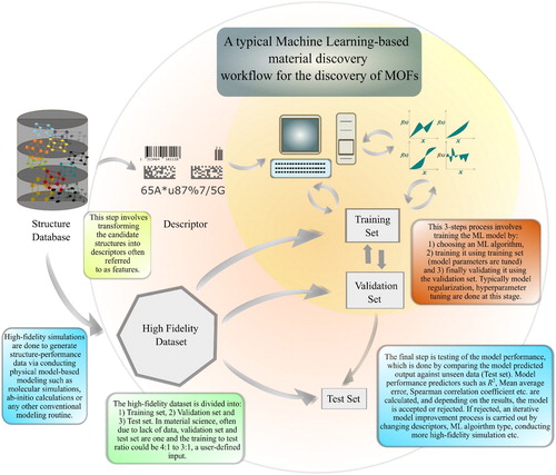
A typical ML-based workflow practiced in the MOF discovery domain is shown in Figure 2. One of the first steps, and perhaps the most critical one, is the selection of molecular descriptors for the system. The descriptor of a MOF is an independent property of a system which is invariant with respect to any transformation which preserves the target property. An example would be, for computational purposes, if we transform the cell size of a material into twice the initial length and assume our target property is melting point, then the descriptor should also remain unaffected with this transformation. As the quantity of interest is melting point, it is not going to be affected by that earlier transformation and so its descriptors should also remain constant. Also, descriptors should be unique and allow for cross-element generalisation. Further, it is also desirable that it should be computationally inexpensive. Programs and libraries such as Dscribe, matminer, pymatgen, RDKit have many such built-in descriptor calculation capabilities [69–72].

Figure 2. (Colour online) A typical machine learning workflow applied to discovery of MOFs. The orange-shaded or the inner region covers the three step process of building an ML model for material discovery (provided the features and training set are available) with the following steps: model selection, model training, and validation. The outer region, coloured in light red, covers the descriptor selection, dataset creation, and model testing parts of the process. This type of inner and outer region representation of the workflow helps us to understand the purpose of the inner region, which is to perfect the model given the dataset and descriptor via traversing these sub-processes: model selection, optimisation, and tuning. The outer region is more focused on handling the dataset and also its best representation in the form of descriptors.

In the next step, we must look at the nature of target property we want to calculate, and based on the atomic scale on which the property depends, a descriptor level should be assigned. Descriptor type and selection hence, are irrevocably linked to the type of property we want to calculate. To explain this further, if our goal is to calculate sub-atomic level properties, selecting a descriptor such as pore size, void fraction, and other gross-level descriptor would not be helpful and we must resort to sub-atomic level features, which are in essence capable of affecting our target property. We can summarise this division in three levels, as was reviewed by Ram Prasad et al. in 2017 [73]:

• Gross-level descriptor – void fraction, density, bulk modulus, glass transition temperature, pore limiting diameter, etc.

• Molecular-fragment level descriptor – SMILEs fingerprint of a molecule, geometric coordinates and topological data, etc. [74].

• Sub-atomic level descriptor – atomic charges, electron density distribution, etc.

After selecting a set of descriptors, we must narrow down the list to the best combination of descriptors for our system, a step which is known as feature selection or feature engineering, since including descriptors having high degree of correlation can hinder the learning process [75,76]. Moreover, feature engineering helps in reducing the total number of descriptors for the model which leads to dimensionality reduction, and thus reduces the cost of building, validating, and testing the ML model [77]. The process also helps in filtering out descriptors which have low-predictive power. Some of the popular ways to conduct feature engineering are:

1. Dimensionality reduction – These methods generally form the broad category for feature selection and can be implemented in a number of ways. Some of them are listed here:

   • Principal Component Analysis (PCA): In this strategy, a new set of dimensions (or features) are created from the old feature space, and then a covariance matrix of all the new features (or dimensions), let us say n, is evaluated from that covariance matrix. Thereafter, individual eigen vectors and eigen values corresponding to each feature are obtained. The principal components are generally obtained by sorting the eigen values in decreasing order, and selecting a p number of components from the variables list. The final p features are thus the principal components and they become the most important features. The eigen values here represent the total share in variance of the dependent variable contributed by that feature. We recommend reading the work by Pearson for further details [78].

   • Linear Discriminant Analysis (LDA): Similar to PCA, LDA tries to create new features from the old feature space but instead of using covariance matrix as a criterion, they create new features which maximises a factor which equates to difference in mean to sum of variances of two features. Thus, the criteria of choosing a new dimension in LDA is the ratio of mean difference to sum of variance, and thus the method can fail when the discriminatory information between features does not reside in the mean [79].

   • Non-negative matrix factorisation (NMF): In this method, the initial matrix of n features with m sample size is represented as the product of two matrices, one of which is $m\times p$, and the other as $p\times n$, where p is much lower than n, the initial number of features. Since its very easy to handle the smaller feature space, NMF leads to dimensionality reduction. Also, the method is called Non-negative matrix factorisation since the initial matrix should only contains positive elements and the generated matrices also have non-negative elements only [80].

   • Others: There are many techniques that are recently becoming useful in the material discovery domain. Some of them are: T-distributed stochastic embedding (t-SNE), Uniform manifold approximation and projection (UMAP), autoencoders, isomap, Kernel-PCA, etc. We recommend reading the 2009 work on comparing different dimensional reduction methods by Maaten and team for further details [81].

2. Filter methods – This section of methods involves eliminating (filtering) those descriptors which have a high degree of correlation with other descriptors or have small influence on the target property [82,83]. Some of the popular methods are F-test, where for testing a single descriptor say $X_i$, two models are constructed, one with a constant, and another with the descriptor and a constant [84]. Next, the least square error between the two models are compared to find the significance of descriptor $X_i$. Finally, based on the performance of $X_i$, it can be accepted or rejected. Another filter-based method is Variance Threshold, where a variance threshold is defined for all the descriptors and only those are accepted which have a variance higher than the limit [85]. Others methods including chi-square test and Fisher score are also used as filter-based methods [86,87].

3. Wrapper methods – There are two standard ways to implement wrapper-based methods, forward search and recursive feature elimination (RFE) [88,89]. Wrapper methods generate many different combinations of descriptors and then builds models for each of those combinations [90]. Forward search works in many steps. The first step begins with (assuming we have n descriptors) creating n different ML models with a single descriptor and then extracting the top descriptor out of n. In the next round, the top descriptor is fixed and now, n−1 models are created with the top descriptor $X_i$ from round 1 fixed, and testing it with all remaining ones. Thereafter, this procedure is repeated until we get a subset of m number of descriptors out of the total n. On the other hand, RFE works by initially building a model with all the n descriptors, and then removing the ones which yield a lower rank in terms of importance, until a m number of descriptors is reached. This is also done via creating a model in each iteration, and performing cross-validation. Although wrapper-type methods are very helpful in finding the most relevant descriptors out of the lot, they are also very expensive since in each iteration of the search a new ML model has to be built, unlike the filter-based methods where the descriptors are ranked based on univariate analysis.

4. Embedded methods – In this category, an ML model is used for descriptor selection in the training part itself, unlike performing cross-validation like the wrapper method [91]. One example is the least absolute shrinkage and selection operator (LASSO) regression model for feature selection where a penalty term is added to the cost function Equation (1(1) $min\frac{1}{2}\sum _{i=1}^n{(y_i-\theta X_i)}^2+\lambda {∥\theta ∥}_1$(1) ) to reduce over-fitting [92]. Those features which performs the best in the regression analysis (i.e. having non-zero values of θ) are retained while others are rejected, as the descriptors with low-predictive power tend to get extremely small values of coefficients (θ). In a similar fashion, tree-based models are also used to select descriptors based on ranking them on their closeness to the root of the tree [93]. (1) $min\frac{1}{2}\sum _{i=1}^n{(y_i-\theta X_i)}^2+\lambda {∥\theta ∥}_1$(1)

Finally, after a set of descriptors are chosen through feature selection process, they are setup as input for developing the ML model. At this stage, the dataset should already have been divided into three sets: training set, validation set, and test set used for model training, validation, and testing, respectively. The objective of all three datasets are different. The training set – consisting of descriptors (representing MOF structures) and associated target variables – serves as an input for building the ML model that we would eventually use later. In the training step, model parameters (weights, constraints, and learning rates) of the ML model are adjusted by minimising the cost function, which relates the error between actual- and model-predicted target variable. Training follows an iterative optimisation of the cost function where the error between model-predicted variable and target variable is minimised by optimising the ML model parameters. After the training is complete, the model is tested against the validation set. In the validation step, model regularisation is done where the model parameters are again optimised to avoid overfitting or underfitting (also known as reduction of variance) [94]. At this juncture, we must state that having a large number of descriptors in the model poses a great likelihood of getting an over-fitted model, and hence feature engineering (described before) is very helpful in avoiding overfitting, inadvertently assisting in model regularisation. Here is the form of a cost function in Equation (2(2) $min\sum _{i=1}^{n}V\left(f\right(X_i),Y_i)+\lambda R\left(f\right(X_i\left)\right)$(2) ) with a regularisation term (a penalty function λ with the regularisation function R). (2) $min\sum _{i=1}^{n}V\left(f\right(X_i),Y_i)+\lambda R\left(f\right(X_i\left)\right)$(2) where the function V is the cost function which relates the difference between actual and predicted properties (based on the descriptors $X_i$). Beyond this step, hyperparameters such as number of neurons, number of layers in an MLP or the number of DTs in an RF routine, are also tuned in the validation step [95,96]. Hyperparameters optimisation involves testing out different combinations of model hyperparameters and selecting the ones which give the best performance. Some of the most common methods for this task are: grid search, random search, evolutionary optimisation, Bayesian optimisation, and gradient-based optimisation [97–101]. These aforementioned steps – model selection, model training, and validation – can be lumped into a three-step process called the ‘inner region’, which we have indicated in the orange-shaded region in Figure 1.

Another region, called the ‘outer’ region concerns with creating, and representing the dataset, and also testing the ML model. After tuning the hyperparameters and performing regularisation in the ‘inner’ region, the model goes through the testing phase where it's final assessment is done. If the model is found satisfactory, it is accepted as a ML model and can potentially replace conventional simulation routines for generating target properties for unseen structures. If not, one must try a new set of descriptors (feature selection) or can change the ML model itself. All these steps fall under the ‘outer region’. This way of dividing the overall computational discovery into two regions serves very important purposes, as ‘inner’ and ‘outer’ regions helps us delineate the data and the model processing parts of the material discovery process which is essential for troubleshooting as well as for methodologically building a robust ML model. The ‘inner’ region is an iterative optimisation process which is put in motion once the ‘outer’ region's tasks are completed, and going forward the model is built and optimised to the extent one can with the sub-processes: trying different ML algorithms, optimising model parameters, tuning hyper-parameters, and performing regularisation. If the model does not end up performing well then another iteration of steps in the ‘outer’ region has to be done in which different descriptors need to be tested. Thus, success and failures in both regions trigger one another, with the loop ending only when one has found a satisfactory model.

It should also be noted that the failure of an ML model can also be due to the lack of data. Since generating structure–property data for materials such as MOFs involves huge computational cost, it is quite possible that the data sampled does not have enough entries. Another possibility is that the sampling space of training set is too narrow which can be analysed by a k-fold cross-validation, where the training and validation set is sampled k different times randomly from the parent dataset, and each time the performance in the $k^{th}$ trial is evaluated to check for consistency [102]. If the performance indicators are consistent for the k trials, one can definitely discard the possibility of a narrow sampling space. Each of the aforementioned should be taken into consideration while building a model and if successful, the model can again be trained with more high-fidelity data to increase its efficiency. In all likelihood, this can prove to be iterative process and hence different descriptors and models must be tested to find the best fit.

3. Machine learning workflows for MOF discovery

In this section, we will highlight some of the recent computational MOF discovery research works, where ML has also been employed. We will cover majorly the descriptors used, the ML workflow employed, and how each ML model fared in the testing phase. In this effort, as we also mentioned earlier, we have to divide this section on the basis of descriptors chosen, first- and second-order descriptors. Although most of the research cited in the section deals with supervised learning examples on MOF-related systems, there are a few exceptions where unsupervised learning has been applied or the material in focus does not exactly qualify as MOF but surely falls under the category of porous material.

3.1. First-order descriptor-based models

In 2015, Simon et al. used RF-based models to predict Xe/Kr separation performance for 670,000 nanoporous structures [103]. The descriptors used were: void fraction ϕ, crystal density ρ, largest free sphere diameter, largest included sphere diameter, surface density ${\rho }_s$, and Voronoi energy descriptor. Firstly, they trained the model on grand canonical monte carlo (GCMC) generated data (15,000 structures) and then tested the RF-based model on candidate structures, followed by an another set of GCMC simulations on high-performing structures. The root mean square error (RMSE) on the training set was 2.21 as compared 1.20 on the test set. Also, they found Voronoi energy descriptor to be the most important feature in the descriptor set (Figure 3) which is shown in Equation (3(3) $E_{\nu }:=\frac{1}{N}\sum _{i=1}^{N}E\left({\nu }_i\right)$(3) ). (3) $E_{\nu }:=\frac{1}{N}\sum _{i=1}^{N}E\left({\nu }_i\right)$(3) where $E\left(\nu \right)$ corresponds to the potential energy of a Xe atom at a point ν in the pore space of the material. The whole pore space is divided into N accessible nodes and $E\left(\nu \right)$ is the energy at the centre of a Voronoi pore landspace. Voronoi energy descriptor is not as much in use as the rest of first-order descriptors but its ease of calculation and growing utility in the nanoporous material space makes it a first-order descriptor.

Figure 3. (Colour online) (a) Selectivity plot of Xe/Kr in the training set with RMSE data [103], (b) Feature importance plot for all descriptors, (c) Selectivity plot of Xe/Kr in the test set with RMSE data, and (d) Distribution of simulated selectivities in the diverse training set compared with a randomly selected set from the dataset. Reprinted with permission from American Chemical Society.

In 2016, Collins et al. built a genetic algorithm-based model (GA) by evolving the functional groups within the pores of a MOF and then they predicted the CO${}_2$ uptake capacity of 1.65 trillion candidate structures, and identified 1035 derivatives and 23 different parent MOFs with high performance in terms of CO${}_2$ capture [104]. In 2016, Aghaji et al., by using DTs and Support Vector Machine (SVM)-based classifier, identified 90% of the high-performing MOFs for CO${}_2$ working capacity and CO${}_2$/CH${}_4$ selectivity for methane separation [48]. The model was trained on a GCMC simulated dataset of 32,450 hypothetical MOFs then SVM classifiers were employed to screen the test set of 290,000 MOFs for only high-performing candidates, followed by applying DTs to find top-candidates for both applications. DT guidelines were based on pore size, void fraction, and surface area. Figure 4 illustrates this DT-based model for assigning a QSPR (quantity structure-performance relationship) score based on the three descriptors. This work by Aghaji and team illustrates how a classification and regression model can be applied in series for screening MOFs.

Figure 4. (Colour online) A DT model for the CO${}_2$ uptake capacity higher than (a) 2 mmol/g, (b) 4 mmol/g of the 32,450 MOFs in the training data set. Each branch represents a QSPR score of 1 or 0 assigned to that MOF if it satisfies a descriptor threshold criteria. The final scores below are averaged QSPR scores [48]. Reprinted with permission from European Journal of Inorganic Chemistry.

Evans et al. in 2017, showed how ML can be used to predict elastic response of zeolites [105]. The descriptors used were geometric features related to local geometry, structure, and porosity of a zeolite. They predicted bulk and shear moduli with an accuracy comparable to that of forcefield-based calculations and used this model on 590,448 hypothetical zeolites. The training set was based on DFT calculations (121 pure Silica zeolites) and they used a gradient boosting regressor (GBR) as the ML model. In a similar fashion, Borboudakis et al. in 2017 employed a customised ML-based tool known as Just Add Data v0.6 (JAD) to estimate CO${}_2$ and H${}_2$ adsorption capacity for 100 known MOFs [106]. They obtained an average Pearson correlation of 0.68 and 0.61 by repeating JAD calculations 100 times for CO${}_2$ and H${}_2$, respectively. JAD is an automated tool that creates a supervised machine learning model and outputs an estimate of its predictive performance as well. For regression problems, JAD employs multiple ML algorithms, such as RF, support vector regression (SVR) using both polynomial and Gaussian kernels and ridge linear regression. They further observed that mean absolute error (MAE) on the test set is lower than the training set for both these cases. Also, when they increased the cut-off threshold of CO${}_2$ and H${}_2$ intake, they found the model performed better (i.e. 85.7% and 80.4% predictions were correct for CO${}_2$ and H${}_2$, respectively). Meanwhile, the model performed poorly on MOFs with low adsorption capacity.

In the same year, Thornton et al. employed MLPs to build a regression model for hydrogen storage. They used the nanoporous materials genome (NMG) database which contains 850,000+ structures including databases such as h-MOFs, CoRE, CSD, and hypothetical zeolites and predicted the room temperature hydrogen storage using the Langmuir adsorption model with input from GCMC simulations [107]. In Figure 5, the net deliverable energy frequency plot for different databases and deliverable energy with respect to void fraction is shown.

Figure 5. (Colour online) The top plot figure shows the log(frequency) with net H${}_2$ delivery capacity for all the databases [107]; while the bottom figure is the net deliverable energy versus void fraction plot. Reprinted with permission from American Chemical Society.

Similarly in 2017, Pardhakhti et al. used customised structural and chemical descriptors to predict methane adsorption performance of a dataset consisting of 130,398 MOFs [108]. They trained the ML model on 8% of this dataset and used RF, Poisson Regression, SVM and DTs to get a correlation coefficient R${}^2$ of 0.98 on the remaining 92% of the MOFs, and an MAE of 7%. The process of training and testing took only 2 h which is remarkable when compared to the time it takes to evaluate such large number of structures with molecular simulations. The structural descriptors used were: void fraction ϕ, surface area, density ρ, dominant pore diameter, maximum pore diameter, interpenetration capacity, and number of interpenetration framework. The chemical descriptors consisted of: number of atoms per units cell, saturation in terms of carbon, metallic percentage, oxygen to metal ratio, electronegative atoms to total atoms ratio, weighted electronegativity per atom, metal type, etc. In Figure 6, we showcase the parity plots for GCMC simulated vs ML-based CH${}_4$ uptake prediction.

Figure 6. (Colour online) The table at the top shows the respective performance of different descriptors for different algorithms in terms of R${}^2$, and root mean square error (RMSE). The bottom figure shows the parity plots for ML-predicted methane uptake versus GCMC simulated data on (a) DT, (b) Poisson regression, (c) SVM, and (d) RF models. The colour scale of the right indicates number of times or number of hMOFs that had the equivalent GCMC and ML result [108]. Reprinted with permission from American Chemical Society.

In the same year, Qiao et al. used PCA, multiple linear regression (MLR) and DTs to asses and determine the relationship between selectivity of adsorption of thiols with respect to air. They performed high-throughput screening of hMOFs and CoRE-MOF database to determine the best material for thiol capture [44,45,109]. The four descriptors used in the model were: void fraction ϕ, isosteric heat of adsorption, largest cavity diameter (LCD), and volumetric surface area (VSA). The initial dataset was first constructed using Monte Carlo simulation on 142,717 MOFs (137,953 from hMOF and 4764 from CoRE-MOFs), and then ML models were used to elucidate the relationship between the selectivity of adsorption of thiols with respect to air.

In 2018, Anderson and team applied DTs to predict the CO${}_2$ capture performance of MOFs which were functionalised with hydroxyl, thiol, cyano, amino, and nitro moieties [110]. The parent MOFs were simulated using DFT and GCMC simulations while the CO${}_2$ uptake of the functionalised MOFs were computed using ML algorithms. After that DTs were used to classify whether parent MOF functionalisation would improve the CO${}_2$ selectivity over N${}_2$ of the parent MOF during exposure to a 15:85/CO${}_2$:N${}_2$ mixture. The descriptors used were: highest bond-dipole moment in the functional group, sum of epsilons in functional groups, most negative charge (MNC) in functional groups, void fraction ϕ of the parent MOF, and topology. In that process, six other ML models, MLP, RF, gradient-boosted machines (GBM), SVM, DT, and MLR, were used to predict CO${}_2$/N${}_2$ selectivity on the functionalised MOFs which were earlier screened by DT model. GBM and MLP gave the highest R${}^2$ as shown in the parity plot in Figure 7, followed by RF, DT, MLR and SVM.

Figure 7. (Colour online) Parity plots for comparing CO${}_2$ selectivity data over N${}_2$ prediction for different ML methods with respect to GCMC calculations [110]. The correlation coefficient R${}^2$ and Spearman ranking correlation coefficient (SRCC) results are also shown for each model. Reprinted with permission from American Chemical Society.

Another work on single-model-based prediction was done by Zhuo et al. in 2018 on inorganic solids [111]. They trained the ML algorithm on 80% of 3896 experimentally reported band gaps and used composition-based descriptors. While they did test several ML algorithms such as k-nearest neighbours (KNN), kernel ridge regression (KRR), and logistic regression (LG), they found support vector regression (SVR) to be the best model. Firstly, a support vector classification (SVC) model was employed to filter out metals, followed by SVR to predict band gaps of inorganic solids. The performance of the classifier was 0.97 area under the receiver operating characteristic (ROC), and an R${}^2$ of 0.90 was obtained for the regression model. Another work in 2018 by Lu et al. was done using band gap as target property for discovering novel hybrid organic-inorganic pervoskites (HOIPs), a class of photovoltaic materials with very high power conversion efficiency (PCE), low-cost synthesis, and tunable band gaps [112]. They used 14 structural descriptors such as p orbital electron X${}_{p-electron}$, ionisation energy, electronegativity ${\chi }_B$, etc. The model employed was gradient boosting regressor (GBR) on a dataset of 5018 hypothetical HOIPs. They obtained a high degree of accuracy in the test set with R${}^2$ and MSE of 0.97 and 0.086, respectively. Also, they used the ML routine as a filter to find potential candidates for more accurate DFT calculations, through which they discovered two HOIPs with excellent band gap and environmental stability. This work presents an example of how ML-based routines can narrow the potential material landscape down to the most promising candidates. Thereafter, higher level methods such as DFT or molecular simulations can be used on the final candidates for accuracy purposes.

In 2018, for finding novel metallic MOFs for application in electronic devices, He et al. created four classification models based on Linear Regression (LR), SVC, MLP, and RF [113]. They trained the ML model on 52,300 inorganic materials (Open Quantum Materials Database (OQMD)), which after testing was employed on potential metallic MOF materials – 2932 MOF structures from the CoRE-MOF database [114]. Forty-five descriptors were employed based on nine elemental properties such as atomic number, group number, period number, density, ionisation energy, and their corresponding statistical quantifiers (i.e. standard mean, standard deviation, geometric mean). Thereafter, classification models were used for a multi-voting decision-making process after processing all the potential metallic MOFs (2937) to select a few high probable candidates for electronic applications, and then a DFT calculation was done to filter out 6 of these novel metallic-MOFs. Metallic MOFs are known for their high electronic conductivity but there are only few in existence and hence finding metallic MOFs through experiments is quite challenging. Also, five of the six MOFs discovered in this work were found to be synthesised earlier and have been reported in literature.

In 2019, Moosavi et al. used data from failed experiments to create an MOF and then used them to build a ML model which was able to capture the chemical intuition behind the MOF synthesis process [115]. They used synthesis conditions data such as DMF, EtOH, or MeOH concentrations, temperature, reactants ratio, reaction time, and microwave power to build a powerful GA tool able to predict progress in crystallinity in subsequent generations. The number of experiments were over 120; some failed and some partly successful. Also, they showed which of the parameters had the most impact on synthesis process. Finally, RF-based decision-making was done to find which operating variables has the most effect on the synthesis process. They obtained H${}_2$O, DMF concentration and reaction temperature, in that order, having the biggest influence on the synthesis process. This presents an example of employing GA in determining the optimum synthesis condition of an MOF.

Recently in 2019, for finding the best MOFs for removal of organosulfurs, Liang and team developed a back propagation neural network (BPNN) and partial least squares (PLS) based model which was trained on NVT-MC simulated dataset of the complete h-MOF database [116]. The descriptors were: LCD, PLD, VSA, void fraction ϕ, Henry's constants K${}_H$, density ρ, and isosteric heat. They found BPNN to perform better than the PLS model. Further, they were able to find eight MOF structures based on a DT analysis, which had high capacity for removal of gaseous organo-sulfurs from high-sour natural gas. Yang et al., in the same year used a PCA analysis to reduce 44 performance metrics of MC and MD generated dataset to only 10 principal components. They used these principal components and structural descriptors (LCD, PLD, VSA, porosity, pore size distribution (PSD) and MOF density), and applied 4 ML algorithms – DT, RF, SVM, and BPNN – to calculate selectivity data for 15 gas mixtures on 6013 CoRE MOF database [117]. Their objective was to test these 4 ML algorithms and analyse the relationship between structural feature descriptors and principal components. They obtained the 30 best MOFs for separation of each of the 15 gas mixtures, and found PLD having the highest weight to the desired performance criteria, and RF as the best model for such pursuits. In 2019, Dureckova et al. predicted CO${}_2$ adsorption and CO${}_2$/H${}_2$ selectivity using GBRs [118]. They employed six geometric descriptors such as surface area, density ρ, void fraction ϕ, and dominant pore size, etc., three AP-RDF-based features (Fernandez et al. [119]), and then trained the model on 80% of 358,500 MOFs structure–property data from GCMC simulations. They found R${}^2$ of 0.944 for CO${}_2$ working capacity, and 0.877 for CO${}_2$/H${}_2$ selectivity. In the same year, Gülsoy and coworkers used DTs and MLPs to extract hidden information from a database containing 2224 MOF structures for CH${}_4$ storage [120]. They found some descriptors to be really useful in determining the MOFs with high storage capacities: i.e. crystal structure and the total degree of saturation. Also, they used a few user-defined descriptors and structural properties and found user-defined descriptors were not sufficient to describe the storage capacities, whereas structural properties led to accurate CH${}_4$-storage predictions with an RMSE of 26.8 (cm${}^3$/g), and R${}^2$ of 0.92 for test set.

In 2019, Wu et al. employed gradient boosting random forest trees (GBRT), SVM and random forest regression (RFR) for methane storage capacity prediction of MOFs on a sample of 130,397 structures-property dataset based on GCMC simulations [121]. The dataset was part of the hMOF database and they divided the 130,397 structure–property data into 7:3 of training and test set. They found RFR to be the best model with an R${}^2$ of 0.9407, followed by GBRT and SVM. In the same year, Shi et al. applied ML-based model to discover best candidates for methanol-MOF pairs in adsorption-driven heat pump applications [122]. They trained four different ML models (SVM, BPNN, RF, and DT) on GCMC calculations (CoRE MOF database with 6013 structures), where it was divided into 7:3 for training and test set. Among these models, RF had the highest R${}^2$ of 0.86 [44], followed by BPNN, DT and SVM. The target variables for the system were coefficient of performance (COP) and ΔW (highest working capacity) and descriptors employed were: LCD, VSA, void fraction ϕ, PLD, density ρ, and heat of adsorption Q${}_{st}$.

Shao et al. in 2020 released a python library known as PiNN, which can create atomic neural networks (MLPs) for molecular systems and, therefore, can predict properties such as energy surfaces, physicochemical properties, etc. [123]. They used two category of descriptors to build MLP-based model. One includes radial and angular terms such as atom-centred symmetry functions and Faber–Christensen–Huang–Lilien-feld representations and the other is expansion of atomic density in terms of orthogonal radial function and spherical harmonics. Both graph convolutional neural network (GCNN) and Behler-Parrinello neural network have been added in this framework and the library has interfaces with both atomic simulation environment (ASE) and Amsterdam Modeling Suite (AMS) [124–126]. Finally, they tested the PiNN library on QM9 dataset containing 50,604 organic molecules and predicted properties like internal energy U${}_0$, and partial charges with very low MAE values [127,128]. In 2020 itself, Rabbani and coworkers published a similar deep learning workflow DeePore for characterising porous materials [129]. The model was developed on feed-forward Convolutional neural network (CNN) and uses 30 descriptors such as pore density, tortuosity, average coordination number, average pore radius, pore sphericity, etc. to predict many morphological, hydraulic, electrical and mechanical properties of the candidate structures. The workflow was validated on a comprehensive porous materials dataset containing 17,700 samples and a wide range of properties were predicted using Deepore. The average R${}^2$ against reference properties obtained was 0.9385, affirming the utility of the workflow developed.

3.2. Second-order descriptor-based models

In 2013, Fernandez et al. reported a new descriptor named atomic property weighted radial distribution function (AP-RDF) for prediction of gas adsorption in MOFs [119]. The descriptor is defined by the following equation: (4) $\mathrm{R}\mathrm{D}{\mathrm{F}}^P\left(R\right)=f\times \sum _{ij}^{\text{all atom pairs}}{P}_i{P}_j{\mathrm{e}}^{-B{(r_{ij}-R)}^2}$(4) where RDF is the radial distribution function, a weighted probability distribution function to find an atom pair in a spherical volume with radius R, r${}_{ij}$ is the minimum image convention distance, f is a scaling factor and P${}_i$/P${}_j$ are the atomic properties used for weighting the RDF function, and B is a smoothing parameter. The properties P${}_i$, can be chosen depending on the chemical information one wants to represent. The properties Fernandez et al. chose were electronegativity, polarizability and van der Waals volume. They showed, from PCA transform of AP-RDF, that the second-order descriptor exhibited good classification of MOF inorganic SBUs (structural building units), geometric properties, and gas uptake capacities. This descriptor also gave reliable prediction of methane and CO${}_2$ uptake capacity for ∼25,000 MOFs and R${}^2$ between 0.70 to 0.82 as shown in Figure 8. It was proposed that the descriptor can be employed as a pre-screening criterion for high-throughput screening of MOFs. It was also observed that the AP-RDF performed much better than first-order descriptors such as pore size, surface area, and void fraction at low pressure, while the latter did better in case of high pressure. In 2014, Fernandez et al. also tested AP-RDF descriptor on a hypothetical MOF database of 324,500 structures for discovery MOF for CO${}_2$ capture [63]. They applied SVM-based classifier and trained the model on 292,050 MOFs from the database. Upon testing the model, they found AP-RDF descriptor-based classifier recovered 945 of the 1000 high-performing MOF from the test set. This further shows the applicability of this particular descriptor in gas storage and separation applications.

Figure 8. (Colour online) Scatter plots for Methane and CO${}_2$ uptake prediction at different pressure based on AR-RDF descriptors versus predicted via GCMC calculations of ∼25000 MOF structures [119]. The correlation coefficient R${}^2$ is shown for all the cases. All the calculation are done at industrial pressure swing adsorption (PSA) conditions. Reprinted with permission from American Chemical Society.

In the same year, First et al. developed an automated computational framework based on optimisation, topological analysis, and graph algorithms to fully characterise the three-dimensional pore structures of MOFs [130]. It was claimed that the methods could identify the portals, channels, and cages of a MOF and describe their geometry and connectivity. Also, they have the capability to calculate pore size distribution (PSD), accessible volume, accessible surface area, PLD, and LCD using the Voronoi decomposition analysis.

In 2016, Fernandez et al. used the k-means clustering and archetypal analysis (AA) to identify significant nano-porous structures for high CO${}_2$ and N${}_2$ uptake capacities [64]. Firstly, k-means clustering was used to group the n MOF structures into k clusters by minimising the within-cluster sum of squares as defined in Equation (5(5) $\mathrm{a}\mathrm{r}{\mathrm{g}}_{s}min\sum _{i=1}^k\sum _{xϵS_i}\parallel x-\mu {\parallel }^2$(5) ), where $S=\{S_1,S_2,\dots ,S_k\}$ represents the k set of clusters and μ is the mean of points in the set $S_i$. (5) $\mathrm{a}\mathrm{r}{\mathrm{g}}_{s}min\sum _{i=1}^k\sum _{xϵS_i}\parallel x-\mu {\parallel }^2$(5) Thereafter, AA was performed on k clusters. AA is a matrix factorisation method to describe the data set variance as a linear combination of a few ‘pure’ archetypes which may not be present in the dataset. In Equation (6(6) $\mathrm{R}\mathrm{S}\mathrm{S}=\sum _{i=1}^n\parallel X_i-\sum _{j=1}^k{\alpha }_{ij}{Z}_i{\parallel }^2$(6) ) and (7(7) $\mathrm{R}\mathrm{S}\mathrm{S}=\sum _{i=1}^n\parallel X_i-\sum _{j=1}^k{\alpha }_{ij}\sum _{i=1}^n{\text{β}}_{ij}{X}_l{\parallel }^2$(7) ), we have the relation of residual sum of squares (RSS) in terms of ‘archetypes’, the X matrix represents the MOF dataset with n structures and m geometrical features and the Z matrix represents archetypal matrix with $k\times m$ size. The algorithm minimises RSS to find the two coefficient matrices α and β (size $n\times k$), which have the following constraints $\sum _{j=1}^k{\alpha }_{ij}=1$ with ${\alpha }_{ij}\ge 0$, and $\sum _{i=1}^n{\text{β}}_{ji}=1$ with ${\text{β}}_{ji}\ge 0$, for α and β, respectively. (6) $\mathrm{R}\mathrm{S}\mathrm{S}=\sum _{i=1}^n\parallel X_i-\sum _{j=1}^k{\alpha }_{ij}{Z}_i{\parallel }^2$(6) (7) $\mathrm{R}\mathrm{S}\mathrm{S}=\sum _{i=1}^n\parallel X_i-\sum _{j=1}^k{\alpha }_{ij}\sum _{i=1}^n{\text{β}}_{ij}{X}_l{\parallel }^2$(7) After extracting the archetypes from the MOF dataset (20% structures from hMOF database), training set was built by systematically including the frameworks with the shortest Euclidean distance for this 20% of the database. After that, a classification model was built with ML algorithms such as MLR, DT, kNN, SVM and MLP to find the MOFs with high CO${}_2$ and N${}_2$ uptake capacities. They tested the method on ∼ 65,000 MOFs and found that the classifier can predict high-performing MOFs (in terms of CO${}_2$ and N${}_2$ gas adsorption performance) with accuracy higher than 94%. This presents an interesting example where an initial dataset was transformed using advanced algorithms to build a more robust training set in terms of variability of input data.

Ohno et al. in 2016, constructed a graph-based kernel function, which was based on the molecular structure, to predict methane storage of an MOF [131]. The method measures the degree of similarity between two structures and can determine the new candidate molecule's pore properties and can predict whether it would yield a methane uptake higher than the prototype molecule from training set. In 2017, Lee et al. reported a new topological-based descriptor which can encapsulate geometric information such as pore size, pore volume, largest included sphere etc. into a molecular fingerprint [132]. In that work, a mathematical quantification of pore shape similarity was done using topological data analysis (TDA). To assign these novel features, one starts with sampling random points on the pore surface of a structure, then spheres are grown around those chosen points in a stepwise fashion and the associated filtered Vietoris-Rips (AFVR) complex is computed by monitoring overlaps between different spheres. The AFVR of each sampled point can be characterised by its 0D, 1D and 2D homology classes (D stands for dimensional), where the lifetime of each class is stored in the 0D, 1D and 2D barcode which is essentially the fingerprint that encapsulates the shape and relevant information about the pore structure. Also, each of the dimensions equates to some key features of the pore landscape; for example, 0D fingerprint gives the connectivity of pores, the 1D descriptor gives number of independent tunnels, while the 2D one captures the radius of the maximum included sphere and ending of each interval in 2D fingerprint indicates radius of cavity. A non-trivial application of the method is to identify geometries with similar pore shapes regardless of chemical composition. To address this, a reference structure (a zeolite) and a set of four most similar structures are considered and their TDA-based descriptor, also named PerH (persistent homology) here, and first-order geometric descriptors were computed. Next, the average distances of the candidates to the original zeolite was calculated for all the testing zeolites, and then the distances from both approaches were compared. It was found that the TDA-based method identified similarity in pore geometry effectively while the first-order descriptor based average distance failed to show any correlation. After that, they used this novel descriptor to divide materials into topological distinct classes by using the pore recognition approach and then screened them based on methane delivery capacity. It was found that 80% of the 130 test structures have a very similar deliverable capacity to those of the original (trained data). A similar study on silicates revealed a 85% concurrence in the deliverable capacity with respect to original training set.

An energy-based descriptor for calculation of hydrogen storage in MOFs was developed by Bucior et al. in 2018 [133]. The descriptor was calculated through MOF-H${}_2$ potential energy surface (PES) by calculating the interaction energy at multiple points on the PES grid-space. They developed a data-driven approach with this descriptor and employed a LASSO regression model to accelerate materials screening and learn structure–property relationships [92]. (8) $\sum _{i=1}^n(y_i-\text{β}{X}_i{)}^2+\lambda \sum _{j=1}^p\left|{\text{β}}_j\right|$(8) Equation (10(10) $f^{-}\left(\overrightarrow{r}\right)\equiv {\left(\frac{\mathrm{\partial }\rho }{\mathrm{\partial }N}\right)}^{-},f^{+}\left(\overrightarrow{r}\right)\equiv {\left(\frac{\mathrm{\partial }\rho }{\mathrm{\partial }N}\right)}^{+}$(10) ) represents the residual sum of squares and a penalty term with a hyperparameter λ, which is the differentiating factor between MLR and LASSO, where $y_i$, and $X_i$ represents input and output vectors of size n, while β is the model parameter vector with size p. The model was trained on 1000 hMOFs H${}_2$ adsorption data and was tested on 1250 hMOFs dataset and later on 4000 MOFs from ToBaCCo database [50–52]. The predicted hydrogen capacity had a MAE of 1.8 g/L and 1.4 g/L, for hMOFs and ToBaCCo, respectively. This workflow of second-order energy descriptor generation has been briefly explained in Figure 9.

Figure 9. (Colour online) The workflow for generating energy descriptor for hydrogen storage [133]. The procedure begins with sampling the potential energy distribution of H${}_2$-MOF interaction in multiple even spaced grid, followed by binning those energy in a histogram. Each of the bins then form an identifier in the energy descriptor of that MOF represented by the input vector $X_i$. Reprinted with permission from American Chemical Society.

While Bucior and team showed us how MOF-adsorbate energetics can be used as a tool of creating descriptors for ML model, in the same year, Sturluson and coworkers performed a new form of data representation which was inspired from image processing. They employed a dimensional reduction technique to create, what they called ‘eigen cages’, from singular value matrix decomposition of porous cage materials [134]. It was demonstrated that a full porous cage can be approximately constructed from these eigen cages as (9) $c_k^T\approx {\overline{c}}^T+\sum _{i=1}^{\nu }{\sigma }_i{u}_i\left[k\right]v_i^T$(9) where the cage $c_k$ is an approximate linear combination of eigen cages $\{v_1,v_2,\dots ,v_{\nu }\}$ with weights formed from a combination of the kth row of the vector $U_{\nu }$ and singular values ${\sigma }_i$. They used it to compare the simulated Xe/Kr selectivity for similar porous cage molecules by t-SNE (t-distributed stochastic neighbour embedding), which is a nonlinear dimensionality reduction technique for modelling high-dimensional objects by a two or three-dimensional point such that similar objects are modelled by nearby points and dissimilar objects are modelled by distant points with high probability (ref. Figure 10).

Figure 10. (Colour online) A latent representation of cages, which is simply the rows of the matrix $U_{\nu }{\mathrm{\Sigma }}_{\nu }$ – which is an equivalent form of Equation (6(6) $\mathrm{R}\mathrm{S}\mathrm{S}=\sum _{i=1}^n\parallel X_i-\sum _{j=1}^k{\alpha }_{ij}{Z}_i{\parallel }^2$(6) )'s right hand side term $U_{\nu }{\mathrm{\Sigma }}_{\nu }\equiv {\sigma }_i{u}_i\left[k\right]$ – embedded into 2D by t-SNE [134]. The coloured points shows the simulated Xe/Kr selectivity of an isolated cage structure at 298 K in an empty box. Furthermore, the points nearby are nearer to each other in the latent cage space and thus are likely to exhibit similar Xe/Kr selectivity while cages marked ‘X’ have too small a window for xenon to enter into the cavity. Reprinted with permission from ACS (American Chemical Society). Further permissions related to the material excerpted should be directed to the ACS.

They observed that cage molecules that are closer in the latent cage space exhibit similar Xe/Kr selectivities, which further reaffirms the potential of this descriptor for encapsulating the features of initial structures into low dimensional ‘eigen cages’.

Another second-order descriptor based on Fukui functions was developed just recently in 2020 by Gusarov et al. for CO${}_2$ reduction reactions [135]. Fukui functions in general indicates changes in the electronic structure of a species in a molecular system during an electrophilic or nucleophilic attack. In essence, Fukui indices reveals the sites in a structure which are most susceptive to lose or gain electrons. (10) $f^{-}\left(\overrightarrow{r}\right)\equiv {\left(\frac{\mathrm{\partial }\rho }{\mathrm{\partial }N}\right)}^{-},f^{+}\left(\overrightarrow{r}\right)\equiv {\left(\frac{\mathrm{\partial }\rho }{\mathrm{\partial }N}\right)}^{+}$(10) where $\rho \left(\overrightarrow{r}\right)$ tells us the electronic density at position $\overrightarrow{r}$, N represents number of electrons and $f^{-}$/$f^{+}$ are electrophilic and nucleophilic fukui indices, respectively. This same idea was used by Gusarov and coworkers to develop a descriptor based on Fukui function projected to the Conolly surface of the system, and then, using linear and multi-variable regression, CO-binding energies were predicted with very high accuracy. The concept can be exploited in modelling MOF-as-catalyst systems and other MOF-related applications where electron-exchange mechanism is at play.

In the previous examples, we defined how descriptors can be made from sub-atomic or gross-level properties. To further elucidate the process of deriving them from different properties, we have listed a few more examples of second-order descriptors in Table 3. Most of these examples consist of descriptors that have been applied to porous materials which means there is an opportunity to test them for MOF-related applications. In theory, a descriptor is just a low-dimensional representation of the molecular structure, which implies the pool for selecting descriptors for MOF is not granted to only those that have been tested for porous materials but also any descriptors is equally eligible to be chosen among thousands. However, just as some computational methods are more suited towards a specific system more than another, in the same vein, descriptors would probably too fit certain materials more than other.

Table 3. A list of some more second-order descriptors with applications and material class.

Descriptor	Properties of interest	Material class	Year
Channel factor and perpendicular	Thermal transport properties	Porous media	2020 [136]
non-uniformity
Local porosity and local mean	Shortest transportation paths	porous materials	2020 [137]
geodesic tortuosity
Geometric landscape within energy–	Gas adsorption	Porous materials	2020 [138]
structure–function(ESF) maps
Persistent homology-based	CH${}_4$ Adsorption	Zeolites	2020 [139]
topological descriptors
PES of the MOF with a probe	CH${}_4$ Adsorption	MOFs	2019 [140]
atom of radius a
Experimentally derived specific	Electric double-layer (EDL)	Nanoporous carbons	2019 [141]
surface area and volume	Capacitance	Material
Fraction of pore size
Pore geometry barcode-based	CH${}_4$ Adsorption	Nanoporous materials	2019 [142]
descriptors: set of distances
from the structure to the most
diverse set in the barcode, and
most important feature of the barcode
Property-labelled materials fragments	Band gap energy,	Inorganic crystals	2017 [143]
	Bulk/shear moduli, Debye
	Temperature, metal/insulator
	Classification and heat capacities
Position of s orbital, number of	CO and NO adsorption	Zeolites	2017 [144]
valence electrons of the active
site and the HOMO-LUMO (highest
occupied molecular orbital and lowest
unoccupied molecular orbital) gap of
the adsorbate
Van der waals surface area	Propensity for structural voids,	Crystalline materials	2016 [145]
	Degree of porosity
Pore landscape descriptors: pore size	Similarity among structures	Crystalline porous	2013 [146]
distribution and stochastic rays		Materials

4. Future of machine learning-based MOF discovery

Given the array of work we have listed, it is evident that ML algorithms can indeed provide useful insights and help reduce computational cost of a simulation study by orders of magnitudes. However, as a tool, it is still novel and there are many chemical systems remaining to be tested for different applications. In fact, ML-based models can help to predict many critical properties for big datasets like hMOFs, CoRE, ToBaCCo, etc. which can serve as a standard for other studies with different properties of interest. In terms of algorithm preference among practitioners, we found RF and MLP-based models (including modified version of deep learning-based models such as CNNs, RNNs) giving excellent prediction for cases when we have large availability of data. It is not surprising that MLP-based models – comprised of multiple hidden layers, edges and neurons with a set of adjustable weights – are inherently flexible for such tasks. A similar role is played by the multiple DTs in case of RF model for mapping complex structure–property relationships. Nonetheless, in case of applications where the data availability is low or it is quite expensive to generate structure–property data, one may look for algorithms like kernel-ridge, gaussian process regressions (GPR), and gradient-boosted decision trees (GBDTs), etc. In a similar spirit, there are efforts being made to test Bayesian learning models in the field of nanoporous materials. Recently, Shih et al. calculated Langmuir isotherm parameters for CO${}_2$ adsorption process using a Bayesian learning algorithm [147]. Following the trend, genetic algorithms have also given reliable prediction when the problems involves hierarchical and step dependent sub-system, such as building a functional group on top of parent molecule or predicting the property of structure via GA as was illustrated by Collins and coworkers by evolving functional groups within pores of an MOF or by Chung and team in 2016, where they genetically modified the linker and nodes of a MOF for multiple generations to find the fittest candidate for CO${}_2$ capture [104,148]. Hence many, if not all, ML algorithms can be applied to the material discovery pipeline depending on their specific advantages and the requirement of the target structure–property relationships.

Another aspect consequential to novel MOF discovery where computational models can provide guidance is predicting synthesisability of a hypothetical structure. Earlier, we referred to the work done by Mossavi et al. where they predicted the conditions for synthesis of a target MOF, HKUST-1, using a robotic synthesiser by using GA [115]. If such insights on synthesis conditions of a MOF can be fed back into a predictive model then we can limit our study to structures having a high probability of being realised in laboratory and thus vastly reducing our search space. There are also parameters such as Tanimoto coefficient which provides a fair idea whether a similar molecule is available commercially or not, but it is based on heuristic rather than physical modelling [149]. It would greatly benefit if we can build DTs which can determine a priori the thermodynamic feasibility to synthesise a target molecule, before simulating the structure–property data [32].

Also, not far from computationally predicting synthesisability, is the goal of inverse design of MOFs – which refers to the process of discovering materials from a desired property. Inverse design is simply the reverse of the current design methodology where instead of generating structures and then calculating its property, the potential structures are generated from the properties of interest one is seeking. The latest work in 2019 by Noh and team on inverse design of solid-state materials provides a perfect example [150,151]. Using variational auto-encoders (VAEs) and deep neural networks, they were able to rediscover existing vanadium oxides compounds, as well as predict many meta-stable structures which can be potentially synthesisable. Also in 2020, Yao and coworkers adopted a similar routine using smVAEs (supramolecular variational encoder) to discover new MOFs with optimised properties for higher capacity and selectivity for CO${}_2$/N${}_2$ and CO${}_2$/CH${}_4$ separation [42]. Both these works shows that generative models (GMs) can serve as a promising way of carrying out material discovery via inverse design, and could also be applied to MOF discovery. Further, as mentioned in the beginning, both these models were based on ‘descriptor free’ ML-based material discovery approach which is a new rising trend in the community.

There is also a scope of utilising new and ongoing developments in neural network-based models for MOF discovery. One such potential model is Equivariant graph neural network (EGNN) [152]. EGNNs, as shown by Satorras and team, are capable of restricting neural networks to only relevant functions by utilising the equivariance in the systems. EGNNs exploits three symmetries – rotational, translations and permutations – as compared to graph neural networks which utilises rotational symmetry. Satorras and team applied the EGNN model on the QM9 dataset and found that EGNN-based model were more computationally efficient than other Equivariant type models, and they showed a clear improvement over the state-of-the-art models for a large number of molecular properties [152]. One benefit EGNN has over traditional MLP-based models is that EGNNs does not require a representation in intermediate layer and can still achieve competitive or better performance.

ML models can also be used to develop computationally inexpensive forcefields where we can use transfer learning, which is a method to gain knowledge from one system and apply to another related system [153]. They can be employed to learn from existing forcefields developed on physical models and then generate a novel forcefield based on the system in consideration. Having the power to accurately calculate forces is crucial for the success of any molecular modelling experiment and hence having such a system would greatly enhance performance of predictive models. A recent work done by Smith et al. serves as a good example, where they created the forcefield known as ANAKIN-ME (Accurate NeurAl networK engINe for Molecular Energies) using neural networks [154] and found comparable accuracy with respect to DFT calculations. The model was employed to learn the training potential energy surfaces and then through transfer learning it was generalised for a new forcefield.

There are also concerns of reproducibility of simulations and many researchers face a challenge just simply replicating published simulation results, sometimes even in the same research group. This is very crucial for the success of any research domain since reproducing and validating science from an earlier study allows one to build new knowledge and expand the known boundaries. Thus, it is very important to keep in mind that every step and procedure in a novel machine learning-based project should be explained and relevant input files and examples are encouraged to be shared with the community. In this vein, efforts such as AiiDA and FireWorks are a step in the right direction to provide a robust workflow for ease of reproducing computational experiments [155,156].

5. Conclusion

In the twenty-first century, many experts claim that data science is the fourth pillar of science along with theory, simulation, and experiments. Thus, as the search for novel porous materials begins to extend beyond the reaches of conventional methods, data science models, based on finding patterns in structure–property relationships holds paramount importance in the field of material discovery. Molecular simulations, both Monte Carlo and molecular dynamics, can take significant time and resources to predict a certain property, due to millions of iterations, equilibration time, solving complex equation based on Newton Laws (in MD), and many more computationally expensive tasks. Hence due to the innumerable possibilities of MOF structures and then dozens of applications of a single MOF, it is essential to leverage the power of ML models to do the intensive work. However, the initial data generation for model initialisation should still befall into the domain of physical modelling techniques.

In this review, we have listed some of the successful cases of ML-based prediction in MOFs and also some descriptors based on structural features like pore size distribution, void fraction ϕ, VSA, PLD, LCD, Voronoi energy, etc. We have also highlighted many novel descriptors (second-order) as well, based on energy surfaces, Fukui functions, topology, and a host of MOF-related properties [119,134], which have been instrumental in reducing dimensions of the modelling problem and thus are key ingredients for building a cheap and reliable ML model. Although there are discussions to be had whether the second-order descriptors are more beneficial and accurate than the first-order, we recommend one should start with the first-order as they are very easy to calculate and apply. Softwares like Zeo++ and Poreblazer are quite popular in extracting some of the first-order descriptors but if the problem demands the need of sophisticated descriptors [157,158], then one should definitely look up for the second-order descriptors, many of which we have reviewed in this work. If the demand exists, one may create a new one, albeit a tailored one for the problem. In the 1980s and 1990s, we witnessed an upsurge of targeted computational methods for different physical and chemical problems, now we are in the wake of a boom of descriptors in the MOF domain and arguably in the larger computational material discovery community. We have also noticed most research works involving ML falls under supervised machine learning, while it is also encouraging to report some unsupervised learning examples such as by Sturluson [134]. As the community starts undertaking bigger systems with more unlabelled data and running into high-dimensional datasets, unsupervised learning-based models will become crucial to tackle those problems. In 2019, an interesting such study was done for the colloidal systems by Adorf et al., where they applied unsupervised SVMs to identify pathways for nucleation and growth of super-cooled liquids [159]. The domains of novel MOFs synthesis and crystal structure prediction also carry similar attributes as the nucleation of super-cooled liquids and hence, the supervised learning approach of Adorf and team could also be utilised for those related domains.

We believe that the future of MOFs – as a material of scientific inquiry and of practical utility – is promising and we will continue to discover new structures and apply them in real-world applications. Many such candidates have already found their place in the society but there are still many unsolved challenges that are essential to the sustenance of modern life as well as for the environment like high-performance catalysts, energy storage, capturing CO${}_2$, CH${}_4$ and CO, renewable energy, drug delivery, proton conduction, electrochemical energy storage, water harvesting, etc. and MOFs can play a pivotal role in tackling them. However, as we have seen with other fields, the discovery of novel methods and applying them to difficult problems is a key process and a continuing one. And hence, there has to be continuous effort in this domain to push the boundaries and untangle the mysteries of nanoporous material discovery field from synthesis to final deployment.

Disclosure statement

No potential conflict of interest was reported by the author(s).

Correction Statement

This article has been republished with minor changes. These changes do not impact the academic content of the article.

References

- Kondo M, Yoshitomi T, Matsuzaka H, et al. Three-dimensional framework with channeling cavities for small molecules: {[M 3(4, 4-bpy) 3(NO 3) 4]·xH 2O} n (M = Co, Ni, Zn). Angew Chem Int Ed Engl. 1997;36:1725–1727.
- Henrietta WL, Jianwei R, Brian N, et al. Hydrogen storage in metal-organic frameworks: a review. Electrochim Acta. 2014;128:368–392.
- Boyd PG, Chidambaram A, García-Díez E, et al. Data-driven design of metal-organic frameworks for wet flue gas CO 2 capture, Nature. 2019;576:253–256.
- Hu Z, Wang Y, Shah BB, et al. CO 2 capture in metal-organic framework adsorbents: an engineering perspective. Adv Sustainable Syst. 2019;3:1800080.
- Pascanu V, González Miera G, Inge AK, et al. Metal-organic frameworks as catalysts for organic synthesis: a critical perspective. J Am Chem Soc. 2019;141(18):7223–7234.
- Lin R-B, Xiang S, Xing H. Exploration of porous metal-organic frameworks for gas separation and purification, Coord Chem Rev. 2019;378:87–103.
- Kreno LE, Leong K, Farha OK, et al. Metal-organic framework materials as chemical sensors. Chem Rev. 2012;112(2):1105–1125.
- Bhardwaj SK, Bhardwaj N, Kaur R, et al. An overview of different strategies to introduce conductivity in metal-organic frameworks and miscellaneous applications thereof. J Mater Chem A. 2018;6:14992–15009.
- Sundriyal S, Kaur H, Bhardwaj SK, et al. Metal-organic frameworks and their composites as efficient electrodes for supercapacitor applications. Coord Chem Rev. 2018;369:00.
- Xing X-S, Fu Z-H, Zhang N-N, et al. High proton conduction in an excellent water-stable gadolinium metal-organic framework. Chem Commun. 2019;55:1241–1244.
- Ramaswamy P, Wonga NE, Shimizu GKH. MOFs as proton conductors-challenges and opportunities. Chem Soc Rev. 2014;43:5913–5932.
- So MC, Wiederrecht GP, Mondloch JE, et al. Metal-organic framework materials for light-harvesting and energy transfer. Chem Commun. 2015;51:3501–3510.
- Wang L, Zheng M, Xie Z. Nanoscale metal-organic frameworks for drug delivery: a conventional platform with new promise. J Mater Chem B. 2018;6:707–717.
- Gandara-Loe J, Ortuño-Lizarán I, Fernández-Sanchez L, et al. Metal-Organic frameworks as drug delivery platforms for ocular therapeutics. ACS Appl Mater Interfaces. 2019;11(2):1924–1931.
- Omar KF, Ibrahim E, Nak Cheon J, et al. Metal-Organic framework materials with ultrahigh surface areas: is the sky the limit? J Am Chem Soc. 2012;134(36):15016–15021.
- Furukawa H, Ko N, Go YB, et al. Ultrahigh porosity in metal-organic frameworksScience. 2010;329:424–428.
- Farha OK, Yazaydın AO, Eryazici I, et al. De novo synthesis of a metal-organic framework material featuring ultrahigh surface area and gas storage capacitiesNat Chem. 2010;2:944–948.
- Koh K, Wong-Foy AG, Matzger AJ. A porous coordination copolymer with over 5000 m 2/g BET surface areaJ Am Chem Soc. 2009;131:4184–4185.
- Yan Y, Telepeni I, Yang S, et al. Metal-Organic polyhedral frameworks: high H 2 adsorption capacities and neutron powder diffraction studiesAm Chem Soc. 2010;132:4092–4094.
- Klein N, Senkovska I, Baburin IA, et al. Route to a family of robust, non-interpenetrated metal-organic frameworks with pto-like topologyChem Eur J. 2011;17:13007.13016
- Furukawa H, Miller MA, Yaghi OM. Independent verification of the saturation hydrogen uptake in MOF-177 and establishment of a benchmark for hydrogen adsorption in metal-organic frameworksJ Mater Chem. 2007;17:3197.
- An J, Farha OK, Hupp JT, et al. Metal-adeninate vertices for the construction of an exceptionally porous metal-organic frameworkNat Commun. 2012;3:604.
- Ferey G, Mellot-Draznieks C, Serre C, et al. A chromium terephthalate-based solid with unusually large pore volumes and surface areaScience. 2005;309:2040.2042
- Koh K, Wong-Foy AG, Matzger A. A porous coordination copolymer with over 5000 m 2/g BET surface area. J Angew Chem Int Ed. 2008;47:677.
- Sumida K, Hill MR, Horike S, et al. Synthesis and hydrogen storage properties of Be12 (OH) 12 (1, 3, 5-benzenetribenzoate) 4. J Am Chem Soc. 2009;131:15120.
- Zhao D, Yuan D, Sun D, et al. Stabilization of metal-organic frameworks with high surface areas by the incorporation of mesocavities with microwindows. J Am Chem Soc. 2009;131:9186.
- Li WJ, Lu J, Gao SY, et al. Electrochemical preparation of metal-organic framework films for fast detection of nitro explosives. J Mater Chem A. 2014;2:19473.
- Korean J. Synthesis of metal-organic frameworks: a mini review. Chem Eng. 2013;30(9):1667–1680.
- Zou F, Yu R, Li R, et al. Microwave-assisted synthesis of HKUST-1 and functionalized HKUST-1-@H3PW12O40: selective adsorption of heavy metal ions in water analyzed with synchrotron radiation. Chemphyschem. 2013 Aug 26;14(12):2825–2832. DOI: 10.1002/cphc.201300215
- Dey C, Kundu T, Biswal BP, et al. Crystalline metal-organic frameworks (MOFs): synthesis, structure and function. Acta Crystallogr B Struct Sci Cryst Eng Mater. 2014 Feb;70(Pt 1):3–10. DOI: 10.1107/S2052520613029557. Epub 2013 Dec 10. PMID: 24441122.
- Notman N. MOFs find a use. Chemistry World 2017 [cited 2019 Apr 1]. Available from: https://www.chemistryworld.com/features/mofs-find-a-use/2500508.article
- Anderson R, Gómez-Gualdrón DA. Large-scale free energy calculations on a computational metal-Organic frameworks database: toward synthetic likelihood predictions. Chem Mater. 2020;32(19):8106–8119.
- Arni S, Melanie T, Huynh A, et al. The role of molecular modelling and simulation in the discovery and deployment of metal-organic frameworks for gas storage and separation. Mol Simul. 2019;45(14–15):1082–1121.
- Michie D. “Memo” functions and machine learning (reprinted from nature, vol. 218, no. 5136, pp. 19–22, april 6, 1968). Available from: https://stacks.stanford.edu/file/druid:jt687kv7146/jt687kv7146.pdf
- Svetnik V, Liaw A, Tong C, et al. Random forest: a classification and regression tool for compound classification and QSAR modeling. J Chem Inf Comput Sci. 2003 Nov–Dec;43(6):1947–1958.
- Whitley D. A genetic algorithm tutorial. Stat Comput. 1994;4:65–85.
- Tim H, Leorey M, Marcus O, et al. Artificial neural network models for forecasting and decision making. Int J Forecast. 1994;10(1):5–15.
- LeCun Y, Bengio Y, Hinton G. Deep learning. Nature. 2015;521:436.
- Goh GB, Hodas NO, Vishnu A. Deep learning for computational chemistry. J Comput Chem. 2017;38:1291–1307.
- Gen M, Lin L. Genetic algorithms. In: Wah BW, editor. Wiley encyclopedia of computer science and engineering. New York (NY): Wiley-Interscience; 2007. p. 1–15. Available from: https://onlinelibrary.wiley.com/doi/abs/10.1002/9780470050118.ecse169.
- Yao Z, Sanchez-Lengeling B, Bobbitt NS, et al. Inverse design of nanoporous crystalline reticular materials with deep generative models. ChemRxiv. 2020. Available from: https://doi.org/10.26434/chemrxiv.12186681.v1
- Moghadam PZ, Li A, Wiggin SB, et al. Development of a cambridge structural database subset: a collection of metal-organic frameworks for past, present, and future. Chem Mater. 2017;29(7):2618–2625.
- Chung YG, Haldoupis E, Bucior BJ, et al. Advances, updates, and analytics for the computation-ready, experimental metal-organic framework database: CoRE MOF 2019. J Chem Eng Data. 2019;64(12):5985–5998.
- Wilmer CE, Leaf M, Lee CY, et al. Large-scale screening of hypothetical metal-organic frameworks. Nat Chem. 2011 Nov 6;4(2):83–89.
- Moosavi SM, Nandy A, Jablonka KM, et al. Understanding the diversity of the metal-organic framework ecosystem. Nat Commun. 2020;11:4068.
- Shi Z, Yang W, Deng X, et al. Machine-learning-assisted high-throughput computational screening of high performance metal-organic frameworks. Mol Syst Des Eng. 2020;5:725–742.
- Aghaji MZ, Fernandez M, Boyd PG, et al. Quantitative structure-property relationship models for recognizing metal organic frameworks (MOFs) with high CO2 working capacity and CO2/ CH4 selectivity for methane purification. Eur J Inorg Chem. 2016;2016:4505–4511.
- Moghadam PZ, Li A, Liu XW, et al. Targeted classification of metal-organic frameworks in the Cambridge structural database (CSD). Chem Sci. 2020; 11(32):8373–8387. Advance Article
- Colón YJ, Gómez-Gualdrón DA, Snurr RQ. Topologically guided, automated construction of metal-organic frameworks and their evaluation for energy-related applications. Crystal Growth & Design. 2017;17(11):5801–5810.
- Gómez-Gualdrón DA, Colón YJ, Zhang X, et al. Evaluating topologically diverse metal-organic frameworks for cryo-adsorbed hydrogen storage. Energy Environ Sci. 2016;9:3279–3289.
- Andersona R, Gómez-Gualdrón DA. Increasing topological diversity during computational “synthesis” of porous crystals: how and why. CrystEngComm. 2019;21:1653–1665.
- Bao Y, Martin RL, Haranczyk M, et al. In silico prediction of MOFs with high deliverable capacity or internal surface area. Phys Chem Chem Phys. 2015 May 14;17(18):11962–11973.
- Bao Y, Martin RL, Simon CM, et al. In silico discovery of high deliverable capacity metal-organic frameworks. J Phys Chem C. 2015;119(1):186–195.
- Gomez-Gualdron DA, Gutov OV, Krungleviciute V, et al. Computational design of metal-organic frameworks based on stable zirconium building units for storage and delivery of methane. Chem Mater. 2014;26(19):5632–5639.
- Martin RL, Lin LC, Jariwala K, et al. Mail-order metal-organic frameworks (MOFs): designing isoreticular MOF-5 analogues comprising commercially available organic molecules. J Phys Chem C. 2013;117(23):12159–12167.
- Samuel AL. Some studies in machine learning using the game of checkers. IBM J Res Dev. July 1959;3(3):210–229.
- Das A, Jain A. Indexing the world wide web: The journey so far. Google Inc., USA. Available from: https://static.googleusercontent.com/media/research.google.com/en//pubs/archive/37043.pdf
- Dada EG, Bassi JS, Chiroma H, et al. Machine learning for email spam filtering: review, approaches and open research problems. Heliyon. 2019;5(6):e01802.
- Covington P, Adams J, Sargin E. Deep neural networks for YouTube recommendations. CA: Google Mountain View. Available from: https://storage.googleapis.com/pub-tools-public-publication-data/pdf/45530.pdf
- Gomez-Uribe CA, Hunt N. The Netflix recommender system: algorithms, business value, and innovation. ACM Trans Manage Inf Syst. 2016;6(4):13. Article (January 2016), 19 pages. Available from: https://doi.org/10.1145/2843948
- Singh A, Thakur N, Sharma A. A review of supervised machine learning algorithms. 2016 3rd International Conference on Computing for Sustainable Global Development (INDIACom); New Delhi: 2016. p. 1310–1315.
- Fernandez M, Boyd PG, Daff TD, et al. Rapid and accurate machine learning recognition of high performing metal organic frameworks for CO 2 capture. J Phys Chem Lett. 2014;5(17):3056–3060.
- Fernandez M, Barnard AS. Geometrical properties can predict CO2 and N2 adsorption performance of metal-organic frameworks (MOFs) at low pressure. ACS Comb Sci. 2016;18(5):243–252.
- Sivaraman G, Jackson NE, Sanchez-Lengeling B, et al. A diversified machine learning strategy for predicting and understanding molecular melting points. 2019.
- Venkatraman V, Evjen S, Knuutila HK, et al. Predicting ionic liquid melting points using machine learning. J Mol Liq. 2018;264:318–326.
- Wu H, Fang WZ, Wang Q, et al. Predicting effective diffusivity of porous media from images by deep learning. Sci Rep. 2019;9:20387.
- Muñoz-Gil G, Garcia-March MA, Manzo C, et al. Single trajectory characterization via machine learning. New J Phys. 2020;22:013010.
- Himanen L, Marc OJ, Jäger EV, et al. DScribe: library of descriptors for machine learning in materials science. Comput Phys Commun. 2020;247:106949.
- Ward L, Dunn A, Faghaninia A, et al. Matminer: an open source toolkit for materials data mining. Comput Mater Sci. 2018;152:60–69.
- Ong SP, Richards WD, Jain A, et al. Python materials genomics (pymatgen): a robust, open-source python library for materials analysis. Comput Mater Sci. 2013;68:314–319.
- RDKit: Open-source cheminformatics. Available from: http://www.rdkit.org.
- Ramprasad R, Batra R, Pilania G, et al. Machine learning in materials informatics: recent applications and prospects. npj Comput Mater. 2017;3:54.
- Quirós M, Gražulis S, Girdzijauskaitė S, et al. Using SMILES strings for the description of chemical connectivity in the crystallography open database. J Cheminform. 2018;10:23.
- Turner CR, Fuggetta A, Lavazza L, et al. A conceptual basis for feature engineering. J Syst Soft. 1999;49(1):1999.
- Feature engineering for machine learning: principles and techniques for data scientists. In: Zheng A, Casari A, editors. 2018. Available from: books.google.com.
- Dimensionality reduction: a comparative review. van der Maaten L, Postma E, van den Herik J, editors. TiCC, Tilburg University; October 26, 2009.
- Pearson K. LIII. on lines and planes of closest fit to systems of points in space. Lond Edinb Dublin Philos Mag J Sci. 1901;2(11):559–572. DOI: 10.1080/14786440109462720.
- Mika S, Ratsch G, Weston J, et al. Fisher discriminant analysis with kernels. Neural Networks for Signal Processing IX: Proceedings of the 1999 IEEE Signal Processing Society Workshop (Cat. No.98TH8468); Madison (WI): 1999. p. 41–48.
- Ren B, Pueyo L, Zhu GB. Non-negative matrix factorization: robust extraction of extended structures. Astrophys J. 2018;852(2):104.
- Dimensionality reduction: a comparative review. In: van der Maaten L, Postma E, van den Herik, J, editors. Source: Tilburg University; TiCC TR 2009-005. 2009.
- Ambusaidi MA, He X, Nanda P, et al. Building an intrusion detection system using a filter-based feature selection algorithm. IEEE Trans Comput. 1 Oct 2016;65(10):2986–2998.
- Sánchez-Maroño N, Alonso-Betanzos A, Tombilla-Sanromán M. Filter methods for feature selection – a comparative study. Intelligent Data Engineering and Automated Learning – IDEAL 2007. p. 178–187.
- Asaithambi S. Why, how and when to apply feature selection. https://towardsdatascience.com/why-how-and-when-toapply-feature-selection-e9c69adfabf2#:∼:text=F%20Test,a%20constant%20and%20a%20feature.
- Sadeghyan S. A new robust feature selection method using variance-based sensitivity analysis. arXiv:1804.05092.
- Jin X, Xu A, Bie R, et al. Machine learning techniques and chi-square feature selection for cancer classification using sage gene expression profiles. Data mining for biomedical applications. 2006.
- Gu Q, Li Z, Han J. Generalized Fisher score for feature selection. 2012. arXiv:1202.3725.
- Pirgazi J, Alimoradi M, Abharian TE, et al. An efficient hybrid filter-wrapper metaheuristic-based gene selection method for high dimensional datasets. Sci Rep. 2019;9:18580.
- Brownlee J. Recursive feature elimination (RFE) for feature selection in Python. Available from: https://machinelearningmastery.com/rfe-feature-selection-in-python/
- Somol P, Baesens B, Pudil P, et al. Filter-versus wrapper-based feature selection for credit scoring. Int J Intell Syst. 2005;20:985–999.
- Lal TN, Chapelle O, Weston J, et al. Embedded methods. Feature extraction. p 137–165.
- Gauraha N. Introduction to the LASSO. Reson. 2018;23:439–464. Available from: https://doi.org/10.1007/s12045-018-0635-x
- Yashkov IB. Feature selection using decision trees in the problem of JSM classification. Autom Doc Math Linguist. 2014;48:6–11. Available from: https://doi.org/10.3103/S000510551401004X
- Wan L, Zeiler M, Zhang S. Regularization of neural networks using dropconnect. Proceedings of the 30th international conference on Machine Learning; 2013 Jun 16–21; Atlanta (GA): ACM; 2013. p. 1058–1066.
- Claesen M, De Moor B. Hyperparameter search in machine learning. 2015. arXiv:1502.02127.
- Bergstra J, Bardenet R, Bengio Y, et al. Algorithms for hyper-parameter optimization (PDF). Advances in neural information processing systems. 2011.
- Bergstra J, Bengio Y. Random search for hyper-Parameter optimization (PDF). J Mach Learn Res. 2012;13:281–305.
- Wang Z, Hutter F, Zoghi M. Bayesian optimization in a billion dimensions via random embeddings. J Artif Intell Res. 2016;55:361–387. arXiv:1301.1942. DOI: 10.1613/jair.4806
- Hutter F, Hoos H, Leyton-Brown K. Sequential model-based optimization for general algorithm configuration (PDF), learning and intelligent optimization. Lecture notes computer science. 2011;6683:507–523. CiteSeerX 10.1.1.307.8813, DOI: 10.1007/978-3-642-25566-340, ISBN 978-3-642-25565-6.
- Franceschi L, Donini M, Frasconi P, et al. Forward and reverse gradient-based hyperparameter optimization (PDF). Proceedings of the 34th International Conference on Machine Learning; 2017. arXiv:1703.01785.
- Jaderberg M, Dalibard V, Osindero S, et al. Population based training of neural networks. 2017. arXiv:1711.09846
- Jung Y, Hu J. A K-fold averaging cross-validation procedure. J Nonparametr Stat. 2015;27(2):167–179. DOI: 10.1080/10485252.2015.1010532. Epub 2015 Feb 26. PMID: 27630515; PMCID: PMC5019184.
- Simon CM, Mercado R, Schnell SK, et al. What are the best materials to separate a xenon/krypton mixture?. Chem Mater. 2015;27(12):4459–4475.
- Collins SP, Daff TD, Piotrkowski SS, et al. Materials design by evolutionary optimization of functional groups in metal-organic frameworks. Sci Adv. 23 Nov 2016;2(11):e1600954.
- Evans JD, Coudert F-X. Predicting the mechanical properties of zeolite frameworks by machine learning. Chem Mater. 2017;29(18):7833–7839.
- Borboudakis G, Stergiannakos T, Frysali M, et al. Chemically intuited, large-scale screening of MOFs by machine learning techniques. npj Comput Mater. 2017;3:40.
- Thornton AW, Simon CM, Kin J, et al. Materials genome in action: identifying the performance limits of physical hydrogen storage. Chem Mater. 2017;29(7):2844–2854.
- Pardakhti M, Moharreri E, Wanik D, et al. Machine learning using combined structural and chemical descriptors for prediction of methane adsorption performance of metal organic frameworks (MOFs). ACS Comb Sci. 2017;19(10):640–645.
- Qiao Z, Xu Q, Cheetham AK, et al. High-throughput computational screening of metal-organic frameworks for thiol capture. J Phys Chem C. 2017;121(40):22208–22215.
- Anderson R, Rodgers J, Argueta E, et al. High-throughput computational screening of metal-organic frameworks for thiol capture. Chem Mater. 2018;30(18):6325–6337.
- Zhuo Y, Mansouri Tehrani A, Brgoch J. Predicting the band gaps of inorganic solids by machine learning. J Phys Chem Lett. 2018;9(7):1668–1673.
- Lu S, Zhou Q, Ouyang Y, et al. Accelerated discovery of stable lead-free hybrid organic-inorganic perovskites via machine learning. Nat Commun. 2018;9:3405.
- He Y, Cubuk ED, Allendorf MD, et al. Metallic metal-organic frameworks predicted by the combination of machine learning methods and ab initio calculations. J Phys Chem Lett. 2018;9(16):4562–4569.
- Kirklin S, Saal JE, Meredig B, et al. The open quantum materials database (OQMD): assessing the accuracy of DFT formation energies. npj Comput Mater. 2015;1:15010.
- Moosavi SM, Chidambaram A, Talirz L, et al. Capturing chemical intuition in synthesis of metal-organic frameworks. Nat Commun. 2019;10:539.
- Liang H, Yang W, Peng F. Combining large-scale screening and machine learning to predict the metal-organic frameworks for organosulfurs removal from high-sour natural gas. APL Mater. September 2019;7(9):091101.
- Yang W, Liang H, Peng F, et al. Computational screening of metal-Organic framework membranes for the separation of 15 gas mixtures. Nanomaterials. 2019 Mar 20;9(3):467.
- Dureckova H, Krykunov M, Aghaji MZ, et al. Robust machine learning models for predicting high CO2 working capacity and CO2/H2 selectivity of gas adsorption in metal organic frameworks for precombustion carbon capture. J Phys Chem C. 2019;123(7):4133–4139.
- Fernandez M, Trefiak NR, Woo TK. Atomic property weighted radial distribution functions descriptors of metal-organic frameworks for the prediction of gas uptake capacity. J Phys Chem C. 2013;117(27):14095–14105.
- Gülsoy Z, Sezginel KB, Uzun A, et al. Analysis of CH4 uptake over metal-Organic frameworks using data-Mining tools. ACS Comb Sci. 2019;21(4):257–268.
- Wu X, Xiang S, Su J, et al. Understanding quantitative relationship between methane storage capacities and characteristic properties of metal-Organic frameworks based on machine learning. J Phys Chem C. 2019;123(14):8550–8559.
- Shi Z, Liang H, Yang W, et al. Machine learning and in silico discovery of metal-organic frameworks: methanol as a working fluid in adsorption-driven heat pumps and chillers. Chem Eng Sci. 2020;214:115430.
- Shao Y, Hellström M, Mitev PD. PiNN: a python library for building atomic neural networks of molecules and materials. J Chem Inf Model. 2020;60(3):1184–1193.
- Behler J, Parrinello M. Generalized neural-network representation of high-dimensional potential-energy surfaces. Phys Rev Lett. 2 April 2007;98:146401. Published
- Larsen AH, Mortensen JJ, Blomqvist J, et al. The atomic simulation environment-a python library for working with atoms. J Phys: Condens Matter. 2017;29:273002.
- Velde G, Bickelhaupt FM, Baerends EJ, et al. Chemistry with ADF. J Comput Chem. 2001;22:931–967. Availalbe from: https://doi.org/10.1002/jcc.1056.
- Ruddigkeit L, van Deursen R, Blum LC, et al. Enumeration of 166 billion organic small molecules in the chemical universe database GDB-17. J Chem Inf Model. 2012;52:2864–2875.
- Ramakrishnan R, Dral PO, Rupp M. Quantum chemistry structures and properties of 134 kilo molecules. Sci Data. 2014;1:140022.
- Rabbani A, Babaei M, Shams R, et al. DeePore: a deep learning workflow for rapid and comprehensive characterization of porous materials. Adv Water Resour. 2020;146:103787. ISSN 0309-1708. Available from: https://doi.org/10.1016/j.advwatres.2020.103787
- First EL, Floudas CA. MOFomics: computational pore characterization of metal-organic frameworks. Microporous Mesoporous Mater. 2013;165:32–39.
- Ohno H, Yusuke Mukae Y. Machine learning approach for prediction and search: application to methane storage in a metal-organic framework. J Phys Chem C. 2016;120(42):23963–23968.
- Lee Y, Barthel S, Dłotko P, et al. Quantifying similarity of pore-geometry in nanoporous materials. Nat Commun. 2017;8:15396.
- Bucior BJ, Bobbitt NS, Islamoglu T, et al. Energy-based descriptors to rapidly predict hydrogen storage in metal-organic frameworks. Mol Syst Des Eng. 2019;4:162–174.
- Sturluson A, Huynh MT, York AHP, et al. Eigencages: learning a latent space of porous cage molecules. ACS Cent Sci. 2018;4(12):1663–1676.
- Gusarov S, Stoyanov SR, Siahrostami S. Development of Fukui function based descriptors for a machine learning study of CO2 reduction. J Phys Chem C. 2020;124(18):10079–10084.
- Wei H, Bao H, Ruan X. Machine learning prediction of thermal transport in porous media with physics-based descriptors. Int J Heat Mass Transf. 2020;160:120176. ISSN 0017-9310
- Neumann M, Machado Charry E, Zojer K, et al. On variability and interdependence of local porosity and local tortuosity in porous materials: a case study for sack paper. Methodol Comput Appl Probab. 2020; 1–15. Available from: https://doi.org/10.1007/s11009-019-09761-1:
- Moosavi SM, Xu H, Chen L, et al. Geometric landscapes for material discovery within energy-structure-function maps. Chem Sci. 2020;11:5423–5433.
- Krishnapriyan AS, Haranczyk M, Morozov D. Topological descriptors help predict guest adsorption in nanoporous materials. J Phys Chem C. 2020;124(17):9360–9368.
- Fanourgakis GS, Gkagkas K, Tylianakis E, et al. A robust machine learning algorithm for the prediction of methane adsorption in nanoporous materials. J Phys Chem A. 2019;123(28):6080–6087.
- Käärik M, Arulepp M, Käärik M, et al. Characterization and prediction of double-layer capacitance of nanoporous carbon materials using the quantitative nano-structure-property relationship approach based on experimentally determined porosity descriptors. Carbon. 2020;158:494–504.
- Zhang X, Cui J, Zhang K, et al. Machine learning prediction on properties of nanoporous materials utilizing pore geometry barcodes. J Chem Inf Model. 2019;59(11):4636–4644.
- Isayev O, Oses C, Toher C, et al. Universal fragment descriptors for predicting properties of inorganic crystals. Nat Commun. 2017;8:15679. Available from: https://doi.org/10.1038/ncomms15679
- Evans JD, Huang DM, Haranczyk M, et al. Computational identification of organic porous molecular crystals. CrystEngComm. 2016;18:4133–4141.
- Goltl F, Müller P, Uchupalanun P, et al. Developing a descriptor-based approach for CO and NO adsorption strength to transition metal sites in zeolites. Chem Mater. 2017;29(15):6434–6444.
- Pinheiro M, Martin RL, Rycroft CH, et al. Characterization and comparison of pore landscapes in crystalline porous materials. J Mol Graphics Model. 2013;44:208–219. ISSN 1093-3263.
- Shih C, Park J, Sholl DS, et al. Hierarchical Bayesian estimation for adsorption isotherm parameter determination. Chem Eng Sci. 2020;214:115435.
- Chung YG, Gómez-gualdrn DA, Li P, et al. In silico discovery of metal-organic frameworks for precombustion CO2 capture using a genetic algorithm. Sci Adv. 14 OCT 2016;2:E1600909.
- Bajusz D, Rácz A, Héberger K. Why is Tanimoto index an appropriate choice for fingerprint-based similarity calculations?. J Cheminform. 2015 May 20;7:20.
- Noh J, Kim J, Stein HS, et al. Inverse design of solid-State materials via a continuous representation. Matter. 2019;1(5):1370–1384.
- Tutorial on variational Autoencoders Carl Doersch. 2016 Tutorial of arxiv.
- E(n) Equivariant graph neural networks. In: Satorras VG, Hoogeboom E, Welling M, editors. arXiv:2102.09844v1.
- Ma R, Colón YJ, Luo T. Transfer learning study of gas adsorption in metal-Organic frameworks. ACS Appl Mater Interfaces. 2020;12(30):34041–34048.
- Smith JS, Isayev O, Roitberg AE. ANI-1: an extensible neural network potential with DFT accuracy at force field computational cost. Chem Sci. 2017;8:3192–3203.
- Pizzi G, Cepellotti A, Sabatini R, et al. AiiDA: automated interactive infrastructure and database for computational science. Comput Mater Sci. 2015;111: DOI: 10.1016/j.commatsci.2015.09.013.
- Jain A, Ong SP, Chen W, et al. FireWorks: a dynamic workflow system designed for high-throughput applications. Concurr Comput: Pract Exper. 17 December 2015;27:5037–5059.
- Willems TF, Rycroft CH, Kazi M. Algorithms and tools for high-throughput geometry-based analysis of crystalline porous materials. Microporous Mesoporous Mater. 2012;149(1):134–141.
- Sarkisov L, Harrison A. Computational structure characterisation tools in application to ordered and disordered porous materials. Mol Simul. 2011;37(15):1248–1257.
- Adorf CS, Moore TC, Melle YJU, et al. Analysis of self-assembly pathways with unsupervised machine learning algorithms. J Phys Chem B. 2020;124(1):69–78.