Deciphering the structural and functional impact of Q657L mutation in NLRC4 using computational methods

ABSTRACT

The NLR family caspase recruitment domain-containing protein 4 (NLRC4) inflammasome regulates the inflammatory response. Upregulation of NLRC4 inflammasome has been associated with bacterial infections, cancers, and autoinflammatory disorders (AIDs). The Q657L mutation in the NLRC4 causes AID. However, the structural change upon Q657L mutation at the atomic level has not been clearly understood. In this study, we employed in silico predictions along with molecular dynamics (MD) simulations of the homology modelled human wild-type and mutant NLRC4 structures in the resting and activated state to investigate the impact of Q657L mutation on the structural and dynamic changes of NLRC4 protein. The Q657L mutation was predicted to be deleterious by various in silico prediction tools. The MD simulation results demonstrated that the mutation increased the stability of the compactly folded structure and decreased flexibility in the resting state. In the activated state, the stably folded mutant structure had increased solvent accessible surface area, intermolecular hydrogen bonds and binding pocket volume. In addition, the principal component analysis showed that the mutant structures had reduced dynamics in both states. These findings provide insights into structural and dynamic changes of NLRC4 protein due to Q657L mutation at the atomic level.

KEYWORDS:

• NLRC4
• inflammasome
• Q657L mutation
• homology modelling
• molecular dynamics simulation

1. Introduction

Autoinflammatory disorders (AIDs) are caused by dysregulation in the innate inflammatory responses, resulting in recurrent fevers and systemic inflammation [1]. More than 40 genes are associated with AIDs [2]. Any mutation within these genes might lead to aberrant inflammasome activation, protein misfolding, excessive NF-κB activation, interferonopathies, or inappropriate complement activation [3]. It is inferred that the aberrant inflammasome activation may be due to a mutation in the NLRC4 (NLR family caspase recruitment domain-containing protein 4). NLRC4 is located on the short arm of chromosome 2 (2p22.3), which encodes for 1024 amino acids. NLRC4 inflammasome activation promotes caspase-1-dependent pro-inflammatory cytokine processing and inflammatory cell death [4].

The NLRC4 protein consists of six domains: caspase-activation and recruitment domain (CARD), nucleotide-binding domain (NBD), helical domain 1 (HD1), winged-helix domain (WHD), helical domain 2 (HD2) and leucine-rich repeats (LRR) domain. The crystal structure of mouse NLRC4 with a truncated CARD was solved by X-ray crystallography in 2013. In its resting state, an ADP molecule is bound to the NBD and WHD to stabilise the closed conformational structure preventing self-oligomerisation [5]. The NLRC4 conformational transition happens with the exchange of ADP in the inactive state to ATP in the active state, which drives the activation [6].

Previous studies suggested that mutations in NLRC4 may cause spontaneous inflammasome activation, leading to autoinflammatory disorders in mice and humans [7–16]. The clinical phenotypes vary from infantile enterocolitis and familial cold autoinflammatory syndrome to recurrent macrophage activation syndrome [8,9,16]. In particular, two missense mutations in the LRR domain, i.e. W655C and Q657L, while located distantly from the canonical ADP-binding site, cause autoinflammatory phenotypes [12,13]. The W655C mutation creates a binding interface in the activated structure by experimental and structural analyses [12]. A point mutation of the residue Q657, located near the residue W655, also caused spontaneous inflammasome activation and resulted in an elevated pro-inflammatory cytokine level [13]. However, the structural and functional change caused by this mutation at the atomic level remains unclear.

Generally, missense mutations that affect the protein structure and function are often associated with diseases. Conventionally, the functional impact on a protein caused by a missense mutation is investigated by laboratory experiments but it can be costly and time-consuming. With the advancements in bioinformatics and computational biology, computational methods have been alternatively used to speed up the process. An experimentally determined protein three-dimensional (3D) structure may provide insights into the functional consequences of a missense mutation. A good quality protein structure model can be used for the subsequent computational experiments, such as molecular dynamics (MD) simulation, to demonstrate the structural and functional impacts caused by disease-associated missense mutations at atomic levels [17–19].

The present study aimed to evaluate the possible deleterious impact of the Q657L mutation using various in silico prediction tools. Further homology modelled the human full-length NLRC4 structure based on the mouse NLRC4 structure in the resting and activated states. The mutant structures of both states were also constructed using computational mutagenesis. These four structures were subjected to 100 ns MD simulations to investigate the structural and dynamic changes in NLRC4 structures upon mutation. This work provides atomistic insight into the effects of Q657L mutation and may further explain how this missense mutation may lead to disease.

2. Materials and methods

2.1. Biophysical, physicochemical properties and evolutionary conservation analyses

The human NLRC4 wild-type protein sequence was retrieved from the UniProt database (accession number: Q9NPP4; 1024 amino acids) and used as input to analyse the structural and functional effects of Q657L mutation using Project Have yOur Protein Explained (HOPE) and ConSurf webservers. HOPE is a knowledge-based webserver that automatically analyses the structural and functional effects of point mutation [20]. Besides that, the physicochemical properties of glutamine and leucine amino acid were compared using NCBI amino acid explorer server (https://www.ncbi.nlm.nih.gov/Class/Structure/aa/aa_explorer.cgi). The ConSurf webserver (http://consurf.tau.ac.il) predicts the evolutionary conservation level of each amino acid in a protein according to the phylogenetic relationships among homologous sequences. Position-specific conservation scores were computed using the Empirical Bayesian algorithm [21], where the conservation scores were assigned in three categories with colour schemes, such as variable (score 1–4); average (score 5–6) and conserved (7–9) [22–24].

2.2. In silico pathogenicity prediction of Q657L mutation

The Q657L mutation was characterised as deleterious, probably damaging, or disease-causing by in silico prediction tools, i.e. SIFT, PolyPhen-2, and CADD, as previously described [13]. In the present study, the pathogenicity of this mutation was verified by six different prediction tools, namely Align-GVGD, SNAP2, SNPs&GO, SNPs3D, PON-P2, and PredictSNP. The human NLRC4 protein sequence (UniProt ID: Q9NPP4) was used as input for Align-GVGD, SNAP2, SNPs&GO, PON-P2, and PredictSNP prediction tools. While the human NLRC4 protein sequence (NCBI RefSeq ID: NP_067032) was used as input for the SNPs3D prediction tool.

Align-GVGD (http://agvgd.hci.utah.edu/agvgd_input.php) evaluates the likelihood that an amino acid substitution will be deleterious or neutral. It combines Grantham variation (GV) and Grantham deviation (GD) score calculations (0 to >100) based on the change of biophysical properties of the amino acid at a particular position alignment across species. Align-GVGD classifies the amino acid substitution from Class C0-C65, where C0 is least likely to interfere with the protein function, and C65 is most likely to affect the protein function [25].

SNAP2 (https://rostlab.org/services/snap2web/) predicts the functional effects for all possible variants at each residue position by the neural network-based classifier. This method classifies the amino acid substitution as ‘effect’ (increase or decrease in the functional activity compared to the wildtype) or ‘neutral’ (no change in function compared to the wildtype) based on its functional consequences. The prediction score ranges from −100 (strongly predicted as ‘neutral’) to +100 (strongly predicted as ‘effect’) [26].

SNPs&GO (http://snps.biofold.org/snps-and-go/snps-and-go.html) predicts disease-associated amino acid substitutions using Gene Ontology (GO) terms from protein sequence and evolutionary information using Support Vector Machine methods. This tool classifies the variation into ‘neutral’ or ‘disease’. The variation is predicted as ‘disease’ when the probability is more than 0.5 [27].

SNPs3D (http://www.snps3d.org/) includes three main modules: SNP Analysis, Gene-Gene Network and Disease Candidate Gene. SNPs3D predicts the molecular functional impact of non-synonymous SNP based on its protein structure, stability and sequence conservation using the SVM method. A positive SVM score is assigned to a non-deleterious variant, while a negative score is assigned to a deleterious variant. The scores greater than 0.5 or less than −0.5 indicate significantly higher accuracy [28].

PON-P2 (http://structure.bmc.lu.se/PON-P2/) utilises a random forest algorithm to classify the amino acid substitutions into pathogenic, neutral or unknown classes. This tool employs information on sequence evolutionary conservation, amino acid physical and biochemical properties, Gene Ontology (GO) and functional annotations of variants. The variants with a probability of pathogenicity above 0.5 are pathogenic [29].

PredictSNP (https://loschmidt.chemi.muni.cz/predictsnp/) is a consensus-based method that integrates eight SNP impact prediction tools, such as MAPP, PhD-SNP, Polyphen-1, PolyPhen-2, SIFT, SNAP, nsSNPAnalyzer, and PANTHER, for SNP impact prediction. The confidence score of each tool is transformed to observe accuracy and pathogenicity prediction. A confidence score is generated based on weighted majority vote consensus, complemented with the experimental annotations by UniProt and the Protein Mutant Databases [30].

2.3. Homology modelling of NLRC4 resting and activated wild-type protein structure

The amino acid sequence of human NLRC4 (NCBI RefSeq ID: NP_001186067.1) was retrieved from the NCBI Protein database. The human NLRC4 sequence was used to search for possible 3D structures available in RCSB Protein Data Bank using the NCBI Protein BLAST program. The mouse NLRC4 protein structure in the resting state (PDB ID: 4KXF, chain K, resolution: 3.2 Å) and mouse NLRC4 protein structure in the activated state (PDB ID: 6B5B, chain B, resolution: 5.2 Å) were retrieved. The human resting and activated NLRC4 structures were then homology-modelled based on these templates, respectively, using MODELLER 9.20. The best model was selected based on discrete optimised protein energy (DOPE) score and validated using PROCHECK. The PROCHECK program computes the stereochemical quality of protein structure and displays it in the Ramachandran plot [31]. Based on the Ramachandran plot analysis, the best model with >90% of residues lying in the most favourable and allowed regions was selected for further modelling. To construct full-length human NLRC4 structure, the human CARD filament structure (PDB ID: 6N1I, chain A, resolution: 3.58 Å) was combined with the resultant model, respectively. Similarly, the best model of the full-length structure was selected based on the DOPE score.

2.4. Structure validation

The quality of each full-length NLRC4 3D model was validated using PROCHECK [31], Verify3D [32] and ERRAT [33], respectively, by the SAVES v4 server (https://services.mbi.ucla.edu). Verify3D assesses the 3D protein structure by comparing the atomic model (3D) with its respective amino acid sequence (1D). A good model has at least 80% of the amino acid residues with a score ≥0.2 in the 3D/1D profile. ERRAT verifies protein structures based on atomic interactions, where a good quality model has an accepted value of more than 50. The final model with good quality was used as the template for resting wild-type and activated wild-type structure, respectively. The wild-type NLRC4 protein in resting conformation was called RW, while the wildtype NLRC4 protein in the activated conformation was called AW.

2.5. Mutant protein structure preparation

Mutagenesis was introduced to each wild-type structure using UCSF Chimera (version 1.13). The Q657 amino acid residue in resting and activated wild-type NLRC4 protein was substituted with leucine residue, respectively, creating the mutant, Q657L. These mutant structures were saved in a PDB format. The mutant NLRC4 protein in resting conformation was called RM, while the mutant NLRC4 protein in the activated conformation was called AM (Supporting Information Figure S1).

2.6. Molecular dynamics simulations

Molecular dynamics simulations were performed on these structures using GROMACS version 2018 (http://www.gromacs.org/) [34,35] and CHARMM36 all-atom force field (CHARMM36m) [36]. Firstly, each NLRC4 protein was solvated in a cubic box with a modified three-point water model (mTIP3P) at 10 Å marginal radius, respectively. The size of each cubic box was 137.59 Å; 137.62 Å; 182.92 Å, and 183.41 Å, respectively. Ten water molecules were replaced by sodium counter ions to neutralise the charge of each system. The solvated systems were then subjected to energy minimisation for 50,000 steps using the steepest descent algorithm. Minimisation was stopped when the maximum force on any atom was less than 1000 kJ/mol/nm. After executing energy minimisation, all systems were equilibrated with a canonical ensemble (NVT) at 300 K followed by the isobaric-isothermal ensemble (NPT) at 300 K and 1 bar pressure for 250 ps, respectively. Position restraints were applied to the protein’s backbone for NVT and NPT ensemble. The v-rescale temperature coupling method [37] and Berendsen coupling method [38] were applied to control the temperature and pressure within the box. The pressure was maintained at 1 bar with the allowed compressibility range of 4.5e⁻⁵ bar. All bonds were constrained using the linear constraint solver (LINCS) algorithm [39] with an order of 4. Particle Mesh Ewald summation method [40] with an interpolation order of 4 and Fourier grid spacing of 1.6 Å was used to calculate the long-range electrostatic interactions. A cut-off radius of 12 Å was set for van der Waals and Coulomb interactions, respectively. Lastly, 100 ns molecular dynamics simulation with a time step of 2 fs was performed for RW, RM, AW, and AM structures. The MD trajectory was saved every 10 ps for further analysis.

2.7. Comparative molecular dynamics simulation analysis

To address the convergence of the simulation, a 100 ns molecular dynamics simulation was performed twice for each protein structure. To determine a better set of trajectories for further analysis, a block-based root-mean-square deviation (RMSD) plot between wild-type and mutant structures of the first and second run was constructed in 80–100 ns (Supporting Information Figure S2). In resting and activated states, the trajectories of wild-type and mutant structures from the first run showed lesser deviation, as shown in the block-based RMSD analysis. Therefore, the trajectories from the first run of all structures were used for further structural analyses. The total energy and root-mean-square deviation (RMSD) of each structure were analysed based on 100 ns MD simulation trajectories. But, root-mean-square fluctuation (RMSF), secondary structures, the radius of gyration (Rg), solvent accessible surface area (SASA), and intramolecular and intermolecular hydrogen bonds were analysed based on 65–100 ns of MD simulation trajectories. The MD analyses were performed using built-in functions of GROMACS, such as gmx energy, gmx rms, gmx rmsf, gmx do_dssp, gmx gyrate, gmx sasa, and gmx hbond. A hydrogen bond was considered formed if the donor–acceptor distance was smaller than 3.5 Å. All graphs were plotted using XMGRACE version 5.1.25. An average structure of each protein was obtained from 65 to 100 ns MD simulation trajectories using gmx covar. The secondary structures of each average structure were predicted by the PDBsum server [41]. To determine structurally similar clusters from 65 to 100 ns of simulation trajectories, gromos clustering algorithm [42] was applied using the gmx cluster. A cluster analysis was performed with several RMSD cut-off values to obtain a reasonable RMSD cut-off. Using an RMSD cut-off of 0.32, 0.24, 0.48, and 0.34 nm, respectively, to define two neighbours, 14, 11, 15 and 11 clusters were obtained for RW, RM, AW and AM, respectively. The average structure of the respective top cluster containing the greatest conformations was taken as the representative structure.

2.8. Essential dynamics and Gibbs free energy landscape

Essential dynamics (ED) is the principal component analysis (PCA) of the covariance matrix of the atomic coordinates, which analyses the overall motion of the protein. PCA is a technique that reduces the complexity of data analysis and extracts the significant and correlated motions in simulation. The change in the overall motion in a protein corresponds to the protein’s function [43]. In ED analysis, a covariance matrix was constructed from the Cα trajectories of the last 35 ns MD simulation using the gmx covar. The eigenvectors and eigenvalues were obtained by diagonalising the covariance matrix. The direction of motion is represented by the eigenvector, and the magnitude of the motion along each eigenvector is represented by the eigenvalue. The eigenvectors were further analysed using the gmx anaeig. The overall flexibility of wild-type and mutant structures was determined by the trace of the diagonalised covariance matrix of the Cα atomic positional fluctuations. The first two eigenvectors (PC1 and PC2), which contain the most dominant motions of the protein, were projected and plotted in a two-dimensional (2D) plot using XMGRACE version 5.1.25. The subspace overlap of the first two eigenvectors between the wild-type and mutant structure was calculated, respectively. Gibbs free energy landscape (FEL) was then calculated using the first two principal components (PC1 and PC2) from 65 to 100 ns MD simulation with the gmx sham.

2.9. Binding pocket volume

The mutation site (Q657L) is located distantly from the ADP binding site. The binding pocket volume was measured to investigate if the mutation affects the binding pocket. An average structure of RW, RM, AW, and AM was extracted from MD trajectories of 65–100 ns, respectively. The binding pocket volume of each average structure was measured using the Computed Atlas of Surface Topography of proteins (CASTp) 3.0 webserver (http://sts.bioe.uic.edu/castp/). This server uses the alpha shape method to detect interior cavities and surface pockets of protein structures by computing the volumes and areas of the binding pocket [44]. The calculation is based on the solvent-accessible surface model and the molecular surface model. The probe radius of 1.4 Å was used in the calculation.

3. Results

3.1. Biophysical, physicochemical properties and evolutionary conservation analyses

A novel NLRC4 mutation (c.1970A>T) causes an autoinflammatory disorder in a patient, as previously reported [13]. This mutation resulted in an amino acid substitution at position 657 of NLRC4 (Q657L). The substitution position is located at the C-terminal LRR domain and was predicted as a conserved site by the ConSurf prediction server (Figure 1). A comparison of the physicochemical properties between leucine and glutamine showed differences in their side-chain flexibility, hydrophobicity and polarity (Table 1). Changes in hydrophobicity might cause changes in hydrogen bonds that may affect protein folding. Furthermore, the mutant residue (leucine) is smaller in size than the wild-type residue (glutamine); this might lead to a loss of interactions within the protein structure. Therefore, we further investigated the effect of Q657L substitution in NLRC4 protein structure and dynamics using computational methods.

Figure 1. (Colour online) Conservation analysis of amino acid residues in NLRC4 using ConSurf. The colour intensity reflects the degree of conservation. The Q657 amino acid (as indicated in the red box) is conserved and located in the exposed region of the protein.

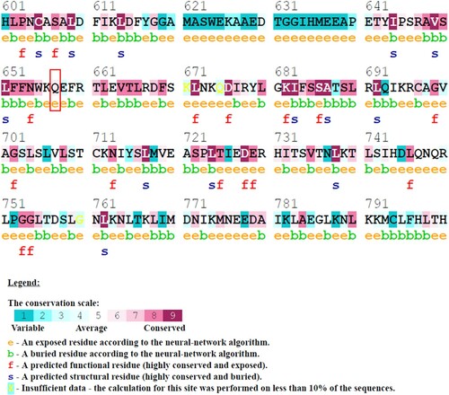
Table 1. Physicochemical properties of glutamine and leucine.

Characteristics	Glutamine	Leucine
Side chain flexibility	High	Moderate
Interaction modes	H-bonds, van der Waals	van der Waals
Potential side chain H-bonds	5	0
Residue molecular weight	128	113
Isoelectric point	5.7	6.0
Hydrophobicity	0.430	0.918
Standard codon(s)	CAR	CUN, UUR
Properties	Polar	Nonpolar
	Amide	Methylene
	Aliphatic	Aliphatic
	Non-essential	Essential

3.2. In silico pathogenicity prediction of Q657L mutation

The pathogenicity of the Q657L mutation was verified by six different prediction algorithms, namely Align-GVGD, SNAP2, SNPs&GO, SNPs3D, PON-P2, and PredictSNP. All prediction tools showed consistent results that the Q657L mutation is deleterious or disease-causing (Table 2); therefore, it may disrupt the protein structure and function.

Table 2. The pathogenicity prediction of Q657L mutation in NLRC4 using in silico prediction tools.

In silico prediction tools	Prediction score	Prediction
Align-GVGD	GV: 0.00; GD: 112.44	Class C65: Most likely to interfere with the function
SNAP2	37	Effect
SNPs&GO	0.667	Disease
SNPs3D	−1.69	Deleterious
PON-P2	0.810	Pathogenic
PredictSNP	–	Deleterious

3.3. Homology modelling and molecular dynamics simulation

The human full-length NLRC4 3D structure was modelled based on the human NLRC4 sequence (NCBI refseq ID: NP_001186067.1) and experimentally determined structures (PDB ID: 4KXF for resting conformation, PDB ID: 6B5B for activated conformation and PDB ID: 6N1I for CARD filament) using homology modelling. Both full-length NLRC4 models were of good quality as evaluated using PROCHECK, ERRAT and Verify3D. The wild-type NLRC4 protein in resting conformation was named RW, while the wild-type NLRC4 protein in the activated conformation was named AW. The mutated structures of the protein were prepared from these templates and named RM and AM, respectively. Then, all the models were subjected to MD simulation for 100 ns to investigate the effect of Q657L substitution on the structural and dynamic changes of the proteins.

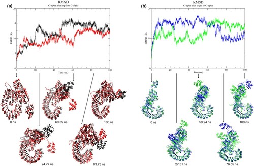
All systems (RW, RM, AW, and AM) had nearly invariant total energy throughout 100 ns simulation, ranging from −6.547 × 10⁶ kJ/mol to −2.693 × 10⁶ kJ/mol (Supporting Information Figure S3). This indicated that the simulations of these protein structures were stable and suitable for structural and dynamics analysis. Root-mean-square deviation (RMSD) of the Cα in each structure was determined to measure the variation between the Cα atom positions of a protein from its initial structure, which corresponds to the energy minimised structure. The RMSD plots showed that wild-type and mutant structures in resting and activated states deviated from their initial minimised structure throughout 100 ns MD simulations. For resting conformation, the wild-type structure showed a higher RMSD value compared to the mutant structure (RW structure: 0.005–16.743 Å; RM structure: 0.005–13.849 Å) (Figure 2(a)). A similar observation was seen in the activated conformation, where the wild-type structure showed a higher RMSD value than the mutant structure, particularly during the first 60 ns of simulation (AW structure: 0.005–17.578 Å; AM structure: 0.005–16.762 Å) (Figure 2(b)). The average values of RMSD for RW, RM, AW and AM were 12.05 ± 3.06 Å, 9.96 ± 2.10 Å, 13.44 ± 2.57 Å, and 12.04 ± 2.48 Å, respectively, throughout 100 ns MD simulation. As shown in Figure 2, during the first 65 ns of simulation for all structures (RW, RM, AW and AM), a large standard deviation of RMSD values was observed. Later, all structures achieved local equilibrium from 65 to 100 ns simulation with a smaller deviation. Therefore, the trajectories of 65–100 ns were used to analyse subsequent structural properties such as RMSF, secondary structures, Rg, SASA, and hydrogen bonding. To examine the conformational changes between wild-type and mutant structures, the snapshots at 0, 100 ns, and three selected snapshots with RMSD differences at three different time points were superimposed between RW and RM and between AW and AM (Figure 2). The observed differences in RMSD between mutant trajectories and wild-type trajectories would depict the overall conformational changes in the NLRC4 protein structure upon Q657L mutation.

Figure 2. (Colour online) Graph of RMSD values as a function of time and superposition of wild-type structure with the mutant structure. (a) Black denotes wild-type structure and red denotes mutant structure in the resting state. (b) Blue denotes wild-type structure and green denotes mutant structure in the activated state. The reference structures for the wild-type and mutant (at 0 ns) were the energy-minimised homology models. The simulations of all structures reached local equilibrium during 65–100 ns of simulation. The conformations of the mutant structures were different from the wild-type structures at a specific time point.

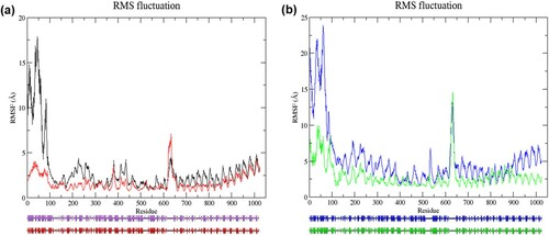
To understand how the dynamic behaviour of each amino acid residue was affected by the mutation, the root-mean-square fluctuation (RMSF) of Cα of each protein structure was calculated. RMSF is the square root of the variance of the atomic fluctuations around their average position. For resting confirmation, most of the residues in the mutant structure showed lower flexibility (RW structure: 0.826–17.898 Å; RM structure: 0.666–7.088 Å) (Figure 3(a)). In the activated state, the mutant structure also had lower flexibility in most of the residues (AW structure: 1.647–23.889 Å; AM structure: 1.156–14.573 Å) (Figure 3(b)). We observed that mutant structures (RM and AM) had lower average Cα-RMSF than their respective wild-type structures (RW and AW), in the last 35 ns of simulation. The average values of RMSF for RW, RM, AW and AM were 3.01 ± 2.78 Å, 1.69 ± 0.91 Å, 5.19 ± 3.86 Å, and 2.93 ± 1.78 Å, respectively. The high average Cα-RMSF in the wild-type structures was mainly due to higher flexibility in the N-terminal CARD, with a maximum value of 17.90 and 23.89 Å, respectively. When comparing the RMSF value of residue 657 in the mutant (RM and AM) structures with its wild-type counterparts (RW and AW), lower RMSF values were observed, such as 1.047 and 2.42 Å lesser, respectively. This finding is consistent with the result obtained from the amino acid explorer server, where the wild-type glutamine amino acid had higher side-chain flexibility (Table 1). Although the average Cα-RMSF values of wild-type structures were higher, a higher fluctuation at several residues in the LRR domain was observed in RM and AM structures, with a maximum value of 7.088 and 14.573 Å at residue 634 and residue 633, respectively. Structural analysis by PDBsum revealed secondary structural changes in the average structure of the mutant proteins in both states, particularly the region between residues 500–700 (Figure 3).

Figure 3. (Colour online) Graph of RMSF values of Cα atoms as a function of amino acids and predicted secondary structures of the average structures. (a) Cα atoms RMSF analysis of wild-type and mutant structure in the resting state (top). Black denotes wild-type structure and red denotes mutant structure in the resting state. Schematic wiring diagrams (bottom) show the secondary structure of the average structure (from 65 to 100 ns MD simulation). The purple diagram denotes wild-type average structure in the resting state; the red diagram denotes average mutant structure in the resting state. Strands are represented by arrows, and helices are represented by strings. (b) Cα atoms RMSF analysis of wild-type and mutant structure in the activated state (top). Blue denotes wild-type structure and green denotes mutant structure in the activated state. The schematic wiring diagram (bottom) in blue denotes wild-type average structure in the activated state, and green diagram denotes average mutant structure in the activated state. In both states, flexibility in mutant structure was lower than wild-type structure in most residues. In resting state, residues at locations, 143–145, 147, 149, 299, 330–331, 334, 336, 378–379, 520–521, 524–529, 535–537, 542, 545–546, 549, 553, 581, 590–596, 618–636, 643, 647–650, 873, 876–877, 905–907, 998–999, 1018–1020, were more flexible in mutant structure. The mutant structure exhibited higher fluctuation at residues 145, 412–414, 521, 530, 628–639, 771–775, 780, 798–812, 826–839, 855–868, 887–891 in the activated state. Schematic diagrams show changes in the secondary structures in the region between residues 3–30, 35–43, 61–75, 89–99, 193–194, 255–257, 281–286, 519–521, 648–654, 726–734, 795–802, 858–860, and 865–877 in the wild-type and mutant structure of the resting state. Changes of the secondary structures in the region between residues 65–84, 159–160, 251–262, 282–284, 288–290, 408–410,534–538, 602–608, 610–617, 795–801, 809–815, 859–860, and 888–889 were observed in the wild-type and mutant structure of the activated state.

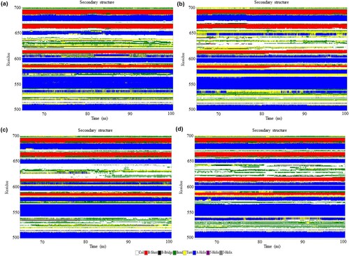
To understand the secondary structural changes in these four systems during 65–100 ns MD simulations, the secondary structure elements of each protein were assigned using the Database of Secondary Structure in Protein (DSSP) classification [45]. Considering high residual fluctuation and secondary structure change in the average structures between 500 and 700, the secondary structure change in this region was further inspected. There were conformational changes from helices, bend, and turn to bend, turn, and coil between the residues 524–525; helices to turn, bend, and helices between the residues 647–653 in the mutant structure of resting-state (Figure 4(a,b)). On the other hand, it is observed that conformational changes from helices, turn and bend to helices and turn forms between the residues 532 and 538; turn and helices to the coil, helices and bend forms between the residues 600 and 608; bend and coil to coil, bend, β-bridge and turn forms between the residues 611 and 617; coil and β-bridge to turn, bend, β-bridge and coil forms between the residues 641 and 645 in the mutant structure of the activated state (Figure 4(c,d)). These findings indicated that the Q657L mutation results in changes in the secondary structure in both states.

Figure 4. (Colour online) The secondary structure elements between the residues 500–700 of NLRC4 in the resting and activated state during 65–100 ns of simulation based on DSSP classification. (a) Wild-type structure in the resting state. (b) Mutant structure in the resting state. (c) Wild-type structure in the activated state. (d) Mutant structure in the activated state.

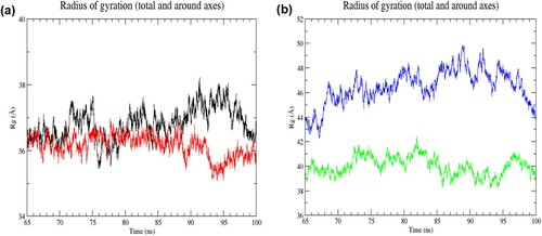
The radius of gyration (Rg) reflects the protein folding dynamics and compactness. Steady Rg values over the simulation denote the structure is stably folded, while lower Rg value indicates higher compactness. In the resting state, small variations in Rg values were observed in both structures over the simulation, indicating both structures were stably folded (Figure 5(a)). Moreover, the mutant structure attained slight lower Rg values than the wild-type structure (RW structure: 35.45–38.22 Å; RM structure: 35.08–36.98 Å), suggesting the mutant structure was more tightly packed than the wild-type structure. In the activated state, the mutant structure exhibited noticeably lower Rg values than the mutant structure (AW structure: 42.26–49.85 Å; AM structure: 38.16–42.41 Å) (Figure 5(b)), denoting a more compact packing of the mutant structure. The average value of Rg for RW, RM, AW, and AM was 36.81 ± 0.48 Å, 36.15 ± 0.33 Å 46.49 ± 1.37 Å and 40.01 ± 0.75 Å, respectively, in the last 35 ns of simulation. These findings suggested that the mutation affected protein compaction level, where the overall dimension of the protein was reduced. As shown in Figure 5, the Rg values of the structures in the activated state were higher than those in the resting state, indicating the expansion of protein structures in the activated state.

Figure 5. (Colour online) Radius of gyration (Rg) values of Cα atoms as a function of time from 65 to 100 ns of simulation. (a) Black denotes wild-type structure and red denotes mutant structure in the resting state. (b) Blue denotes wild-type structure and green denotes mutant structure in the activated state. The degree of compactness is reflected by the change in Rg value. A constant Rg value denotes no change in folding. In the resting state, the mutant structure was more stably folded than the wild-type structure in the last 35 ns of simulation. While the mutant structure was notably more compact than the wild-type structure in the activated state.

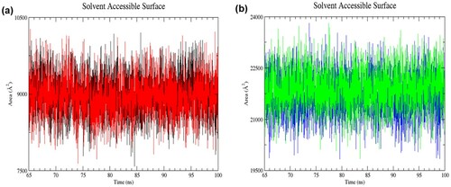
The solvent-accessible surface area (SASA) of each structure was calculated to evaluate the extent of surface area in contact with water molecules. A change in SASA value reflects changes in the tertiary structure. The SASA of the wild-type and mutant structures in the resting state was noticeably lower than those in the activated state during 65–100 ns of simulations (RW structure: 7584.9–10,195.9 Ų; RM structure: 7643.4–10,268.1 Ų; AW structure: 19,833.5–23,812.1 Ų; AM structure: 19,841.0–23,805.0 Ų) (Figure 6). This profile is consistent with the Rg analysis, indicating the expanded conformation of the activated structure allows more interactions of solvent with their hydrophobic core. The average SASA value of RW, RM, AW and AM was 8994.40 ± 382.37 Ų, 8955.42 ± 388.90 Ų, 21,711.10 ± 577.77 Ų and 21,890.64 ± 571.31 Ų, respectively, in the last 35 ns of simulation. It is observed that the average SASA value of the mutant structure in the activated state was higher than the wild-type structure, reflecting more solvent penetration into the core of the protein.

Figure 6. (Colour online) Solvent accessible surface area (SASA) of proteins as a function of time from 65 to 100 ns of simulation. (a) Black denotes wild-type structure and red denotes mutant structure in the resting state. (b) Blue denotes wild-type structure and green denotes mutant structure in the activated state. The wild-type and mutant structures in the activated state had higher SASA values than those in the resting state.

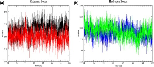
In addition, intramolecular and intermolecular hydrogen bonds were analysed in each structure to study the interactions between atoms in the protein and the interactions between the atoms of the protein with water molecules, respectively. Hydrogen bond interaction is required for maintaining protein stability, folding and function. In the resting state, the mutant structure had more intramolecular hydrogen bond formation than the wild-type structure in the last 35 ns of simulation (RW structure: 721–809; RM structure: 729–819) (Figure 7(a)). Contrarily, the number of intramolecular hydrogen bonds was decreased in the mutant structure of the activated state (AW structure: 699–787; AM structure: 688–783) (Figure 7(b)). The average number of intramolecular hydrogen bonds for RW, RM, AW and AM was 761 ± 12, 773 ± 12, 744 ± 12 and 735 ± 14, respectively, in the last 35 ns of simulation. As for the number of intermolecular hydrogen bonds formed, the wild-type structure had more numbers than the mutant structure in the resting state (RW structure: 2,144–2,320; RM structure: 2110–2299) (Figure 8(a)). Conversely, in the activated state, the mutant structure had more intermolecular hydrogen bonds (AW structure: 2184–2378; AM structure: 2180–2383) (Figure 8(b)). The average number of intermolecular hydrogen bonds for RW, RM, AW and AM was 2230 ± 25; 2198 ± 24; 2279 ± 27 and 2285 ± 29, respectively, in the last 35 ns of simulation. Changes in the intermolecular hydrogen bonding may affect protein conformation, folding specificity, stability, and dynamics.

Figure 7. (Colour online) The number of intramolecular hydrogen bonds as a function of time from 65 to 100 ns of simulation. (a) Black denotes wild-type structure and red denotes mutant structure in the resting state. (b) Blue denotes wild-type structure and green denotes mutant structure in the activated state. In the resting state, more numbers of intramolecular bonds were formed in the mutant than in the wild-type structure. The mutant structure had lesser intramolecular hydrogen bonds than the wild-type structure in the activated state.

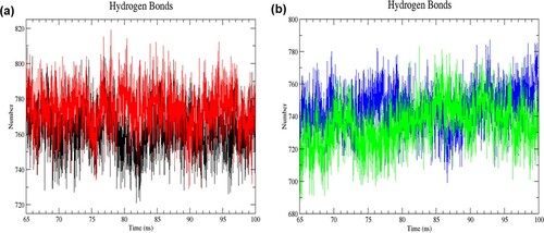
Figure 8. (Colour online) The number of intermolecular hydrogen bonds as a function of time from 65 to 100 ns of simulation. (a) Black denotes wild-type structure and red denotes mutant structure in the resting state. (b) Blue denotes wild-type structure and green denotes mutant structure in the activated state. Lesser intermolecular bonds were formed in the mutant than the wild-type structure in the resting state. The mutant structure had more intermolecular hydrogen bonds than the wild-type structure in the activated state.

3.4. Essential dynamics and Gibbs free energy landscape

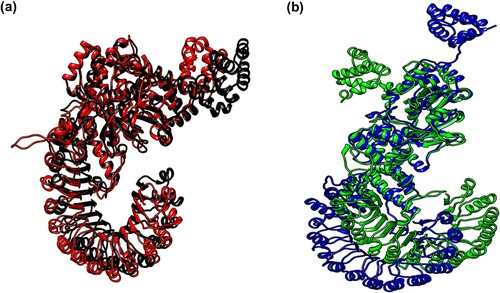
The biological function of a protein is determined by its well-defined conformation and dynamics. To examine the overall motions of the wild-type and mutant structures, principal component analysis (PCA) was carried out. It is noted that the trace of the diagonalised covariance matrix of Cα atomic positional fluctuations for the mutant structure was smaller than the wild-type structure in both states (RW structure: 17,209.60 Ų; RM structure: 3790.21 Ų; AW structure: 42,901.90 Ų; AM structure: 12,007.90 Ų), demonstrating the mutant structures had decreased overall motions compared to its counterpart. The eigenvalues of the wild-type and mutant structures in both states were plotted against their corresponding eigenvector index for the first ten modes of motion (Figure 9(a,b)). The result showed that the first two eigenvectors had noticeably higher eigenvalues, indicating most of the internal motions of the wild-type and mutant structures in both states were confined to these two eigenvectors. To inspect the patterns of overall motions in the wild-type and mutant structures, all trajectories of 65–100 ns simulation were projected onto a 2D essential subspace represented by the first two principal components (PC1 and PC2) (Figure 9(c,d)). In the resting state, the wild-type structure displayed the scattered type of motions, occupying space on PC1 (between −231 and 178 Å) and PC2 (between −132 and 114 Å) (Figure 9(c)). In contrast, the mutant structure exhibited cluster type motions, covering a smaller space on PC1 (between −91 and 69 Å) and PC2 (between −77 and 89 Å), respectively. In the activated state, a similar observation was noted where the wild-type structure had more dispersed motions and covered more space on PC1 (between −272 and 306 Å) and PC2 (between −245 and 217 Å) (Figure 9(d)). Meanwhile, the overall motions of the mutant structure were restrained on PC1 (between −156 and 127 Å) and PC2 (between −123 and 130 Å). These findings demonstrated decreased overall flexibility of mutant structures in both states. Furthermore, it is observed that the value for subspace overlaps of the mutant structure against the wild-type structure was 17.5% and 23.5%, in the resting and activated state, respectively. Gibbs free energy landscape (FEL) plot was generated using the first two principal components (PC1 and PC2). The initial Gibbs free energy of wild-type and mutant structures in the resting and activated state ranged from 9.26 to 9.88 kJ/mol (Figure 10). Cluster analysis showed that the representative structures of wild-type and mutant proteins obtained from their top cluster were dissimilar in both states (Figure 11). These findings indicated a low degree of similarity in the conformational freedom between these two structures, reflecting dynamics and functional differences between the wild-type and mutant structures in both states.

Figure 9. (Colour online) Principal component analysis of NLRC4 during the last 35 ns of simulation. (a) The plot of eigenvalues vs. eigenvector index for the first ten eigenvectors of wild-type and mutant structure in the resting state. Black denotes wild-type structure and red denotes mutant structure in the resting state. (b) Plot of eigenvalues vs. eigenvector index for the first ten eigenvectors of wild-type and mutant structure in the activated state. Blue denotes wild-type structure and green denotes mutant structure in the activated state. (c) 2D projection of the motion for wild-type and mutant structure in resting state. (d) 2D projection of the motion for wild-type and mutant structure in the activated state. In both states, both mutant structures (RM and AM) occupied a smaller region of phase space than the wild-type structures (RW and AW), indicating a decrease in the overall flexibility of mutant structures in the last 35 ns of simulations.

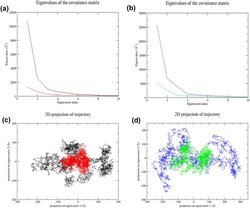
Figure 10. (Colour online) Gibbs free energy landscapes of the first two principal components (PC1 and PC2) during 65–100 ns MD simulation. The free energy value is given in kJ/mol shown by the colour bar. The blue colour region in the plot indicates lower energy. (a) Wild-type structure in the resting state. (b) Mutant structure in the resting state. (c) Wild-type structure in the activated state. (d) Mutant structure in the activated state.

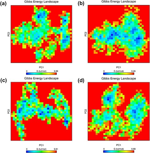
Figure 11. (Colour online) Cluster analysis of MD simulation trajectories of NLRC4 proteins. The representative structure of the top cluster obtained from the trajectories of 65–100 ns MD simulation. (a) Superposition of the representative structure of wild-type (black) and mutant (red) protein in the resting state. (b) Superposition of the representative structure of wild-type (blue) and mutant (green) protein in the activated state.

3.5. Binding pocket volume

There was no prominent change in the binding pocket volume of wild-type and mutant structures in the resting state (RW structure: 7815.98 ų; RM structure: 7946.527 ų). While a remarkable increase in binding pocket volume was observed for the mutant structure of the activated state (AW structure: 3448.448 ų; AM structure: 14,289.293 ų), reflecting an increased chance of binding to other molecules.

4. Discussion

Inflammation is a body defence mechanism against hazardous stimuli, such as cellular damage, pathogenic microorganisms, irradiation or toxic compounds [46]. In contrast, auto-inflammation is characterised by an aberrant innate immune response that leads to systemic or organ-specific inflammation in the absence of infection, malignancy or antigen-specific autoimmunity [47]. Autoinflammatory disorders can be induced by genetic mutations in genes encoding a protein involved in the pathways of the inflammasome, such as NLRC4 protein [48]. In our previous study, we identified a novel de novo NLRC4 mutation (Q657L) in the LRR domain associated with the autoinflammatory disorder. Increased levels of downstream pro-inflammatory cytokines observed in the patient maybe due to spontaneous inflammasome activation caused by Q657L mutation [13]. However, the exact molecular mechanism behind Q657L mutation causing spontaneous inflammasome activation remains unknown. Therefore, our current study aimed to investigate the functional role of conserved residue at position 657 of NLRC4 protein and its association with autoinflammatory disorder.

The physicochemical properties of glutamine and leucine residues differed in terms of the residue size, charge, hydrophobicity, side-chain flexibility, potential side-chain hydrogen bond, and isoelectric point. The glutamine residue at position 657 in NLRC4 was predicted as a conserved and exposed amino acid by the ConSurf server. Moreover, the Q657L mutation was predicted as pathogenic by various in silico prediction tools. Therefore, the substitution of glutamine for leucine amino acid might alter the biological function of NLRC4 protein. In the present study, a homology-based method was used to construct full-length 3D structures of human monomeric NLRC4 in the resting and activated state using experimentally determined structures (PDB ID: 4KXF; 6B5B; 6N1I). The mouse 3D structures were used as the templates as they shared 70% sequence identity with the human NLRC4 sequence. Subsequently, computational mutagenesis was performed to generate the Q657L mutant structures. High-quality homology models were used as the starting structures for molecular dynamics (MD) simulation, which captured the dynamic behaviour of a protein at an atomic level over time [49].

The reliability of a molecular dynamics simulation depends on the accuracy of the underlying force field and water model. In the study of protein structure molecular dynamics simulation, the CHARMM36 all-atom additive protein force field has shown a better correlation with experimental data than other force fields [50]. The CHARMM36 force field was parameterised to rebalance the equilibrium between the sampling of helical and extended conformations. However, the use of CHARMM36 in a combination of the mTIP3P water model was shown to increase solvation to the peptide leading to a suppression of peptide folding [51]. Recently, an improved force field, CHARMM36m, has been optimised to overcome the protein-water interactions and validated parameters for proteins [36]. The use of CHARMM36m force field along with a modified TIP3P water model has been shown to accurately model a targeted protein and enhance sampling of conformational space, but the issue of over compactness in protein might be a potential impact [52]. In this study, CHARMM36m, with a modified TIP3P water model, was used for MD simulations.

The NLRC4 protein exists as a monomer in the resting state [5]. Upon activation, ADP hydrolysis results in NLRC4 conformational change prerequisite for oligomerisation and inflammasome activation [47]. It has been demonstrated that the binding interfaces for partner proteins are pre-formed in the monomeric protein [53]. Furthermore, the conformations of the binding interfaces on the unbound protein were similar to those in the bound state [54]. Therefore, monomeric wild-type and mutant structures in both resting state and activated state were subjected to MD simulation in the absence of a binding partner to investigate the structural and dynamics impact of the Q657L mutation. The RMSD analysis is used to evaluate the degree of structural similarity between two structures, as well as the extent of equilibration of the simulation [17,55]. The superposition of wild-type and mutant structures at several time points illustrated structural differences between these structures. This was further corroborated by changes in the hydrogen bonds and secondary structures, as evident by hydrogen bond and DSSP analysis. Based on RMSD analysis, all structures achieved local equilibrium in the last 35 ns of simulation. Therefore, the trajectories from 65 to 100 ns MD simulation were used to analyse other structural and dynamics parameters.

In the resting state, the RMSF analysis showed that the ADP-unbound mutant structure attained lower average Cα-RMSF values, indicating that the mutant structure was less flexible than the wild-type structure. Structural flexibility and conformational adjustment to the binding partners may regulate binding processes [56]. ADP is critical for securing NLRC4 structure in autoinhibited conformation. Residues P119, F128, T135, G174, G172, K175, S176, T177, P338 and H443 are involved in the ADP binding [5]. Structural flexibility enables the protein to accommodate their molecular binding partners and aid in the binding process [56]. Increased local flexibility may enhance substrate-binding affinity [57,58]. Lower flexibility observed in these residues of the mutant structure might affect the substrate binding interface mobility, which is crucial for the ADP binding process.

As a result, the ADP binding ability might be affected and subsequently disrupt the autoinhibitory mechanism in the resting state. However, high flexibility was noted in the residues (D143-H145, H147, V149, and D299 in NBD; G520, L521, A524-W529, Q535-V537, E542, I545-L546, I549, and S553 in HD2) which mainly constituted the loop regions. G520 residue is an important residue in the HD2 which acts as a supporting point for the packing of NLRC4 [5]. High flexibility in these residues may lead to mobility of NBD and HD2, which may affect the accessibility of ADP molecule to the binding site, and hence distort the conformation required for maintaining autoinhibition. Moreover, the Rg analysis showed that the mutant structure attained lower Rg values, revealing that the structure was more rigid. This rigid structure was further supported by an increased number of intramolecular hydrogen bonds. Additionally, principal component analysis (PCA) clearly showed that the mutant structure had decreased overall flexibility compared to the wild-type structure. Changes in protein dynamics often reflect a change in molecular structure or conformation over time, associated with biological function [59]. In other words, the wild-type structure attained a more open and relaxed conformation than the mutant structure, as shown by RMSF, Rg, hydrogen bonding analysis and PCA, which may facilitate ADP binding process and achieve an autoinhibitory state.

In the activated state, the mutant structure attained a higher solvent accessible surface area (SASA) value and binding pocket volume than the wild-type structure. The SASA value reflects the surface area of a protein accessible by solvent molecules [60]. The protein surface is well distributed with binding interfaces filled with water molecules during its unbound state. Some of these water molecules reside permanently in the binding interface, maintaining interface flexibility [53]. Conversely, some water molecules are readily displaced by the atoms of the binding partners, which favour association [61]. An increase in the SASA values may indicate an increased overall molecular surface that can interact with solvent, which may reflect more interfaces that can interact with atoms on the surface of the partner protein [62]. The strength of oligomeric interaction is determined by the nature of the oligomer interface and the duration of the interaction. For instance, large oligomeric interfaces are associated with strong interactions. Increased intermolecular hydrogen bonds were observed in the mutant structure, contributing to the stability and specificity of oligomeric interactions between oligomers [63]. Contrarily, the mutant structure had lesser intramolecular hydrogen bonds. It has been found that increased SASA values may be associated with the decreased frequency of intramolecular hydrogen bonds formed [64], which was consistent with our finding. Changes in the number of hydrogen bonds might affect the folding pattern, the structural integrity and thus the protein’s function [64–66].

Oligomerisation might be determined by the folding of individual oligomers [67], where a more compact oligomer is preferable for self-association [68]. The Rg analysis demonstrated that the mutant structure was more stably folded into a more compact structure than the wild-type structure in the activated state. Moreover, the mutant structure had lower overall flexibility, as shown by PCA. These findings suggested that the activated mutant structure may appear as a more favourable oligomer for self-assembly. For self-assembly, it has been demonstrated that the NBD and LRR domain of NLRC4 protein is involved in the formation of inflammasome complex [6]. The RMSF analysis demonstrated higher flexibility was observed in some residues (H145 of NBD; A628-A639, D771-M775, A780, L798-V812, Q826-I839, L855-E868, P887-D891 of LRR domain) in the mutant structure. The increased local flexibility at these sites may affect the ability of NLRC4 to interact with other partner proteins.

5. Conclusion

In the present study, the pathogenicity of the Q657L mutation was assessed and characterised using computational prediction approaches. The Q657L mutation was predicted to be deleterious and disease-causing by various in silico prediction tools. MD simulations were performed to investigate conformational and dynamics changes using the homology-modelled full-length human NLRC4 wild-type and mutant structures in the resting and activated state. The MD simulation results demonstrated that the mutant structure changed compactness, flexibility, and hydrogen bond interactions in the resting state. On the other hand, increased compactness, solvent accessible surface area, intermolecular hydrogen bonds and binding pocket volume were observed in the mutant structure, rendering it to be appeared as a favourable conformation required for oligomerization. Our results show how a point mutation in the protein-coding sequence may lead to a severe change in the protein structure and subsequently affects its function. Understanding the impacts of NLRC4 mutation on protein structure and function provides insights into the molecular mechanism associated with disease and facilitates novel drug discovery.

Acknowledgements

We would like to thank the Director General of Health Malaysia for his permission to publish this article. The homology modelling and MD simulations in this work were supported by the Centre of Research in Systems Biology, Structural Bioinformatics and Human Digital Imaging (CRYSTAL), Universiti Malaya. We also gratefully acknowledge Ridzwan FW for the technical assistance.

Disclosure statement

No potential conflict of interest was reported by the author(s).

Additional information

Funding

This work was supported by the Ministry of Health, Malaysia (NMRR-16-892-31023).

References

- Krainer J, Siebenhandl S, Weinhäusel A. Systemic autoinflammatory diseases. J Autoimmun. 2020;109:102421.
- Tangye SG, Al-Herz W, Bousfiha A, et al. Human inborn errors of immunity: 2019 update on the classification from the international union of immunological societies expert committee. J Clin Immunol. 2020;40:24–64.
- Manthiram K, Zhou Q, Aksentijevich I, et al. The monogenic autoinflammatory diseases define new pathways in human innate immunity and inflammation. Nat Immunol. 2017;18:832–842.
- Fusco WG, Duncan JA. Novel aspects of the assembly and activation of inflammasomes with focus on the NLRC4 inflammasome. Int Immunol. 2018;30:183–193.
- Hu Z, Yan C, Liu P, et al. Crystal structure of NLRC4 reveals its autoinhibition mechanism. Science. 2013;341:172–175.
- Zhang L, Chen S, Ruan J, et al. Cryo-EM structure of the activated NAIP2-NLRC4 inflammasome reveals nucleated polymerization. Science. 2015;350:404–409.
- Weiss ES, Girard-Guyonvarc’h C, Holzinger D, et al. Interleukin-18 diagnostically distinguishes and pathogenically promotes human and murine macrophage activation syndrome. Blood. 2018;131:1442–1455.
- Romberg N, Moussawi KA, Nelson-Williams C, et al. Mutation of NLRC4 causes a syndrome of enterocolitis and autoinflammation. Nat Genet. 2014;46:1135–1139.
- Canna SW, Jesus AAD, Gouni S, et al. An activating NLRC4 inflammasome mutation causes autoinflammation with recurrent macrophage activation syndrome. Nat Genet. 2014;46:1140–1146.
- Kitamura A, Sasaki Y, Abe T, et al. An inherited mutation in NLRC4 causes autoinflammation in human and mice. J Exp Med. 2014;211:2385–2396.
- Kawasaki Y, Oda H, Ito J, et al. Identification of a high-frequency somatic NLRC4 mutation as a cause of autoinflammation by pluripotent cell-based phenotype dissection. Arthr Rheumatol. 2017;69:447–459.
- Moghaddas F, Zeng P, Zhang Y, et al. Autoinflammatory mutation in NLRC4 reveals a leucine-rich repeat (LRR)–LRR oligomerization interface. J Allergy Clin Immunol. 2018;142:1956–1967.
- Chear CT, Nallusamy R, Canna SW, et al. A novel de novo NLRC4 mutation reinforces the likely pathogenicity of specific LRR domain mutation. Clin Immunol. 2020;211:108328.
- Volker-Touw CML, de Koning HD, Giltay JC, et al. Erythematous nodes, urticarial rash and arthralgias in a large pedigree with NLRC4-related autoinflammatory disease, expansion of the phenotype. Br J Dermatol. 2017;176:244–248.
- Liang J, Alfano DN, Squires JE, et al. Novel NLRC4 mutation causes a syndrome of perinatal autoinflammation with hemophagocytic lymphohistiocytosis, hepatosplenomegaly, fetal thrombotic vasculopathy, and congenital anemia and ascites. Pediatr Dev Pathol. 2017;20:498–505.
- Jeskey J, Parida A, Graven K, et al. Novel gene deletion in NLRC4 expanding the familial cold inflammatory syndrome phenotype. Allergy Rhinol. 2020;11:215265672092806.
- Kumar R, Bansal A, Shukla R, et al. In silico screening of deleterious single nucleotide polymorphisms (SNPs) and molecular dynamics simulation of disease associated mutations in gene responsible for oculocutaneous albinism type 6 (OCA 6) disorder. J Biomol Struct Dyn. 2019;37:3513–3523.
- Panchal NK, Bhale A, Verma VK, et al. Computational and molecular dynamics simulation approach to analyze the impact of XPD gene mutation on protein stability and function. Mol Simulat. 2020;46:1200–1219.
- Essadssi S, Krami AM, Elkhattabi L, et al. Computational analysis of nsSNPs of ADA gene in severe combined immunodeficiency using molecular modeling and dynamics simulation. J Immunol Res. 2019;2019:1–14.
- Venselaar H, te Beek TA, Kuipers RK, et al. Protein structure analysis of mutations causing inheritable diseases. An e-Science approach with life scientist friendly interfaces. BMC Bioinform. 2010;11:548.
- Mayrose I. Comparison of site-specific rate-inference methods for protein sequences: Empirical Bayesian methods are superior. Mol Biol Evol. 2004;21:1781–1791.
- Ashkenazy H, Erez E, Martz E, et al. Consurf 2010: calculating evolutionary conservation in sequence and structure of proteins and nucleic acids. Nucl Acid Res. 2010;38:W529–W533.
- Celniker G, Nimrod G, Ashkenazy H, et al. Consurf: using evolutionary data to raise testable hypotheses about protein function. Isr J Chem. 2013;53:199–206.
- Ashkenazy H, Abadi S, Martz E, et al. Consurf 2016: an improved methodology to estimate and visualize evolutionary conservation in macromolecules. Nucl Acid Res. 2016;44:W344–W350.
- Tavtigian SV. Comprehensive statistical study of 452 BRCA1 missense substitutions with classification of eight recurrent substitutions as neutral. J Med Genet. 2005;43:295–305.
- Hecht M, Bromberg Y, Rost B. Better prediction of functional effects for sequence variants. BMC Genom. 2015;16:S1.
- Calabrese R, Capriotti E, Fariselli P, et al. Functional annotations improve the predictive score of human disease-related mutations in proteins. Hum Mutat. 2009;30:1237–1244.
- Yue P, Melamud E, Moult J. SNPs3d: Candidate gene and SNP selection for association studies. BMC Bioinform. 2006;7:166.
- Niroula A, Urolagin S. Vihinen M. PON-P2: prediction method for fast and reliable identification of harmful variants. Tosatto SCE, editor. PLoS One. 2015;10:e0117380.
- Bendl J, Stourac J, Salanda O, et al. PredictSNP: robust and accurate consensus classifier for prediction of disease-related mutations. Gardner PP, editor. PLoS Comput Biol. 2014;10:e1003440.
- Laskowski RA, MacArthur MW, Moss DS, et al. PROCHECK: a program to check the stereochemical quality of protein structures. J Appl Crystallogr. 1993;26:283–291.
- Bowie JU, Luthy R, Eisenberg D. A method to identify protein sequences that fold into a known three-dimensional structure. Science. 1991;253:164–170.
- Colovos C, Yeates TO. Verification of protein structures: patterns of nonbonded atomic interactions. Protein Sci. 1993;2:1511–1519.
- Spoel DVD, Lindahl E, Hess B, et al. GROMACS: fast, flexible, and free. J Comput Chem. 2005;26:1701–1718.
- Abraham MJ, Murtola T, Schulz R, et al. GROMACS: high performance molecular simulations through multi-level parallelism from laptops to supercomputers. SoftwareX. 2015;1–2:19–25.
- Huang J, Rauscher S, Nawrocki G, et al. CHARMM36m: an improved force field for folded and intrinsically disordered proteins. Nat Methods. 2017;14:71–73.
- Bussi G, Donadio D, Parrinello M. Canonical sampling through velocity rescaling. J Chem Phys. 2007;126:014101.
- Berendsen HJC, Postma JPM, van Gunsteren WF, et al. Molecular dynamics with coupling to an external bath. J Chem Phys. 1984;81:3684–3690.
- Hess B, Kutzner C, van der Spoel D, et al. GROMACS 4: algorithms for highly efficient, load-balanced, and scalable molecular simulation. J Chem Theory Comput. 2008;4:435–447.
- Darden T, York D, Pedersen L. Particle mesh Ewald: An N ⋅log(N) method for Ewald sums in large systems. J Chem Phys. 1993;98:10089–10092.
- Laskowski RA. PDBsum new things. Nucl Acid Res. 2009;37:D355–D359.
- Daura X, van Gunsteren WF, Mark AE. Folding-unfolding thermodynamics of a β-heptapeptide from equilibrium simulations. Proteins. 1999;34:269–280.
- Amadei A, Linssen ABM, Berendsen HJC. Essential dynamics of proteins. Proteins. 1993;17:412–425.
- Tian W, Chen C, Lei X, et al. CASTp 3.0: computed atlas of surface topography of proteins. Nucl Acid Res. 2018;46:W363–W367.
- Kabsch W, Sander C. Dictionary of protein secondary structure: pattern recognition of hydrogen-bonded and geometrical features. Biopolymers. 1983;22:2577–2637.
- Chen L, Deng H, Cui H, et al. Inflammatory responses and inflammation-associated diseases in organs. Oncotarget. 2018;9:7204–7218.
- Duncan JA, Canna SW. The NLRC4 inflammasome. Immunol Rev. 2018;281:115–123.
- Schnappauf O, Aksentijevich I. Current and future advances in genetic testing in systemic autoinflammatory diseases. Rheumatology. 2019;58:vi44–vi55.
- Hollingsworth SA, Dror RO. Molecular dynamics simulation for all. Neuron. 2018;99:1129–1143.
- Huang J, MacKerell AD. CHARMM36 all-atom additive protein force field: validation based on comparison to NMR data. J Comput Chem. 2013;34:2135–2145.
- Boonstra S, Onck PR, van der Giessen E. CHARMM TIP3P water model suppresses peptide folding by solvating the unfolded state. J Phys Chem B. 2016;120:3692–3698.
- Pineda LI G, Milko LN, He Y. Performance of CHARMM36m with modified water model in simulating intrinsically disordered proteins: a case study. Biophys Rep. 2020;6:80–87.
- Li X, Keskin O, Ma B, et al. Protein–protein interactions: Hot spots and structurally conserved residues often locate in complemented pockets that pre-organized in the unbound states: implications for docking. J Mol Biol. 2004;344:781–795.
- Rajamani D, Thiel S, Vajda S, et al. Anchor residues in protein-protein interactions. Proc Nat Acad Sci. 2004;101:11287–11292.
- George DCP, Chakraborty C, Haneef SS, et al. Evolution- and structure-based computational strategy reveals the impact of deleterious missense mutations on MODY 2 (maturity-onset diabetes of the young, type 2). Theranostics. 2014;4:366–385.
- Stank A, Kokh DB, Fuller JC, et al. Protein binding pocket dynamics. Acc Chem Res. 2016;49:809–815.
- Garton M, MacKinnon SS, Malevanets A, et al. Interplay of self-association and conformational flexibility in regulating protein function. Phil Trans R Soc B. 2018;373:20170190.
- Marcos E, Crehuet R, Bahar I. Changes in dynamics upon oligomerization regulate substrate binding and allostery in amino acid kinase family members. Gilson M, editor. PLoS Comput Biol. 2011;7:e1002201.
- Yang LQ, Sang P, Tao Y, et al. Protein dynamics and motions in relation to their functions: several case studies and the underlying mechanisms. J Biomol Struct Dyn. 2014;32:372–393.
- Eisenhaber F, Lijnzaad P, Argos P, et al. The double cubic lattice method: efficient approaches to numerical integration of surface area and volume and to dot surface contouring of molecular assemblies. J Comput Chem. 1995;16:273–284.
- Janin J, Bahadur RP, Chakrabarti P. Protein–protein interaction and quaternary structure. Quart Rev Biophys. 2008;41:133–180.
- Keskin O, Gursoy A, Ma B, et al. Principles of protein–protein interactions: what are the preferred ways for proteins to interact? Chem Rev. 2008;108:1225–1244.
- Ali MH, Imperiali B. Protein oligomerization: How and why. Bioorgan Med Chem. 2005;13:5013–5020.
- Efimov AV, Brazhnikov EV. Relationship between intramolecular hydrogen bonding and solvent accessibility of side-chain donors and acceptors in proteins. FEBS Lett. 2003;554:389–393.
- Hubbard RE, Haider MK. Hydrogen bonds in proteins: role and strength. eLS. 2010:1–7.
- Pace CN, Fu H, Fryar K, et al. Contribution of hydrogen bonds to protein stability: hydrogen bonds and protein stability. Protein Sci. 2014;23:652–661.
- Lesieur C. The assembly of protein oligomers: old stories and new perspectives with graph theory. Oligomeriz Chem Biol Compound. 2014:327–364.
- Tsai C-J, Xu D, Nussinov R. Protein folding via binding and vice versa. Fold Des. 1998;3:R71–R80.