Degrees of freedom of atoms in a rigid molecule for local temperature calculation in molecular dynamics simulation

ABSTRACT

In molecular dynamics simulation, it is quite common to calculate a precise temperature profile with an atomic or sub-angstrom resolution. While this calculation typically requires the degrees of freedom (DOF) of individual atoms, those in a molecule subject to geometric constraints is undefined in general. Conventionally, the approximation of subtracting from the atom DOF by 1/2 per one distance constraint has been used, but this approximation is valid for spatially homogeneous systems only. In the present study, on the basis of statistical mechanics, we derived more general expressions for the DOF of atoms in fully or partially rigid molecules. The expressions ensure that in an equilibrium state, all constrained atoms have the same temperature as the equilibrium temperature of the whole system and are also applicable to inhomogeneous systems.

KEYWORDS:

• Molecular dynamics
• mechanical degrees of freedom
• local temperature
• rigid molecule
• constraint
• linked rigid body

1. Introduction

In molecular dynamics (MD) simulations [1], it is quite common to calculate temperature profiles, i.e. the spatial distribution of local temperature. Such temperature profiles are not only the theoretical predictions of temperature distributions in real materials and phenomena [2,3], but also utilised in various ways. In non-equilibrium MD simulations of heat conduction, the gradient and jump in temperature profiles are used to derive thermodynamic coefficients [4] and thermal transport properties [5,6]. Temperature difference among different atoms or vibrational modes can be examined to check if the system is thermally equilibrated [7,8]. The local temperature fields computed with MD simulations provide reference data in developing more coarse-grained computational fluid dynamic schemes [9,10]. These applications typically require a precise temperature profile with an atomic or sub-angstrom resolution.

On the other hand, MD systems may be subject to geometric constraints in order to allow for a larger simulation timestep and to suppress vibration modes that should not be excited in view of quantum mechanics [11]. In particular, freezing bond lengths and angles involving fast vibrations of hydrogen atoms is often useful [12]. Such constraints are achieved either by imposing holonomic constraints in the equation of motion for a point mass [11,13], or by modelling a molecule or part of a molecule as a rigid body and solving Euler’s equation of motion for a rigid body [14]. There is a problem when one calculates temperature profiles in a system subject to such constraints. A single constrained molecule usually spans multiple local volumes used for the local temperature calculation. In this case, the total degrees of freedom (DOF) in a local volume must be obtained by summing up the DOF of individual atoms. However, while the DOF per free atom is known to be 3 (in the 3-dimensional space), the DOF of atoms in a geometrically constrained molecule is undefined in general. For the constraint of the distance between two atoms, a convenient approximation is that each of the two atoms has the DOF reduced by 1/2 [12]. This even-distribution approximation is reasonable when the two atoms are contained in a local volume with similar probabilities or are of the same atom type, and it has been appropriately applied to spatially uniform liquids [12,15,16]. On the contrary, the atom DOF should be determined more carefully in systems where the distribution of the constituent atoms is highly inhomogeneous, such as nanostructures and interfaces of different phases. However, to our knowledge, explicit DOF expressions for constrained atoms in such inhomogeneous systems has not been discussed yet. In the present study, we derive them based on statistical mechanics, together with the validation by MD simulations. The specific expression depends on how the molecular geometry is constrained. Here, we particularly focus on the DOF of atoms in (i) a rigid molecule and (ii) a three-atom molecule with two distance constraints but no angle constraint. These examples cover many of the constrained systems dealt with in current MD research.

2. Expressions for the DOF of constrained atoms

2.1. Definition

The temperature T_loc of a local volume V_loc is most commonly calculated via the kinetic temperature definition: (1) $〈\sum _{i\in V_{\mathrm{l}\mathrm{o}\mathrm{c}}}{K}_i〉=\sum _{i\in V_{\mathrm{l}\mathrm{o}\mathrm{c}}}{\displaystyle \frac{1}{2}{g}_i{k}_{\mathrm{B}}{T}_{\mathrm{l}\mathrm{o}\mathrm{c}}},$(1) where g_i, K_i = m_iv_i²/2, m_i, and v_i are the DOF, kinetic energy, mass, and velocity vector of atom i, respectively, k_B is the Boltzmann constant, and 〈 … 〉 denotes the ensemble average. Similarly, the temperature of atom i is defined by (2) $〈K_i〉={\displaystyle \frac{1}{2}{g}_i{k}_{\mathrm{B}}{T}_i}$(2)

In the even-distribution approximation, which is conventionally used, g_i for constrained atoms is described as (3) $g_i=3\text{–}{n}_{c,i}/2,$(3) where n_c,i is the number of distance constraints that involve atom i. Although this approximation is quite convenient, its use is restricted to homogeneous systems.

To derive an atom DOF that is applicable in general cases, we begin with the following definition: (4) $g_i=2{〈K_i〉}_T/\left(k_{\mathrm{B}}T\right)$(4) where 〈K_i〉_T is the average kinetic energy of atom i evaluated in an equilibrium state at a temperature T. Although Equation (2) and Equation (4) similar in appearance, their physical meanings are completely different: Equation (2) is the definition of atom temperature when the value of g_i is known. In contrast, Equation (4) is the definition of g_i based on a reasonable requirement that at least in an equilibrium state, the temperature of a constrained atom calculated by Equation (2) is equal to the equilibrium temperature. The atom kinetic energy in Equation (4) can be evaluated in any equilibrium state. Here, for simplicity, we assume a canonical ensemble. For an N atom system, the atom kinetic energy is expressed as (5) $\begin{array}{rl}& {〈K_i〉}_T\\ & ={\displaystyle \frac{{\int }_{}^{}1/2m_i{\mathit{v}}_i^2{e}^{-H({\mathit{r}}_1,\dots ,{\mathit{r}}_N,{\mathit{v}}_1,\dots ,{\mathit{v}}_N)/k_{\mathrm{B}}T}{f}_{\mathrm{c}\mathrm{n}\mathrm{s}}\left(\mathit{\gamma }\right)d{\mathit{r}}_1\cdots d{\mathit{r}}_{N}d{\mathit{v}}_1\cdots d{\mathit{v}}_N}{{\int }_{}^{}{e}^{-H({\mathit{r}}_1,\dots ,{\mathit{r}}_N,{\mathit{v}}_1,\dots ,{\mathit{v}}_N)/k_{\mathrm{B}}T}{f}_{\mathrm{c}\mathrm{n}\mathrm{s}}\left(\mathit{\gamma }\right)d{\mathit{r}}_1\cdots d{\mathit{r}}_{N}d{\mathit{v}}_1\cdots d{\mathit{v}}_N},}\end{array}$(5) where $H({\mathit{r}}_1,\dots ,{\mathit{r}}_N,{\mathit{v}}_1,\dots ,{\mathit{v}}_N)$ is the Hamiltonian of the system, i.e. the sum of the kinetic and potential energies, described here as a function of the coordinate vector r_i and velocity vector v_i of atom i. The function f_cns(γ) is necessary to take geometric constraints into account and γ represents the set of coordinates and velocities that are relevant to the constraints. For example, suppose that the distance between atoms i and j is constrained to a constant value d as r_ij = |r_i – r_j| = d and this is the only geometrical constraint in the system. The atom velocities are also constrained since the time derivative of r_ij must be zero as $d{r}_{ij}/dt\equiv {\dot{r}}_{ij}=0$. This constraint is expressed as $f_{\mathrm{c}\mathrm{n}\mathrm{s}}(r_{ij},{\dot{r}}_{ij})=\delta (r_{ij}-d)\delta \left({\dot{r}}_{ij}\right)$, where δ is the Dirac delta function. Since $f_{\mathrm{c}\mathrm{n}\mathrm{s}}(r_{ij},{\dot{r}}_{ij})$ depends on r_i, r_j, v_i, and v_j, this function implicitly makes v_i dependent of r_i, r_j, and v_j. In the general case, f_cns is defined in a similar way. Then, with an appropriate transformation of integral variables, γ and other variables irrelevant to K_i can be integrated out, and the result is formally written as (6) ${〈K_i〉}_T={\int }_{}^{}{\displaystyle \frac{1}{2}{m}_i{\mathit{v}}_i^2{e}^{-H_{\mathrm{p}\mathrm{a}\mathrm{r}\mathrm{t}}\left(\mathrm{\Gamma }\right)/k_{\mathrm{B}}T}d\mathrm{\Gamma }}/{\int }_{}^{}{e}^{-H_{\mathrm{p}\mathrm{a}\mathrm{r}\mathrm{t}}\left(\mathrm{\Gamma }\right)/k_{\mathrm{B}}T}d\mathrm{\Gamma }.$(6)

As we discussed above, v_i can depend on other variables such as the velocity and position vectors of other atoms. The integral variable Γ represents the collection of all these variables, and E_tot(Γ) is the part of the Hamiltonian that depends on Γ. In the equilibrium state, inserting Equation (4) into Equation (2) gives T_i = T, i.e, all constrained atoms have the same temperature as the equilibrium temperature, regardless of the homogeneity of the system. The expressions of Γ and H_part(Γ), and therefore the analytic form of g_i, differ for each individual case. In the following, we will derive the specific expressions of g_i for some important cases.

In the derivation of Equation (6), we assumed a canonical ensemble, but the final expression of g_i is independent of statistical ensemble. As will be shown in the examples below, the partial Hamiltonian H_part in Equation (6) is typically equal to the kinetic energy of a single constrained molecule. Therefore, as long as the phase variables of a single molecule, such as the translational and angular velocities, are distributed according to the Maxwell–Boltzmann distribution, the same expression as Equation (6) is obtained. This condition is satisfied for common equilibrium ensembles, including microcanonical ensemble, isobaric–isothermal ensemble, etc., since for a given molecule, the surrounding molecules play the role of a thermal bath.

2.2. Rigid molecule

Let us first consider a rigid molecule consisting of n atoms, having the mass $M={\sum }_{i=1,n}{m}_i$, centre-of-mass position vector $\mathit{R}={\sum }_{i=1,n}{m}_i{\mathit{r}}_i/M$, and velocity vector $\mathit{V}={\sum }_{i=1,n}{m}_i{\mathit{v}}_i/M$, inertia tensor I, and angular momentum ω = I⁻¹Σ_i = 1,n(u_i × m_iv_i), where r_i is the position vector of atom i and u_i = r_i−R. Furthermore, we define the atom contribution to the inertia tensor as. (7) ${\mathbf{I}}_i=m_i({\mathit{u}}_i^2\mathbf{1}-{\mathit{u}}_i{\mathit{u}}_i^{\mathrm{T}})$(7) such that I = Σ_i = 1,n I_i, where 1 is the unit matrix, and u_i^T denotes the transpose of u_i, so that u_iu_i^T is a matrix whereas u_i^Tu_i = u_i² is a scalar. We note that I is a 3 × 3 matrix in the space fixed frame, but its rank is reduced to 2 in the case of linear molecules. The rank of I_i is also 2 regardless of molecule type.

We choose V and ω as the integral variables Γ to evaluate the kinetic energy in Equation (6) for this rigid molecule. Expressing the atom velocity as v_i = V + ω × u_i and inserting this into K_i = m_iv_i²/2 give the atom kinetic energy as. (8) $\begin{array}{rl}{K}_i(\mathit{V},\mathit{\omega })& ={\displaystyle \frac{1}{2}{m}_i{\mathit{V}}^2+{\displaystyle \frac{1}{2}{\mathit{\omega }}^{\mathrm{T}}{\mathbf{I}}_i\mathit{\omega }+m_i{\mathit{V}}^{\mathrm{T}}(\mathit{\omega }\times {\mathit{u}}_i)}}\\ & \equiv K_i^{\mathrm{t}\mathrm{r}\mathrm{a}\mathrm{n}\mathrm{s}}\left(\mathit{V}\right)+K_i^{\mathrm{r}\mathrm{o}\mathrm{t}}\left(\mathit{\omega }\right)+K_i^{\mathrm{c}\mathrm{r}\mathrm{o}\mathrm{s}\mathrm{s}}(\mathit{V},\mathit{\omega }),\end{array}$(8) where ω × u_i is the cross product of ω and u_i. The first and second terms in the right-hand side of Equation (8) represent the translational and rotational contributions, respectively, and the third term is their cross effect. The summation of K_i gives the total kinetic energy of the molecule: (9) $K(\mathit{V},\mathit{\omega })=\sum _{i=1,n}{K}_i(\mathit{V},\mathit{\omega })={\displaystyle \frac{1}{2}M{\mathit{V}}^2+{\displaystyle \frac{1}{2}{\mathit{\omega }}^{\mathrm{T}}\mathbf{I}\mathit{\omega },}}$(9) which corresponds to the total energy E_tot in Equation (6). The cross term$K_i^{\mathrm{c}\mathrm{r}\mathrm{o}\mathrm{s}\mathrm{s}}$ makes no contribution in Equation (9) because ${\sum }_{i=1,n}{m}_i{\mathit{u}}_i=\mathbf{0}$. From Equations (8) and (9), the equilibrium average of the translational term is calculated as (10) ${〈K_i^{\mathrm{t}\mathrm{r}\mathrm{a}\mathrm{n}\mathrm{s}}〉}_T={\int }_{}^{}{\displaystyle \frac{1}{2}{m}_i{\mathit{V}}^2{e}^{-M{\mathit{V}}^2/2k_{\mathrm{B}}T}d\mathit{V}}/{\int }_{}^{}{e}^{-M{\mathit{V}}^2/2k_{\mathrm{B}}T}d\mathit{V}={\displaystyle \frac{3m_i{k}_{\mathrm{B}}T}{2M}}$(10)

The rotational term becomes (11) $\begin{array}{rl}{〈K_i^{\mathrm{r}\mathrm{o}\mathrm{t}}〉}_T& ={\int }_{}^{}{\displaystyle \frac{1}{2}{\mathit{\omega }}^{\mathrm{T}}{\mathbf{I}}_i\mathit{\omega }{e}^{-{\mathit{\omega }}^{\mathrm{T}}\mathbf{I}\mathit{\omega }/2k_{\mathrm{B}}T}d\mathit{\omega }}/{\int }_{}^{}{e}^{-{\mathit{\omega }}^{\mathrm{T}}\mathbf{I}\mathit{\omega }/2k_{\mathrm{B}}T}d\mathit{\omega }\\ & ={\displaystyle \frac{1}{2}{\int }_{}^{}\sum _{\alpha }\sum _{\text{β}}{I^{\mathrm{\prime }}}_{i,\alpha \text{β}}{{\omega }^{\mathrm{\prime }}}_{\alpha }{{\omega }^{\mathrm{\prime }}}_{\text{β}}{e}^{-1/2k_{\mathrm{B}}T\sum _{\alpha }{I^{\mathrm{\prime }}}_{\alpha \alpha }{{\omega }^{\mathrm{\prime }}}_{\alpha }^2}d{\mathit{\omega }}^{\mathrm{\prime }}/}\\ & {\int }_{}^{}{e}^{-1/2k_{\mathrm{B}}T\sum _{\alpha }{I^{\mathrm{\prime }}}_{\alpha \alpha }{{\omega }^{\mathrm{\prime }}}_{\alpha }^2}d{\mathit{\omega }}^{\mathrm{\prime }}\\ & ={\displaystyle \frac{k_{\mathrm{B}}T}{2}\sum _{\alpha }{\displaystyle \frac{{I^{\mathrm{\prime }}}_{i,\alpha \alpha }}{{I^{\mathrm{\prime }}}_{\alpha \alpha }}}.}\end{array}$(11)

The second equality in Equation (11) is due to the change of variables from ω = (ω_x, ω_y, ω_z)^T in the space-fixed frame to ω′ = (ω′_a, ω′_b, ω′_c)^T in the body-fixed frame, and the summation indices α and β run through a, b, and c. This transformation is represented by ω = Pω′, where P is an orthogonal matrix so that the inertia tensor in the body-fixed frame, I′ = P^TIP, is diagonal. Finally, the cross term results in ${〈K_i^{\mathrm{c}\mathrm{r}\mathrm{o}\mathrm{s}\mathrm{s}}〉}_T=0$ because $K_i^{\mathrm{c}\mathrm{r}\mathrm{o}\mathrm{s}\mathrm{s}}$ is an odd function of V and ω whereas the Boltzmann factor exp[−K/(k_BT)] is an even function of them. In summary, the atom kinetic energy in total is given by the sum of Equations (10) and (11) as. (12) ${〈K_i〉}_T={\displaystyle \frac{k_{\mathrm{B}}T}{2}\left[{\displaystyle \frac{3m_i}{M}+\sum _{\alpha }{\displaystyle \frac{{I^{\mathrm{\prime }}}_{i,\alpha \alpha }}{{I^{\mathrm{\prime }}}_{\alpha \alpha }}}}\right].}$(12)

By inserting Equation (12) into Equation (4), the DOF of atom i in a rigid molecule is found to be (13) $g_i={\displaystyle \frac{3m_i}{M}+\sum _{\alpha }{\displaystyle \frac{{I^{\mathrm{\prime }}}_{i,\alpha \alpha }}{{I^{\mathrm{\prime }}}_{\alpha \alpha }}}.}$(13)

Let us consider some simple examples. The first one is a diatomic molecule composed of atoms 1 and 2 separated by a fixed distance r₁₂. Suppose that in the body-fixed frame, the two atoms are arranged along the c axis as r′₁ = (0, 0, m₂r₁₂/M) and r′₂ = (0, 0, −m₁r₁₂/M), and thus there is no rotational degree of freedom about the c-axis. In the body-fixed frame, the diagonal elements of the partial and total inertia tensors are calculated to be I′_i,aa = I′_i,bb = m_i[(M−m_i)r₁₂/M]² and I′_aa= I′_bb= m₁m₂r₁₂²/M, respectively. Thus, Equation (13) for a rigid diatomic molecule is simplified as. (14) $g_i=2+m_i/\left(m_1+m_2\right).$(14)

The next example is water, the molecule to which the rigid body approximation is most frequently applied. From Equation (13), the DOF expressions of the H and O atoms in a rigid water molecule are finally found to be (15) $\begin{array}{r}{g}_{\mathrm{O}}=1+{\displaystyle \frac{m_{\mathrm{O}}}{M}+{\displaystyle \frac{2}{2+4{\sin }^2\left(\phi /2\right)m_{\mathrm{H}}/m_{\mathrm{O}}},}}\\ g_{\mathrm{H}}=2+{\displaystyle \frac{m_{\mathrm{H}}}{M}-{\displaystyle \frac{1}{2+4{\sin }^2\left(\phi /2\right)m_{\mathrm{H}}/m_{\mathrm{O}}},}}\end{array}$(15) where m_H = 1.008 u and m_O = 15.999 u are the atomic masses of hydrogen and oxygen [17], respectively, M = 2m_H + m_O is the mass of water molecule, and φ is the HOH angle. Different rigid water models may lead to slightly different DOF values via a small difference in the HOH angle φ. Some representative water models are summarised in Ref. [18], for example. The SPC and SPC/E models use φ = 109.47°, in which case the DOFs are calculated to be g_H = 1.5947 and g_O = 2.8106, whereas the TIP3P and TIP4P models adopt φ = 104.52°, resulting in g_H = 1.5925 and g_O = 2.8150.

2.3. Semi-flexible molecules

In a semi-flexible molecule, only a part of molecule is constrained. As a result, one molecule is composed of free atoms and rigid subunits. If there is no atom simultaneously included in two or more rigid subunits, one can apply Equation (13) to each rigid subunit. For example, in the case of a biphenyl molecule where the two rigid benzene rings are connected by a flexible covalent bond, the atom DOFs can be obtained by applying Equation (13) to each benzene ring independently. Conversely, if multiple rigid subunits share the same atoms, Equation (13) cannot be used, and the expression for the atom DOFs must be derived for each individual case. This type of semi-flexible molecule is called the linked rigid body [19].

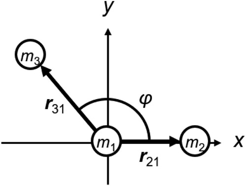
To illustrate this situation, Figure 1 shows a three-atom molecule in which the two bond lengths r₂₁ and r₃₁ are constrained while the angle φ is allowed to change, where r_ij = |r_ij| and r_ij = r_i – r_j. The molecule consists of two rigid subunits: one is the bond between atom 2 and 1 and the other is the bond between atoms 3 and 1. The two units share atom 1 and their motions are not independent; for example, if the motion of one unit is completely frozen, the translational motion of the other unit is also frozen. Let the molecular motion of this molecule be described by the translation of r₁ and the rotations of the two rigid subunits around r₁. Then, the kinetic energy of each atom can be expressed as follows: (16) $\begin{array}{rl}& K_1={\displaystyle \frac{1}{2}{m}_1{\mathit{v}}_1^2,}\\ & K_2={\displaystyle \frac{1}{2}{m}_2({\mathit{v}}_1+{\mathit{\omega }}_2\times {\mathit{r}}_{21}{)}^2,}\\ & K_3={\displaystyle \frac{1}{2}{m}_3({\mathit{v}}_1+{\mathit{\omega }}_3\times {\mathit{r}}_{31}{)}^2,}\end{array}$(16) where ω_i is the angular velocity of atom i around atom 1 and satisfies ${\mathit{v}}_i-{\mathit{v}}_1={\mathit{\omega }}_i\times {\mathit{r}}_{i1}$ under the condition dr_i1/dt = 0. The average kinetic energy of atom i is evaluated by (17) $\begin{array}{rl}{〈K_i〉}_T& ={\int }_{}^{}{K}_i{e}^{-K({\mathit{v}}_1,{\mathit{\omega }}_2,{\mathit{\omega }}_3)/k_{\mathrm{B}}T}d{\mathit{v}}_{1}d{\mathit{\omega }}_{2}d{\mathit{\omega }}_3/\\ & {\int }_{}^{}{e}^{-K({\mathit{v}}_1,{\mathit{\omega }}_2,{\mathit{\omega }}_3)/k_{\mathrm{B}}T}d{\mathit{v}}_{1}d{\mathit{\omega }}_{2}d{\mathit{\omega }}_3,\end{array}$(17) where K = Σ_{i = 1,2,3} K_i is the total kinetic energy of the molecule. After a lengthy calculation, one can finally find the DOFs for atoms 1–3 as (18) $\begin{array}{rl}& g_1\left(\phi \right)=2+{\displaystyle \frac{m_1^2-m_2{m}_3{\sin }^2\phi }{m_{1}M+m_2{m}_3{\sin }^2\phi },}\\ & g_2\left(\phi \right)=2+{\displaystyle \frac{m_1{m}_2+m_2{m}_3{\sin }^2\phi }{m_{1}M+m_2{m}_3{\sin }^2\phi },}\\ & g_3\left(\phi \right)=2+{\displaystyle \frac{m_1{m}_3+m_2{m}_3{\sin }^2\phi }{m_{1}M+m_2{m}_3{\sin }^2\phi },}\end{array}$(18) where M = m₁ + m₂ + m₃. The detail derivation of Equation (18) is described in the Appendix. While the total DOF of the molecule, g₁ + g₂ + g₃ = 7, is constant, the atom DOFs change with time since the angle φ is time dependent. If necessary, g_i can be further averaged over φ as $〈g_i〉=\int g_i\left(\phi \right)f\left(\phi \right)\sin \phi d\phi /\int f\left(\phi \right)\sin \phi d\phi$, where f(φ) = exp[−U(φ)/(k_BT)] is the Boltzmann factor with respect to φ and U(φ) is the potential energy. As one can expect from this simple example, it is rather complicated or even impossible to derive the analytical form of g_i for linked rigid molecules. In such a case, it may be reasonable to calculate 〈K_i〉_T in Equation (4) numerically by carrying out MD simulations of appropriate reference systems.

Figure 1. (Colour online) Three-atom molecule where the lengths of r₂₁ and r₃₁ are constrained, but the angle φ is not.

3. Validation by MD simulation

3.1 Systems and procedures

The expressions of atom DOF derived in Section 2 were examined by conducting MD simulations using the large-scale atomic/molecular massively parallel simulator (LAMMPS) [20]. The expressions for fully rigid molecules, Equations (13)–(15), were validated for a silica–water system as shown in Figure 2, where a bulk liquid composed of 3600 water molecules was sandwiched by two rectangular blocks of silica crystals each consisted of 6 × 6 × 4 unit cells of the α-quartz crystal with the lattice constants a = b = 4.916 Å, c = 5.4054 Å, α = β = 90°, and γ = 120° [21]. The (001) face of silica surface was in contact with the bulk liquid of water, and all Si atoms on the surface were doubly hydroxylated.

Figure 2. (Colour online) Silica–water system, where the rigid SPC/E model is used for water and the O–H bond length of the surface silanol is constrained.

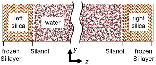
The water molecules were described by the rigid SPC/E model [22], and the DOFs of constituent atoms were calculated with Equation (15). The silica crystals were modelled by the CHARMM-compatible force field of Emami et al. [23] However, the O–H bond length of the surface silanol was additionally constrained to 0.945 Å, and the DOF values of the O and H atoms were calculated with Equation (14). The Rattle algorithm [13] was employed to impose the geometric constraints on water molecules and hydroxyl groups. All non-bonded interactions including those between the water and silica were described by the Lennard-Jones (LJ) and Coulomb interactions. The cut off distance of LJ interaction was set to 12 Å, and the LJ parameters between water and silica atoms were obtained from the Lorentz–Berthelot combining rules. The Coulomb interactions were evaluated using the particle-particle-particle-mesh method [24]. The periodic boundary conditions were imposed in the x and y directions while the boundaries in the z direction were approximately considered non-periodic using the empty volume insertion method [25]. The x and y dimensions, set to L_x = 6a = 29.496 Å and L_y = 6bsinγ = 25.544 Å, respectively, were kept unchanged throughout the MD simulation.

The velocity-Verlet integrator was used with a timestep of 0.1 fs to integrate the equations of motion. The total simulation time was 8 ns, where the temperature of the whole system was controlled at 298.15 K using the Langevin thermostat with a damping coefficient of 0.2 ps. In the first 4 ns, a pressure of 1 atm was applied in the z direction by exerting constant force on the outmost atom layer of the right silica block while freezing the outmost atom layer of the left silica block. In the latter 4 ns, the outmost layer of the right silica block was also frozen, and the temperature profile along the z direction was computed in the last 2 ns.

In an additional simulation, the atom DOF expressions in Equation (18) for the three-atom linked rigid molecule were applied to a semi-flexible water where the two O–H bonds are constrained but the HOH angle varies with time. The water molecule was described by the flexible simple point-charge water model (SPC/Fw) [26], and the O–H bond length was additionally constrained to 0.94 Å. A bulk system with a mass density of 1 g/cm³ was constructed by placing 500 water molecules in a cubic MD box with 24.638 Å on a side, and the three-dimensional periodic boundary conditions were imposed. The MD simulation was conducted for 7 ns employing the velocity-Verlet integrator with a time step of 1 fs, where the system temperature was controlled at 298.15 K using the Langevin thermostat with a damping coefficient of 0.1 ps. The first 2 ns was used for equilibration, and the atom DOFs were calculated from the last 5 ns.

For both the silica–water system and semi-flexible water system, the statistical uncertainty of a physical quantity was estimated by the standard error of mean calculated by dividing the production simulation into five time blocks.

3.2. Results and discussion

From the MD simulation of the silica–water system, the local temperature based on Equation (1) was calculated along the z direction with an interval of Δz= 0.2 Å. The resultant temperature profile near the silica–water interface on the left side is shown in Figure 3. With the new expressions of g_i, Equations (13)–(15), the DOFs of constrained atoms are evaluated as g_H = 2.059 and g_O = 2.941 for silanol, and g_H = 1.5947 and g_O = 2.8106 for water. The Si and O atoms inside the silica crystal are unconstrained, i.e. g_Si = g_O = 3. The temperature profile based on these atom DOF values are plotted in Figure 3(a) by atom type. As expected, the local temperature in every slab is found to be equal to the setting temperature, T_set = 298.15 K. We note that near the boundaries of different regions, the number of atoms in a local volume can be so small that the calculated temperature values deviate significantly from T_set with large statistical errors. Since such data are not reliable, temperature data with the standard error of mean (SEM) greater than 3 K (1% of T_set) are excluded from Figure 3 (However, there are still some regions in Figure 3(a), e.g. at z ∼ 24 Å, where the profile appears to deviate from T_set, albeit only slightly). Since the SEM of 3 K is smaller than the markers, the error bars are not explicitly shown in the figure.

Figure 3. (Colour online) Temperature profile near the silica–water interface on the left side. (a) Profile for each atom type by the new expressions of atom DOF. (b) Profile for each atom type by the conventional approximation. (c) Average of all atom types based on the conventional approximation, where the inset shows the number density of H (dotted curve) and O (solid curve) atoms either in silanol (blue) or water (red). In these figures, the setting temperature is denoted by the grey horizontal line. (d) Profiles of translational and rotational temperatures of surface OH groups and water molecules.

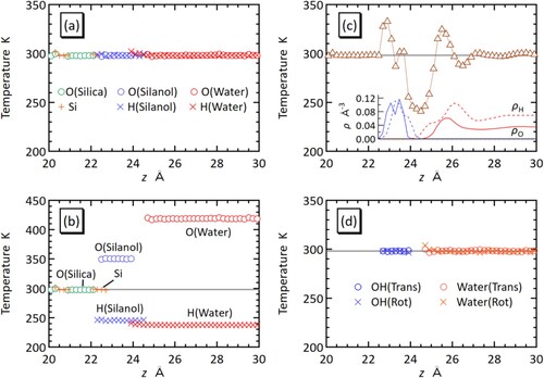
In contrast to the new DOF expressions, if the conventional even-distribution approximation Equation (3) is used, the atom DOFs of the constrained atoms are calculated as g_H = g_O = 2.5 for silanol and g_H = g_O = 2.0 for water. The temperature profile based on these DOF values are shown in Figure 3(b), where the temperature values of the constrained O and H atoms significantly deviate from T_set. The temperature profile in Figure 3(c) is also based on the even-distribution approximation, but it shows the average of all atom types. For z > ∼28 Å, the temperature is close to T_set. In this region, the number density distribution in the inset of Figure 3(c) indicates ρ_H/ρ_O ∼ 2, i.e. the number ratio of H and O atoms in a local slab is close to that in a water molecule, as assumed in the equal-distribution approximation. In this case, the errors in the atom temperature between O and H atoms are cancelled out when their average is taken. For the same reason, in the case of the silanol region, the average atom temperature becomes close to T_set when ρ_H/ρ_O ∼ 1, as is seen at z ∼ 23.5 Å. For other regions, the balance in the number of atoms is broken owing to the inhomogeneous molecular configurations, and as a result, the temperature profile deviates from T_set. Thus, the oscillation in the temperature profile in Figure 3(c) is an artifact of an inappropriate definition of atom DOF, clearly indicating that the even-distribution approximation is not suitable for inhomogeneous systems.

Finally, Figure 3(d) displays the profiles of translational and rotational temperatures calculated by considering surface silanol groups and water as rigid bodies. The profiles are flat with the values near the setting temperature of 298.15 K, confirming that the system is in an equilibrium state.

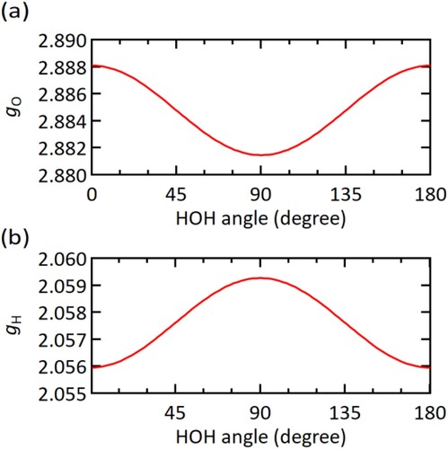
Next, we discuss the result for the semi-flexible water system. The atom DOF expression Equation (18) depends on the instantaneous value of HOH angle φ. However, in the case of water, the large difference in atomic mass between H and O atoms makes the angle dependence ignorable. In Figure 4, the values of g_O and g_H based on Equation (18) are plotted as a function of HOH angle. For both g_O and g_H, the difference between the minimum and maximum is only ∼0.2%. From the MD simulation, the atom DOF values calculated by the time average of the analytic expressions in Equation (18) were g_O = 2.8823 and g_H = 2.0588 with statistical errors of the order of 10⁻⁷. We also calculated the atom DOFs from Equation (4) together with the numerical average of 〈K_i〉_T as g_O = 2.8829 ± 0.0006 and g_H = 2.0587 ± 0.0003. The two results are in good agreement with each other. One may be interested in the extent to which the DOF values depend on statistical ensemble. After the canonical simulation with Langevin thermostat, we conducted a 7.0 ns microcanonical simulation. The average values of atom DOFs in Equation (18) were calculated from the last 5 ns of this simulation as g_O = 2.8823 and g_H = 2.0589 with statistical errors of the order of 10⁻⁷, where the average temperature was 299.09 ± 0.05 K. Thus, the DOF values are insensitive to the difference in statistical ensemble. As we saw throughout the present study, the DOFs of constrained atoms are non-integer in general. This is because geometric constraints make the coordinates of a single atom no longer independent variables of motion. In addition, the value of atom DOF tends to be larger when the atom has higher atomic mass and higher partial inertia moment. For example, suppose a diatomic rigid molecule moving with a translational velocity V without rotation. Because of the rigid-body constraint, the velocities of two constituent atoms 1 and 2 must also be V. If the kinetic energy of atom i, m_iV²/2, is equated to g_ik_BT/2 assuming that these atoms have the same instantaneous temperature T, the atom DOF g_i must be proportional to m_i. This simple example, if not rigorous, would be helpful to intuitively understand why non-integer and non-uniform DOFs are assigned to constrained atoms.

Figure 4. (Colour online) Atom DOFs defined by Equation (18) for (a) O and (b) H atoms in the semi-flexible water as a function of HOH angle.

4. Conclusion

In the present study, we derived expressions for the DOF of constrained atoms, which is necessary for the calculation of local temperature in MD simulation systems of fully or partially rigid molecules. The expressions are based on statistical mechanics to ensure that in an equilibrium state, all constrained atoms have the same temperature as the whole system. The conventionally used approximation of reducing the atom DOF by 1/2 per one distance constraint can be used if a simulation system is spatially homogeneous. However, recent MD simulations often have to deal with systems that do not satisfy this condition, such as nanostructures and interfaces of different phases, and in such cases, the use of the new atom DOF expressions is essential.

Disclosure statement

No potential conflict of interest was reported by the author(s).

Correction Statement

This article has been corrected with minor changes. These changes do not impact the academic content of the article.

Additional information

Funding

This work was supported by JST CREST [grant number JPMJCR17I2], Japan. Numerical simulations were performed on the Supercomputer system 'AFI-NITY' at the Advanced Fluid Information Research Center, Institute of Fluid Science, Tohoku University.

Appendix

In this appendix, we derive Equation (18), the atom DOF for the three-atom molecule as shown in Figure 1, in which atom 1 has two constrained bonds with atom 2 and 3. The kinetic energy of atom i is given by Equation (16) in terms of the relative position vector r_i1 = r_i − r₁ and the angular velocity ω_i around atom 1. Applying the relation $({\mathit{\omega }}_i\times {\mathit{r}}_{i1}{)}^{\mathrm{T}}({\mathit{\omega }}_j\times {\mathit{r}}_{j1})={\mathit{\omega }}_i^{\mathrm{T}}({\mathit{r}}_{i1}^T{\mathit{r}}_{j1}-{\mathit{r}}_{i1}{\mathit{r}}_{j1}^T){\mathit{\omega }}_j$ to the atom kinetic energy, the total kinetic energy of the molecule can be transformed into the following form: (19) $\begin{array}{rl}K({\mathit{v}}_1,{\mathit{\omega }}_2,{\mathit{\omega }}_3)& ={\displaystyle \frac{1}{2}{m}_1{\mathit{v}}_1^2+{\displaystyle \frac{1}{2}{m}_2({\mathit{v}}_1+{\mathit{\omega }}_2\times {\mathit{r}}_{21}{)}^2+{\displaystyle \frac{1}{2}{m}_3({\mathit{v}}_1+{\mathit{\omega }}_3\times {\mathit{r}}_{31}{)}^2}}}\\ & ={\displaystyle \frac{1}{2}M{\mathit{V}}^2+{\displaystyle \frac{1}{2}{\mathit{\omega }}_2^{\mathrm{T}}{\mathbf{I}}_2{\mathit{\omega }}_2+{\displaystyle \frac{1}{2}{\mathit{\omega }}_3^{\mathrm{T}}{\mathbf{I}}_3{\mathit{\omega }}_3-{\mathit{\omega }}_2^{\mathrm{T}}{\mathbf{I}}_{32}{\mathit{\omega }}_3,}}}\end{array}$(19) where M = m₁+ m₂+ m₃ is the total mass of the molecule and (20) $\mathit{V}={\mathit{v}}_1+(m_2{\mathit{\omega }}_2\times {\mathit{r}}_{21}+m_3{\mathit{\omega }}_3\times {\mathit{r}}_{31})/M$(20) is the centre of mass of the molecule expressed in terms of v₁, ω₂, and ω₃. Here, the partial inertia tensors are defined in a slightly different way from Equation (7) as (21) $\begin{array}{rl}{\mathbf{I}}_i& =({\mathit{r}}_{i1}^T{\mathit{r}}_{i1}-{\mathit{r}}_{i1}{\mathit{r}}_{i1}^T)m_i(M-m_i)/M,\\ {\mathbf{I}}_{ij}& =({\mathit{r}}_{i1}^T{\mathit{r}}_{j1}-{\mathit{r}}_{i1}{\mathit{r}}_{j1}^T)m_i{m}_j/M.\end{array}$(21) We note that the centre of rotation in these tensors is r₁ rather than the molecular centre of mass, and that I_i is a symmetric matrix but I_ij is not. By completing the square, Equation (19) can be further transformed as (22) $K(\mathit{V},{{\mathit{\omega }}^{\mathrm{\prime }}}_2,{{\mathit{\omega }}^{\mathrm{\prime }}}_3)=M{\mathit{V}}^2/2+{{\mathit{\omega }}^{\mathrm{\prime }}}_2^2/2+{{\mathit{\omega }}^{\mathrm{\prime }}}_3^2/2$(22) where (23) $\begin{array}{rl}{{\mathit{\omega }}^{\mathrm{\prime }}}_2& =({\mathbf{I}}_2^{1/2}{\mathit{\omega }}_2-{\mathbf{I}}_2^{-1/2}{\mathbf{I}}_{32}{\mathit{\omega }}_3),\\ {{\mathit{\omega }}^{\mathrm{\prime }}}_3& ={\mathbf{B}}^{1/2}{\mathit{\omega }}_3,\\ \mathbf{B}& ={\mathbf{I}}_3-{\mathbf{I}}_{32}^{\mathrm{T}}{\mathbf{I}}_2^{-1}{\mathbf{I}}_{32}={\mathbf{B}}^{\mathrm{T}}.\end{array}$(23) Correspondingly, the integral variables v₁, ω₂, and ω₃ of the average kinetic energy of atom i in Equation (17) are changed to V, ω′₂, and ω′₃ as (24) ${〈K_i〉}_T={\int }_{}^{}{K}_i{e}^{-K(\mathit{V},{{\mathit{\omega }}^{\mathrm{\prime }}}_2,{{\mathit{\omega }}^{\mathrm{\prime }}}_3)/k_{\mathrm{B}}T}d\mathit{V}d{{\mathit{\omega }}^{\mathrm{\prime }}}_{2}d{{\mathit{\omega }}^{\mathrm{\prime }}}_3/{\int }_{}^{}{e}^{-K(\mathit{V},{{\mathit{\omega }}^{\mathrm{\prime }}}_2,{{\mathit{\omega }}^{\mathrm{\prime }}}_3)/k_{\mathrm{B}}T}d\mathit{V}d{{\mathit{\omega }}^{\mathrm{\prime }}}_{2}d{{\mathit{\omega }}^{\mathrm{\prime }}}_3$(24)

The Jacobian of this transformation cancels between the numerator and denominator and is not shown explicitly. As for atom 1, using Equations (20) and (23), the atom kinetic energy K₁ = m₁v₁²/2 is rewritten as a function of V, ω′₂, and ω′₃ as: (25) $\begin{array}{rl}{K}_1& ={\displaystyle \frac{1}{2}{m}_1(\mathit{V}-(m_2{\mathit{\omega }}_2\times {\mathit{r}}_{21}+m_3{\mathit{\omega }}_3\times {\mathit{r}}_{31})/M{)}^2}\\ & ={\displaystyle \frac{1}{2}{m}_1{\mathit{V}}^2+{\displaystyle \frac{1}{2}{\displaystyle \frac{m_1{m}_2}{M(M-m_2)}{{\mathit{\omega }}^{\mathrm{\prime }}}_2^2}}}\\ & +{\displaystyle \frac{1}{2}{{\mathit{\omega }}^{\mathrm{\prime }}}_3^{\mathrm{T}}{\mathbf{B}}^{-1/2}{\mathbf{C}}_1{\mathbf{B}}^{-1/2}{{\mathit{\omega }}^{\mathrm{\prime }}}_3+F_1(\mathit{V},{{\mathit{\omega }}^{\mathrm{\prime }}}_2,{{\mathit{\omega }}^{\mathrm{\prime }}}_3)}\end{array}$(25) where (26) ${\mathbf{C}}_1=\left[{\displaystyle \frac{m_1(2M-m_2)}{M(M-m_2)}{\mathbf{I}}_{32}^{\mathrm{T}}{\mathbf{I}}_2^{-1}{\mathbf{I}}_{32}-{\displaystyle \frac{m_1{m}_3}{M(M-m_3)}{\mathbf{I}}_3}}\right]$(26)

In the right-hand side of Equation (25), F₁ represents the collection of terms that depend linearly on V, ω′₂, and ω′₃ and therefore becomes zero after integrating with these variables in Equation (24). Inserting K₁ in Equation (25) into Equation (24) gives the equilibrium average of the kinetic energy as (27) ${〈K_1〉}_T={\displaystyle \frac{k_{\mathrm{B}}T}{2}\left[{\displaystyle \frac{3m_1}{M}+{\displaystyle \frac{2m_1{m}_2}{M(M-m_2)}+\mathrm{T}\mathrm{r}[{\mathbf{C}}_1{\mathbf{B}}^{-1}]}}\right]}$(27) where the Tr[A] means the trance of a matrix A. The third term in the right-hand side of Equation (27) can be obtained as follows: (28) $\begin{array}{rl}{〈K_i〉}_T^{\left(3\right)}& ={\displaystyle \frac{1}{2}{\int }_{}^{}{{\mathit{\omega }}^{\mathrm{\prime }}}_3^{\mathrm{T}}{\mathbf{B}}^{-1/2}{\mathbf{C}}_1{\mathbf{B}}^{-1/2}{{\mathit{\omega }}^{\mathrm{\prime }}}_3{e}^{-{{\mathit{\omega }}^{\mathrm{\prime }}}_3^2/2k_{\mathrm{B}}T}d{{\mathit{\omega }}^{\mathrm{\prime }}}_3}/{\int }_{}^{}{e}^{-{{\mathit{\omega }}^{\mathrm{\prime }}}_3^2/2k_{\mathrm{B}}T}d{{\mathit{\omega }}^{\mathrm{\prime }}}_3\\ & ={\displaystyle \frac{1}{2}{\int }_{}^{}{{\mathit{\omega }}^{\mathrm{\prime }\mathrm{\prime }}}_3^{\mathrm{T}}{\mathbf{P}}^{\mathrm{T}}{\mathbf{B}}^{-1/2}{\mathbf{C}}_1{\mathbf{B}}^{-1/2}\mathbf{P}{{\mathit{\omega }}^{\mathrm{\prime }\mathrm{\prime }}}_3{e}^{-{{\mathit{\omega }}^{\mathrm{\prime }\mathrm{\prime }}}_3^2/2k_{\mathrm{B}}T}d{{\mathit{\omega }}^{\mathrm{\prime }\mathrm{\prime }}}_3}/{\int }_{}^{}{e}^{-{{\mathit{\omega }}^{\mathrm{\prime }\mathrm{\prime }}}_3^2/2k_{\mathrm{B}}T}d{\mathit{\omega }}^{\mathrm{\prime }\mathrm{\prime }}\\ & ={\displaystyle \frac{k_{\mathrm{B}}T}{2}\mathrm{T}\mathrm{r}[{\mathbf{P}}^{\mathrm{T}}{\mathbf{B}}^{-1/2}{\mathbf{C}}_1{\mathbf{B}}^{-1/2}\mathbf{P}],}\end{array}$(28) where we changed the integral variables as ω′₃ = Pω″₃ with an orthogonal matrix P, i.e. P^TP = 1, so that P^TB^−1/2C₁B^−1/2P is a 2 × 2 diagonal matrix. Then, one can perform the integrations with respect to the two components of ω″₃ separately to show the last equality in Equation (28). The result in Equation (27) is finally obtained using the property that two matrices X and Y are interchangeable in a trace as Tr[XY] = Tr[YX].

The average kinetic energy of atom 2 can be derived analogously. The atom kinetic energy K₂ = m₂v₂²/2 in terms of V, ω′₂, and ω′₃ is written as (29) $K_2={\displaystyle \frac{1}{2}{m}_2{\mathit{V}}^2+{\displaystyle \frac{M-m_2}{2M}{{\mathit{\omega }}^{\mathrm{\prime }}}_2^2+{\displaystyle \frac{1}{2}{{\mathit{\omega }}^{\mathrm{\prime }}}_3^{\mathrm{T}}{\mathbf{B}}^{-1/2}{\mathbf{C}}_2{\mathbf{B}}^{-1/2}{{\mathit{\omega }}^{\mathrm{\prime }}}_3+F_2(\mathit{V},{{\mathit{\omega }}^{\mathrm{\prime }}}_2,{{\mathit{\omega }}^{\mathrm{\prime }}}_3),}}}$(29) where F₂ is linear in V, ω′₂, and ω′₃ and does not contribute to 〈K₂〉_T, and (30) ${\mathbf{C}}_2={\displaystyle \frac{(M-m_2)}{2M}\left[{\displaystyle \frac{m_2{m}_3}{(M-m_2)(M-m_3)}{\mathbf{I}}_3-{\mathbf{I}}_{32}^{\mathrm{T}}{\mathbf{I}}_2^{-1}{\mathbf{I}}_{32}}\right]}$(30)

The equilibrium average of K₂ is calculated as (31) ${〈K_2〉}_T={\displaystyle \frac{k_{\mathrm{B}}T}{2}\left[{\displaystyle \frac{3m_2}{M}+{\displaystyle \frac{(M-m_2)}{2M}+\mathrm{T}\mathrm{r}[{\mathbf{C}}_2{\mathbf{B}}^{-1}]}}\right]}$(31)

Since atom 2 and 3 are mathematically equivalent in Equation (19), the expression of 〈K₃〉_T can be obtained just by exchanging the indices 2 and 3 in Equation (31) and the variables therein.

The matrices C₁, C₂ and B are calculated from I_i and I_ij. The rank-2 matrices I_i and I_ij can be first constructed as 3 × 3 matrices using Equation (21) in an any convenient coordinate system, e.g. that in Figure 1. Then, we find an orthogonal matrix P_i such that${{\mathbf{I}}^{\mathrm{\prime }\mathrm{\prime }}}_i={\mathbf{P}}_i^{\mathrm{T}}{\mathbf{I}}_i{\mathbf{P}}_i$ becomes a 3 × 3 diagonal matrix (A double prime is used to denote a matrix or a vector in the coordinate system where I_i is diagonalised). The 2 × 2 form of ${{\mathbf{I}}^{\mathrm{\prime }\mathrm{\prime }}}_i$ can be obtained just by removing a row and a column whose components are all zeros. Since the conversion by P_i corresponds to the coordinate transform ${\mathit{\omega }}_i={\mathbf{P}}_i{{\mathit{\omega }}^{\mathrm{\prime }\mathrm{\prime }}}_i$ in Equation (19), I₃₂ is converted into ${{\mathbf{I}}^{\mathrm{\prime }\mathrm{\prime }}}_{32}={\mathbf{P}}_2^{\mathrm{T}}{\mathbf{I}}_{32}{\mathbf{P}}_3$, which is also diagonal and can be reduced to a 2 × 2 form. If we choose the coordinate system in Figure 1, we have r₂₁ = (r₂₁, 0, 0)^T and r₃₁ = (r₃₁cosφ, r₃₁sinφ, 0)^T. The orthogonal matrix P₂ is the 3 × 3 unit matrix and P₃ is given by (32) ${\mathbf{P}}_3=\left(\begin{array}{ccc}\cos \phi & -\sin \phi & 0\\ \sin \phi & \cos \phi & 0\\ 0& 0& 1\end{array}\right)$(32)

The partial inertia tensors are obtained as follows: (33) $\begin{array}{rl}& {{\mathbf{I}}^{\mathrm{\prime }\mathrm{\prime }}}_2={\displaystyle \frac{m_2(M-m_2)r_{21}^2}{M}\left(\begin{array}{cc}1& 0\\ 0& 1\end{array}\right),}\\ & {{\mathbf{I}}^{\mathrm{\prime }\mathrm{\prime }}}_3={\displaystyle \frac{m_3(M-m_3)r_{31}^2}{M}\left(\begin{array}{cc}1& 0\\ 0& 1\end{array}\right),}\\ & {{\mathbf{I}}^{\mathrm{\prime }\mathrm{\prime }}}_{32}={\displaystyle \frac{m_2{m}_3{r}_{21}{r}_{31}}{M}\left(\begin{array}{cc}1& 0\\ 0& \cos \phi \end{array}\right).}\end{array}$(33)

These matrices are used to evaluate the average kinetic energy in Equations (27) and (31), which, together with (4), finally leads to Equation (18). The g₃ can be obtained from g₂ by exchanging indices 2 and 3.

Finally, it is worth showing the atom DOF expressions for the case of a four-atom molecule where atom 1 has three constrained bonds with atom 2, 3, and 4, to see how the expressions become more complicated by the addition of one more atom in the molecule. In the same way as that for the three-atom molecule above, the DOFs of atom 1 and 2 in the four-atom molecule are derived as follows: (34) $\begin{array}{rl}{g}_1& ={\displaystyle \frac{3m_1}{M}+{\displaystyle \frac{2m_1{m}_2}{M(M-m_1)}-4{\displaystyle \frac{(2M-m_2)m_1}{M(M-m_2)}+\mathrm{T}\mathrm{r}\left[{\mathbf{X}}_1\right],}}}\\ g_2& ={\displaystyle \frac{3m_2}{M}+{\displaystyle \frac{(M-m_2)}{M}\left(6+\mathrm{T}\mathrm{r}\left[{\mathbf{X}}_2\right]\right),}}\end{array}$(34) where M = m₁ + m₂ + m₃ + m₄ and (35) $\begin{array}{rl}& {\mathbf{X}}_1=\left[{\nu }_4{\mathbf{I}}_4+{\nu }_3{\mathbf{D}\mathbf{B}}_3^{-1}{\mathbf{I}}_3{\mathbf{B}}_3^{-1}{\mathbf{D}}^{\mathrm{T}}-2{\mathbf{I}}_{34}{\mathbf{B}}_3^{-1}{\mathbf{D}}^{\mathrm{T}}{m}_1/(M-m_2)\right]{\mathbf{E}}^{-1}+{\nu }_3{\mathbf{I}}_3{\mathbf{B}}_3^{-1},\\ & {\mathbf{X}}_2=\left[q_{42}{\mathbf{I}}_4+q_{32}{\mathbf{I}}_3{\mathbf{D}\mathbf{B}}_3^{-2}{\mathbf{D}}^{\mathrm{T}}+2{\mathbf{I}}_{34}{\mathbf{B}}_3^{-1}{\mathbf{D}}^{\mathrm{T}}M/(M-m_2)\right]{\mathbf{E}}^{-1}+q_{32}{\mathbf{I}}_3{\mathbf{B}}_3^{-1},\\ & {\mathbf{B}}_i={\mathbf{I}}_i-{\mathbf{I}}_{i2}^{\mathrm{T}}{\mathbf{I}}_2^{-1}{\mathbf{I}}_{i2},\\ & \mathbf{D}={\mathbf{I}}_{34}+{\mathbf{I}}_{42}^{\mathrm{T}}{\mathbf{I}}_2^{-1}{\mathbf{I}}_{32},\\ & \mathbf{E}={\mathbf{B}}_4-{\mathbf{D}\mathbf{B}}_3^{-1}{\mathbf{D}}^{\mathrm{T}},\\ & {\nu }_i={\displaystyle \frac{m_1(2M-m_2-m_i)}{(M-m_2)(M-m_i)},}\\ & q_{ij}={\displaystyle \frac{m_i{m}_j}{(M-m_i)(M-m_j)}-1.}\end{array}$(35)

The meaning of I_i and I_ij are the same as in Equation (21). In the expression of g₂, exchanging indices 2 and 3 yields the expression for g₃, and exchanging indices 2 and 4 yields that for g₄. Although it is possible to rewrite g_i, as in Equation (18), in terms of m_i and the three angles to specify relative orientations of r₂₁, r₃₁, r₄₁, the expression contains too many terms to be wieldy. Therefore, it is better to use Equation (34) when one calculates g_i numerically. The three-atom and four-atom molecules above as well as fully rigid molecules cover all cases of geometric constraints implemented in LAMMPS.

References

- Allen MP, Tildesley DJ. Computer simulation of liquids. 2nd ed. Oxford University Press; 2017. doi:10.1093/oso/9780198803195.001.0001
- Ponce V, Galvez-Aranda DE, Seminario JM. Analysis of an all-solid state nanobattery using molecular dynamics simulations under an external electric field. Phys Chem Chem Phys. 2021;23:597–606. doi:10.1039/D0CP02851G
- Zhao B, Zhao P, Wu J, et al. Investigation on surface generation mechansim of single-crystal silicon in grinding: surface crystal orientation effect. SSRN Electron J. 2022;34:105125. doi:10.2139/ssrn.4267745
- Matsubara H, Kikugawa G, Bessho T, et al. Non-equilibrium molecular dynamics simulation as a method of calculating thermodynamic coefficients. Fluid Phase Equilib. 2016;421:1–8. doi:10.1016/j.fluid.2016.03.019
- Algaer EA, Müller-Plathe F. Molecular dynamics calculations of the thermal conductivity of molecular liquids, polymers, and carbon nanotubes. Soft Mater. 2012;10:42–80. doi:10.1080/1539445X.2011.599699
- Liang Z, Hu M. Tutorial: determination of thermal boundary resistance by molecular dynamics simulations. J Appl Phys. 2018;123:191101. doi:10.1063/1.5027519
- Oda K, Miyagawa H, Kitamura K. How does the electrostatic force cut-off generate non-uniform temperature distributions in proteins? Mol Simul. 1996;16:167–177. doi:10.1080/08927029608024070
- Eastwood MP, Stafford KA, Lippert RA, et al. Equipartition and the calculation of temperature in biomolecular simulations. J Chem Theory Comput. 2010;6:2045–2058. doi:10.1021/ct9002916
- Uranagase M, Ogata S. Nonequilibrium molecular dynamics method based on coarse-graining formalism: application to a nonuniform temperature field system. Phys Rev E. 2021;104:65301. doi:10.1103/PhysRevE.104.065301
- Templeton JA, Jones RE, Wagner GJ. Application of a field-based method to spatially varying thermal transport problems in molecular dynamics. Model Simul Mater Sci Eng. 2010;18:085007. doi:10.1088/0965-0393/18/8/085007.
- Kräutler V, Van Gunsteren WF, Hünenberger PH. A fast SHAKE algorithm to solve distance constraint equations for small molecules in molecular dynamics simulations. J Comput Chem. 2001;22:501–508. https://doi.org/10.1002/1096-987X(20010415)22:5<501::AID-JCC1021>3.0.CO;2-V
- Zhang M, Lussetti E, de Souza LES, et al. Thermal conductivities of molecular liquids by reverse nonequilibrium molecular dynamics. J Phys Chem B. 2005;109:15060–15067. doi:10.1021/jp0512255
- Andersen HC. Rattle: A “velocity” version of the shake algorithm for molecular dynamics calculations. J Comput Phys. 1983;52:24–34. doi:10.1016/0021-9991(83)90014-1
- Kamberaj H, Low RJ, Neal MP. Time reversible and symplectic integrators for molecular dynamics simulations of rigid molecules. J Chem Phys. 2005;122:224114. doi:10.1063/1.1906216.
- Mao Y, Zhang Y. Thermal conductivity, shear viscosity and specific heat of rigid water models. Chem Phys Lett. 2012;542:37–41. doi:10.1016/j.cplett.2012.05.044
- Matsubara H, Kikugawa G, Ohara T. Comparison of molecular heat transfer mechanisms between water and ammonia in the liquid states. Int J Therm Sci. 2021;161:106762. doi:10.1016/j.ijthermalsci.2020.106762
- Prohaska T, Irrgeher J, Benefield J, et al. Standard atomic weights of the elements 2021 (IUPAC technical report). Pure Appl Chem. 2022;94:573–600. doi:10.1515/pac-2019-0603
- Sirk TW, Moore S, Brown EF. Characteristics of thermal conductivity in classical water models. J Chem Phys. 2013;138:064505. doi:10.1063/1.4789961.
- Forester TR, Smith W. SHAKE, rattle, and roll: efficient constraint algorithms for linked rigid bodies. J Comput Chem. 1998;19:102–111. doi:10.1002/(SICI)1096-987X(19980115)19:1<102::AID-JCC9>3.0.CO;2-T
- Thompson AP, Aktulga HM, Berger R, et al. LAMMPS - a flexible simulation tool for particle-based materials modeling at the atomic, meso, and continuum scales. Comput Phys Commun. 2022;271:108171. doi:10.1016/j.cpc.2021.108171
- Levien L, Prewitt CT, Weidner DJ, et al. Structure and elastic properties of quartz at pressure. Am Mineral. 1980;65:920–930.
- Berendsen HJC, Grigera JR, Straatsma TP. The missing term in effective pair potentials. J Phys Chem. 1987;91:6269–6271. doi:10.1021/j100308a038
- Emami FS, Puddu V, Berry RJ, et al. Erratum: force field and a surface model database for silica to simulate interfacial properties in atomic resolution. Chem Mater. 2016;28:406–407. doi:10.1021/acs.chemmater.5b04760
- Deserno M, Holm C. How to mesh up Ewald sums. II. An accurate error estimate for the particle-particle-particle-mesh algorithm. J Chem Phys. 1998;109:7694–7701. doi:10.1063/1.477415
- Yeh IC, Berkowitz ML. Ewald summation for systems with slab geometry. J Chem Phys. 1999;111:3155–3162. doi:10.1063/1.479595
- Wu Y, Tepper HL, Voth GA. Flexible simple point-charge water model with improved liquid-state properties. J Chem Phys. 2006;124:024503. doi:10.1063/1.2136877.