Determining Reliability of Daily Measures: An Illustration with Data on Teacher Stress

ABSTRACT

Intensive longitudinal data is increasingly used to study state-like processes such as changes in daily stress. Measures aimed at collecting such data require the same level of scrutiny regarding scale reliability as traditional questionnaires. The most prevalent methods used to assess reliability of intensive longitudinal measures are based on the generalizability theory or a multilevel factor analytic approach. However, the application of recent improvements made for the factor analytic approach may not be readily applicable for all researchers. Therefore, this article illustrates a five-step approach for determining reliability of daily data, which is one type of intensive longitudinal data. First, we show how the proposed reliability equations are applied. Next, we illustrate how these equations are used as part of our five-step approach with empirical data, originating from a study investigating changes in daily stress of secondary school teachers. The results are a within-level (ω^w), between-level (ω^b) reliability score. Mplus syntax for these examples is included and discussed. As such, this paper anticipates on the need for comprehensive guides for the analysis of daily data.

1. Introduction

Due to technological advances, intensive longitudinal data collection methods have flourished. These data can now be collected in a less intrusive manner, causing fewer hinderances for participants (Cranford et al., 2006; McNeish & Hamaker, 2019; Mehl, Conner, & Csikszentmihalyi, 2012). Traditional longitudinal data are characterized by a limited number of repeated measures with large time intervals in between. New data collection techniques (e.g., using phone or tablet applications) have resulted in data with more measurement ocassions, which are spaced in much closer proximity to each other (McNeish & Hamaker, 2019). These so-called intensive longitudinal data enable the investigation of dynamics of state-like processes, such as the daily changes in teachers’ stress. However, establishing scale reliability of time-intensive measures (e.g., daily measures) is a potential challenge for many researchers since multiple approaches exist.

Data collected with daily measures have a nested structure, because multiple measurement occasions are nested within the same person. Currently, two different techniques are commonly used to analyze scale reliability with nested data. The first of these techniques is the generalizability theory approach (Brennan, 2001). This approach decomposes the total variance of scales into elements of time, item, and person. These different sources of variance are then used to assess, for example, within-level (within-person) reliability of change over time (Bolger & Laurenceau, 2013; Mehl et al., 2012). Although the use of the generalizability theory allows for the assessment of reliability for between and within-level change, it relies on assumptions that might not be fully supported by the data. For example, this approach assumes that all items have the same degree of association with the true score (Bolger & Laurenceau, 2013) and that the error variance is the same across items (Shrout & Lane, 2012).

The second technique often employed is a factor analytic approach. This approach has benefits over the use of the generalizability approach, because it is more flexible with respect to how associations of items with the true score and error variances are modeled. Similar to the generalizability theory approach, a multilevel confirmatory factor analysis (MCFA) can also be used to obtain elements of variance in order to determine level-specific reliability of a set of items for time (within-level) and person (between-level) (Geldhof, Preacher, & Zyphur, 2014).

In the MCFA literature, it is increasingly acknowledged that the appropriate specification of the MCFA depends on the level of interest (within- or between-persons) (Stapleton et al., 2016). Within the context of daily measures, the answers given each day will always depend on the person providing them. Therefore, the interest will be in both differences within-persons over time and differences between-persons. This means that modeling daily data ideally requires fitting a two-level model with equal factor structure at the two levels, and equality constraints across levels on the factor loadings (Jak, 2019). This type of model, where the within- and between factors reflect the within- and between components of the same latent variable is labeled a configural model by Stapleton et al. (2016).

Recently, Lai (2021) contributed to the estimation of reliability with the MCFA approach in two ways. First, Lai provided improved reliability equations specifically for different types of multilevel models, including models that focus on the importance of both the within- and between-level. Second, in MCFA, reliability at the between-level is often assessed for the latent indicator scores (c.f., Geldhof et al., 2014), which can result in serious overestimation of the reliability. This is due to the fact that latent scores ignore the measurement error present in observed scores (Lai, 2021). Lai has addressed this issue of overestimation at the between-level by presenting adjusted equations that lead to reliability estimates for the observed scores at each level. In the next section we will consider both these refinements in greater detail.

Due to the technical nature of such papers, these recently improved MCFA techniques may not be easily applicable by researchers and practitioners who aim to determine the reliability of daily data. Therefore, in this article we provide a comprehensive 5-step illustration for the assessment of reliability with daily intensive longitudinal data. To this end we use example calculations and empirical data which were collected with a daily work-related stress measure for secondary school teachers. Lastly, given that the generalizability theory method is also a commonly used approach for these kinds of data, we will compare the resulting reliability indices from the MCFA method with those derived from the generalizability theory approach.

2. Theoretical Framework

The following section provides an overview of how reliability for single and multilevel factor models is defined. We continue by providing example calculations for determining reliability indices with a multilevel model. Lastly, we introduce five steps that, in combination with additional examples based on empirical data, will aid researchers and practitioners in determining scale reliability indices (ω^b and ω^w) for intensive longitudinal measures.

2.1. Reliability in Single-Level Factor Models

Using confirmatory factor analysis (CFA) has become the standard for determining the dimensionality and reliability of scores in the field of psychology (Brown, 2015). Assessing reliability with a CFA in single-level data can be done with several different indices. Unlike the commonly used internal consistency coefficient α (Cronbach, 1951), ω (McDonald, 1999) does not assume that all factor loadings of items contribute equally to the latent construct.

Values for ω range from zero to one, where values closer to one are indicative of better scale reliability. The actual value of ω can be interpreted as the proportion of (summed or averaged) variance in the scale scores accounted for by the latent variable that is common to all the indicators (Cronbach, 1951; McDonald, 1999). Although sought after, currently, no justifiable thresholds exist that can be used to judge whether a scale has poor, good or excellent reliability (see Peters (2014) for a discussion on this topic).

Figure 1 shows an example of a single-level factor model with illustrative values for each parameter. Using a single-level factor analytic approach, assuming no covariances between residual factors,¹ composite reliability ω, for a single construct that is measured with p items, is then defined as:

(1) $\omega =\frac{{\left({\sum }_i^p{\lambda }_i\right)}^2\mathrm{\Phi }}{{\left({\sum }_i^p{\lambda }_i\right)}^2\mathrm{\Phi }+{\sum }_i^p{\theta }_i}$(1)

Figure 1. A single-level CFA with example factor loadings and residual variances for each indicator.

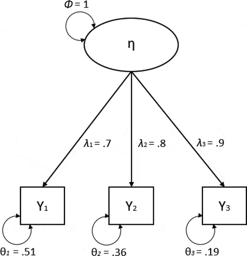
Where i indexes the item, λ represents a factor loading, Φ represents factor variance, and θ represents residual item variance. As the equation shows, composite reliability is determined as the ratio of the common indicator variance over the total indicator variance.

Suppose that the factor variance is fixed to 1 for model identification (Kline, 2011). Using these values, we can determine the reliability of this scale by inserting them in Equation (1)(1) $\omega =\frac{{\left({\sum }_i^p{\lambda }_i\right)}^2\mathrm{\Phi }}{{\left({\sum }_i^p{\lambda }_i\right)}^2\mathrm{\Phi }+{\sum }_i^p{\theta }_i}$(1) , resulting in a reliability of .84:

$\omega =\frac{{\left(0.70+0.80+0.90\right)}^{2}1}{{\left(0.70+0.80+0.90\right)}^{2}1+\left(0.51+0.36+0.19\right)}=.84.$

This means that 84% of the total variance in the scale scores is accounted for by the common factor.

2.2. Reliability in Multilevel Factor Models

In educational and psychological research, data often have a nested structure, where lower level units are said to be nested in higher level units. For instance, students may be nested in classrooms, or patients may be nested in hospitals. With daily measures of individuals on several days, measurement occasions are nested in individuals. Likewise, the empirical data used in the example presented here, are collected from the same individual teachers during 15 measurement occasions. These occasions are nested within each teacher and are therefore at the within (lower) level, while the teachers are at the between (higher) level. MCFA allows for different models for variances and covariances of within-person differences and between-person differences (Muthén, 1994). In this article we focus on two-level structures of occasions (Level 1, or the within-level) in individuals (Level 2, or the between-level).

Figure 2 provides a graphical display of a two-level factor model in the so-called within/between formulation (Schmidt, 1969). In such a two-level CFA, the item scores are decomposed into (latent) within-level and between-level components, represented by the dashed circles connected to the observed variables (see Lüdtke et al., 2008). The between-level part models the covariance structure at the individual level, thereby explaining differences between individuals. The interpretation of this part of the model is comparable to a single-level CFA. The within-level part models the covariance structure at the measurement occasion-level, explaining differences within individuals between time points. In this example, the occasion-level is representative of state-like characteristics because it shows the daily changes of individuals their conditions. The individual-level is then referring to the trait-like characteristics of individuals, because they are an aggregate of the daily measures, and represent a more stable (i.e., long-term), personality-like measure.

Figure 2. A multilevel configural model with example factor loadings, residual variances, and factor variance.

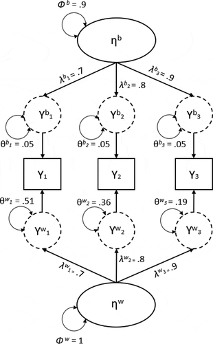
Geldhof et al. (2014) extended the existing method of determining ω to two-level models, resulting in within-level (ω^w) and between-level (ω^b) reliability indices. This approach has been used by, for example, Sadikaj, Wright, Dunkley, Zuroff, and Moskowitz (2019) to estimate reliability with intensive longitudinal data. However, Lai (2021) recently pointed out that the reliability indices proposed by Geldhof et al. (2014), actually do not reflect the reliability of observed test scores. That is, the ω^b proposed by Geldhof et al. reflects the reliability of the latent-error free item means of the clusters (the dashed circles at the between-level in Figure 2). In practice, the observed sample mean of the item in a cluster will be different from the latent-error free cluster mean, due to sampling error. In order to estimate the reliability of the observed cluster means, the sampling error variance of the observed cluster means must be taken into account. The formulas provided by Lai (2021) add this variance component to the total variance when estimating the reliability at the between-level, thereby avoiding overestimation of scale reliability.

2.3. Calculating Scale Reliability with Daily Data

Suppose that researchers are investigating teacher stress using daily intensive longitudinal data. They would probably like to interpret the between-level common factor as the stable part of the stress-factor, and the within-level common factor as the time-varying part of the stress-factor. Here, the within-level variance then reflects the changing state of the individual (Sadikaj et al., 2019). When one is interested in the within-level and between-level components of the same common factor “stress,” the ideal multilevel factor model is a so-called configural model (Stapleton et al., 2016). In a configural multilevel factor model, the within- and between-level factors reflect the within- and between components of the same latent variable. Therefore, the same factor structure applies at both these levels and the factor loadings are equal across levels (Asparouhov & Muthen, 2012; Mehta & Neale, 2005; Rabe-Hesketh, Skrondal, & Pickels, 2004). Since measurement occasions cannot exist without the person-level, we argue that this two-factor model with cross-level equality constraints is the most appropriate model for intensive longitudinal data. Lai (2021) provided equations to determine within-level (ω^w) and between-level (ω^b) reliability estimates specifically for configural models. We will present example calculations for each of these reliability indices in the remainder of this section.

The following equation for determining within-level reliability in a configural model is used:

(2) ${\omega }^w=\frac{{\left({\sum }_i^p{\lambda }_i\right)}^2{\mathrm{\Phi }}^w}{{\left({\sum }_i^p{\lambda }_i\right)}^2{\mathrm{\Phi }}^w+{\sum }_{i=1}^p{{\theta }^w}_i}$(2)

where superscript w refers to the within-level. Note that the factor loadings (λ) do not have a level-specific superscript because the factor loadings are constrained to be equal across levels.

Comparing this within-level omega Equation (2)(2) ${\omega }^w=\frac{{\left({\sum }_i^p{\lambda }_i\right)}^2{\mathrm{\Phi }}^w}{{\left({\sum }_i^p{\lambda }_i\right)}^2{\mathrm{\Phi }}^w+{\sum }_{i=1}^p{{\theta }^w}_i}$(2) with the equation used for determining reliability using a single-level CFA (1), it can now be seen that the within-level factor variance (Φ^w) is used instead of the total variance (Φ). In this multilevel setting, θ^w represents the residual (co)variance for the within-level only.² Inserting our example values of Figure 2 in Equation (2)(2) ${\omega }^w=\frac{{\left({\sum }_i^p{\lambda }_i\right)}^2{\mathrm{\Phi }}^w}{{\left({\sum }_i^p{\lambda }_i\right)}^2{\mathrm{\Phi }}^w+{\sum }_{i=1}^p{{\theta }^w}_i}$(2) yields a within-level reliability of .84, meaning that the within-level common factor accounts for 84% of the total variance in the within-level deviation scale scores:

${\omega }^w=\frac{{\left(0.70+0.80+0.90\right)}^{2}1}{{\left(0.70+0.80+0.90\right)}^{2}1+\left(0.51+0.36+0.19\right)}=.84.$

With superscript b referring to the between-level, the equation for between-level reliability in a configural model then becomes:

(3) ${\omega }^b=\frac{{\left({\sum }_i^p{\lambda }_i\right)}^2{\mathrm{\Phi }}^b}{{\left({\sum }_i^p{\lambda }_i\right)}^2({\mathrm{\Phi }}^b+{\mathrm{\Phi }}^w/\mathrm{n})+{\sum }_{i=1}^p{{\theta }^b}_i+{\sum }_{i=1}^p{{\theta }^w}_i/n}$(3)

where n is the number of measurements. In this equation, the sampling error variance of the observed person-level means is added to the denominator by adding Φ^w/n and Σθ^w/n. In our example, we will use n = 15. Within the context of longitudinal measures this means that data have been collected on 15 occasions. When inserting the example values from Figure 2, the between-level reliability is .90, indicating that the between-level common factor accounts for 90% of the total variance in the observed person-level means of the scale scores:

${\omega }^b=\frac{{\left(0.70+0.80+0.90\right)}^{2}0.90}{{\left(0.70+0.80+0.90\right)}^2\left(0.90+1/15\right)+\left(0.05+0.05+0.05\right)+\left(\left(0.51+0.36+0.19\right)/15\right)}=.90.$

3. A Five-step Procedure

To investigate reliability of intensive longitudinal measures, we propose a five-step procedure. These steps have been composed with the aim of avoiding biases and model misspecifications and include inspecting intraclass correlations, testing between-person level variance and covariances, consecutive model specification of the measurement model at each level, the needed measurement invariance across levels, and finally, the calculation of within-level (ω^w) and between-level (ω^b) reliability indices.

3.1. Step 1: Inspecting Intraclass Correlations

Multilevel modeling is appropriate if a significant proportion of the variance can be attributed to the between-level. The intraclass correlation (ICC) of a variable is used to determine the magnitude of this proportion (Snijders & Bosker, 2012). Therefore, the first step investigates whether any variance is present at the between-level through inspecting the ICC, which is calculated using:

(4) $\mathrm{I}\mathrm{C}\mathrm{C}=\frac{{\sigma }_b}{{\sigma }_b+{\sigma }_w}$(4)

where sigma_b and sigma_w represent the indicator variance at the between and within level, respectively, obtained by fitting saturated models at both levels.

3.2. Step 2: Testing Between-Level Variance and Covariance

In this second step, we will test a) if the variance at the between-level is significant and b) whether significant covariances exist at the between-level as well (Hox, Moerbeek, & van der Schoot, 2017). The latter of these tests will indicate if there actually exists covariance to be potentially modeled with a common factor at the between-level.

First, to test the significance of the between-level variance (step 2a) a null-model for this level is fitted to the data. A null model is a model in which all variances (and covariances) are fixed at zero. For the within-level we specify a saturated model, meaning that all items are correlated. Such a saturated model fits the data perfectly. In this way, all the potential misfit of the model arises from the between-level only (i.e., from the variances being fixed at zero). When testing model fit, a significant χ² test indicates that the model significantly deviates from a model that would fit the data perfectly (Kline, 2011). Therefore, when the χ²-test of model fit rejects the null model, we can conclude that significant variance is present at the between-level.

Next, to test whether significant covariance exists at the between-level (step 2b) we will release the variance constraints at this level, thereby freely estimating the variances, while keeping the covariances fixed at zero. The specification of the saturated within-level model will remain the same. Again, a significant χ² test of model fit tells us that this model deviates significantly from a model that would fit the data perfectly. Because we did not model any relation among the between-level items, a significant chi-square test indicates that the covariances should be accounted for. In other words, a significant chi-square test indicates that there is significant covariance, which may be explained with a factor model in the next steps.³

3.3. Step 3: Establishing a Measurement Model at the Within-Person Level

In this third step, we investigate whether the items can be represented by a single factor at the within-level. We do this by establishing a measurement model for the within-level, while specifying a saturated model at the between-level. The fit of this, and consecutive models, can be evaluated using the χ²-test. Statistical significance of the χ² statistic indicates that exact fit of the model has to be rejected. With large sample sizes, very small model misspecifications may lead to rejection of the model (Marsh, Balla, & Mcdonald, 1988). Therefore, in addition to the adjusted χ² statistic, we consider indices of approximate fit by using root mean square error of approximation (RMSEA) below .05 and comparative fit index (CFI) scores above .95 to indicate good fit (Browne & Cudeck, 1992), and RMSEA below .08 and CFI scores above .90 to indicate acceptable fit (Hu & Bentler, 1999).

When the model does not fit the data adequately, additional steps can be taken to address causes of such misfit before continuing. In such a case, inspecting the modification indices or correlation residuals can provide valuable information about local misfit in the model. Note that modifications to the model should always be guided by theory, because blindly following statistics will lead to lead models that do not generalize to other samples (MacCallum, 1986). Only when the model fits adequately to the data and is theoretically sensible, proceeding to the next step is warranted.

3.4. Step 4: Fitting a Two-Level Model with Cross-Level Constraints

For the configural model, we want the construct at both levels to be comparable in meaning. For example, we want nervousness to represent individuals’ overall feeling as an indicator of stress on the between-level and their daily changes in that emotion to be presented on the within-level, to indicate daily fluctuations in stress. To allow for such an interpretation we will need to constrain the factor loadings to equality across the within- and between-levels. In this model, the factor variance at the between-level should be freely estimated, since the constraint on the factor loadings already identifies the scale of the between-level factor when the factor variance at the within-level is fixed (Jak et al., 2014).

3.5. Step 5: Calculating Reliability Indices

If the model fit in Step 4 is deemed acceptable, the final step is the calculation of reliability indices by using the obtained parameter estimates in the presented equations for ω^b and ω^w. In the results section, we provide examples of how to perform the five steps described above, along with Mplus syntax. For researchers who prefer using R over Mplus we included additional syntax in the supplementary materials. See the discussion section for more details about using the R syntax.

4. Empirical Illustration

4.1. Method

4.1.1. Participants and Procedure

Participants for this empirical illustration were part of a study examining a daily process model of experienced work-related stress emotions. The 151 participating teachers (age, M = 42.0, SD = 11.0, 52.3% female) were recruited from a school organization, consisting of six secondary school in the Netherlands. These teachers reported an average work experience in teaching of 13.1 years (SD = 9.2) and worked on average 4 out of the 5 day work week (full time equivalent, M = .81, SD = .18).

The school at which the teachers worked, was contacted via e-mail and phone. Next, the teachers were asked to participate during a group meeting in which we instructed them about the procedure and addressed any concerns regarding their privacy. These teachers provided informed consent and their e-mail address, through which we contacted them. They received instructions on how to use the specially designed application on their phone and/or their e-mail to complete the daily self-reporting questionnaires. Afterward, these questionnaires were automatically sent for 15 consecutive work days in the afternoon, followed by a reminder in the evening. To ensure that each measurement occasion corresponded to the intended day, the participants were prevented from completing questionnaires of any of the previous days.

4.1.2. Measures

Shortening existing scales is an approach often used by diary researchers to lessen the burden on participants, in order to reduce the likelihood of fatigue or boredom to occur (Cranford et al., 2006). This would otherwise affect the measures and result in an increase of missing data. Additionally, it is important to present short, clearly worded items while still retaining as much of the original scale’s psychometric properties (Bolger & Laurenceau, 2013; Mehl et al., 2012).

Following such advice, we shortened a Dutch version (van der Ploeg, 1982) of the commonly used State-Trait Anxiety Inventory (STAI) (Spielberger, 2010) to a scale containing three state-items focused on measuring emotions related to work. These three negative emotion items are conceptualized as indicators of work-related stress emotions (Folkman, 2008; Lazarus, 1999). The items were selected by inspecting the reported factor loadings of the items from the state subscale of the STAI and choosing the highest among them.

Next, we added a fourth item to our daily measures to encompasses the general feeling of work-related stress. The reason for this is two-fold. Firstly, we wanted an item that would function as a failsafe in case our scale would not adequately represent work-related stress, then we would at least have a single indicator. Secondly, because we aimed to use structural equation modeling, a scale with only three items would present a problem during step 3 due to the fact that such a model is just-identified (no degrees of freedom remaining). As a consequence no meaningful model fit could then be interpreted.

Lastly, the format of the questions was adapted to better fit the context of a daily measure by preceding the questions with the sentence “Today, because of my work I felt ….” This resulted in items such as “Today, because of my work I felt stressed.” All answering options ranged from 1 (does not apply to me) to 100 (does apply to me).

To further decrease the burden on participants we used a planned missing data design. This allowed us to ask fewer questions on each occasion while still maintaining much of the psychometric properties of the scale (Rhemtulla & Hancock, 2016). Additionally, we used this design to avoid effects caused by repeating the same questions on a daily basis. This design meant that from our pool of four items, three random items were administered daily, alongside a fixed item (the above example item) that was presented on each occasion.

4.1.3. Data Analysis

Reliability of longitudinal measures for the stress scale were investigated using the five step approach presented above. Note that for these analyses the data must be in long form (i.e., occasions are presented in rows of the data matrix rather than participants). In order to reproduce the results, the data and Mplus syntax and output are available from https://osf.io/qgwfk/?view_only=179043268b5d44139c0f3bde2db9ddb3. We used the default MLR estimator in Mplus, which uses normal maximum likelihood estimation, but provides SEs and a test statistic that are robust to nonnormality (Asparouhov & Muthén, 2005; Satorra & Bentler, 1994).

4.2. Results and Interpretation

4.2.1. Step 1: Inspecting Intraclass Correlations

The first step is to inspect the intraclass correlations (ICCs) of the variables under investigation. The ICCs can be obtained by providing Mplus with the necessary information about the cluster variable (person), the values we assigned to missing data (9999), the type of analysis (two-level).

DATA: FILE IS ILD reliability.dat;

VARIABLE: NAMES ARE person time item1 item2 item3 item4;

USEVAR = item1 item2 item3 item4;

CLUSTER = person;

MISSING ARE all (9999);

ANALYSIS:TYPE = TWOLEVEL;

Performing these analyses resulted in ICCs for the four stress-emotion items, ranging from .35 to .45. As such, these values indicate that between 35% and 45% of the variance in the daily measures are dependent on the person providing the answer. Based on the size of these variances, the application of a multilevel approach appears warranted.

4.2.2. Step 2: Testing Between-Level Variance and Covariance

To determine if both the between-level variance and covariance indeed deviate significantly from zero, we add a “model” section to the previously used syntax:

MODEL: %WITHIN%

ITEM1 with ITEM2 ITEM3 ITEM4;

ITEM2 with ITEM3 ITEM4;

ITEM3 with ITEM4;

%BETWEEN%

ITEM1-ITEM4@0;

ITEM1 with ITEM2@0;

ITEM1 with ITEM3@0;

ITEM1 with ITEM4@0;

ITEM2 with ITEM3@0;

ITEM2 with ITEM4@0;

ITEM3 with ITEM4@0;

With the above syntax, we specified a null model by correlating all items on the within-level and constraining all between-level item variances and covariances to zero, thereby testing whether the variance at the between-level deviates significantly from zero (step 2a).

For the independence model, the constraints (@0) for the variances (ITEM1-ITEM4) are removed. We do however leave the constraint in place for the covariances. The resulting syntax is:

MODEL: %WITHIN%

ITEM1 with ITEM2 ITEM3 ITEM4;

ITEM2 with ITEM3 ITEM4;

ITEM3 with ITEM4;

%BETWEEN%

ITEM1-ITEM4;

ITEM1 with ITEM2@0;

ITEM1 with ITEM3@0;

ITEM1 with ITEM4@0;

ITEM2 with ITEM3@0;

ITEM2 with ITEM4@0;

ITEM3 with ITEM4@0;

With this independence model, we test whether the covariances among the items at the between-level deviates significantly from zero (step 2b).

For the stress-emotion scale, the between-level variance was found significant, as indicated by the significant χ² of the null model, χ²(10) = 796.600, p < .001. Because we reject the null model, we conclude that a significant amount of variance is present at the between-level. For the independence model, likewise, a significant χ² was found, χ²(6) = 410.281, p < .001. As such, the independence model is rejected, indicating that significant covariance is present at the between-level. These results thereby confirm that multilevel modeling is indeed necessary.

4.2.3. Step 3: Establish a Measurement Model at Within-Person Level

In this step, the goal is to establish a good fitting model with a factor representing the items at the within-level model.

MODEL: %WITHIN%

FACTORw by

ITEM1*

ITEM2 ITEM3 ITEM4;

ITEM1 ITEM2 ITEM3 ITEM4;

ITEMw@1;

%BETWEEN%

ITEM1 with ITEM2 ITEM3 ITEM4;

ITEM2 with ITEM3 ITEM4;

ITEM3 with ITEM4;

This model showed good fit to the data, χ²(2) = 7.744, p = .021, RMSEA = .048, CFI = .993. Based on this fit, we can continue to the next step.

4.2.4. Step 4: Fit Two-Level Model with Cross-Level Constraints

We now adjust the model part of this syntax to accommodate for a measurement model with a single factor at both the within- and between-level. We constrain the factor loadings across levels to equality by adding the same labels (between brackets) at each level, resulting in a multilevel configural model. Recall that this constraint is needed to allow for a similar interpretation of the construct at both levels of measurement. We again constrained the factor variance at the within-level to one. This constraint, however, is unnecessary for the between-level because we imposed cross-level invariance of factor loadings which now identifies the scale of the between-level factor.

MODEL: %WITHIN%

FACTORw by

ITEM1* (a)

ITEM2 ITEM3 ITEM4 (b-d);

ITEM1 ITEM2 ITEM3 ITEM4;

FACTORw@1;

%BETWEEN%

FACTORb by

ITEM1* (a)

ITEM2 ITEM3 ITEM4 (b-d);

FACTORb (fb);

ITEM1 ITEM2 ITEM3 ITEM4;

The model fitted the data well, χ²(2) = 31.332, p < .001, RMSEA = .053, CFI = .970. The assumption of equal factor loadings across levels holds, as both models for work-related emotions showed good model fit with cross-level constraints in place.

4.2.5. Step 5: Calculating Reliability Indices

We proceed with calculating the within-level (ω^w) and between-level (ω^b) reliability indices. We adjusted the syntax from step 4 to include a new section called “model constraints,” which performs the calculations as provided by Lai (2021). For clarity, we used Mplus notations, indicated by “!,” to describe each of the new variables added in this section. Note that we left the model part unchanged, so the model fitted here is exactly the same as in Step 4. We added labels to the between-level factor variance, the residual item variances, and the factor loadings. These are necessary for the reliability calculations as detailed in the model constraint section. In this section, we first instructed Mplus which new parameters to calculate. Next, we provided the information for these calculations, based on the within-level (ω^w), between-level (ω^b):

MODEL: %WITHIN%

FACTORw by

ITEM1* (a)

ITEM2 ITEM3 ITEM4 (b-d);

ITEM1 ITEM2 ITEM3 ITEM4 (e-h);

FACTORw@1;

%BETWEEN%

FACTORb by

ITEM1* (a)

ITEM2 ITEM3 ITEM4 (b-d);

FACTORb (fb);

ITEM1 ITEM2 ITEM3 ITEM4 (i-l);

MODEL CONSTRAINT:

new (omega_w omega_b theta_b theta_w

phi_w phi_b lambda N_w); !Newly added variables

N_w = 15; !Number of measurement occasions

lambda = a+b+c+d; !Factor loadings

phi_w = 1; !Within-level factor variance

theta_w = e+f+g+h; !Within-level residual error

phi_b = fb; !Between-level factor variance

theta_b = i+j+k+l; !Between-level residual error

omega_w = (lambda^2*phi_w) /

(lambda^2*phi_w + theta_w);

omega_b = (lambda^2*phi_b) /

(lambda^2*(phi_b + phi_w/N_w) + theta_b +

theta_w/N_w);

Table 1 shows the estimated factor variances and factor loadings, and Table 2 shows the estimated residual variances. Using these values and the corresponding equations as presented in the theoretical framework, we can determine the reliability estimates for our stress scale.

Table 1. Estimated factor loadings and factor variances for the work-related stress emotions scale

Scale	Unst. loading	Unst. factor variance	95% CI	Std. loading	Std. factor variance	95% CI
Between		0.761	[0.522, 1.000]		1.000
Tense	20.668		[18.953, 22.383]	.976		[.941, 1.011]
Nervous	16.205		[14.402, 18.008]	.869		[.798, .940]
Stressed	19.737		[18.140, 21.411]	.976		[.951, 1.001]
Worried	17.929		[16.447, 19.411]	.914		[.861, .967]
Within		1.000			1.000
Tense	20.668		[18.953, 22.383]	.916		[.869, .963]
Nervous	16.205		[14.402, 18.008]	.785		[.734, .836]
Stressed	19.737		[18.140, 21.411]	.858		[.813, .903]
Worried	17.929		[16.447, 19.411]	.763		[.714, .812]

All values found significant, p < .001, CI = Confidence Interval, Unst. = Unstandardized, Std. = Standardized, N = 151 participants with 1255 observations.

Table 2. Estimated residual variances of the indicators for the work-related emotions scale

Scale	Unst. residual variance	95% CI	Std. residual variance	95% CI
Between
Tense	15.867*	[−8.960, 40.694]	.047	[−.024, .118]
Nervous	64.550	[32.169, 96.931]	.224	[.122, .366]
Stressed	14.695*	[−0.191, 29.581]	.047	[−.002, .096]
Worried	48.032	[21.762, 74.302]	.164	[.068, .260]
Within		[-]		[-]
Tense	82.010*	[37.267, 126.753]	.161	[.077, .245]
Nervous	163.591	[123.764, 203.418]	.384	[.304, .464]
Stressed	139.926*	[95.128, 184.724]	.264	[.186, .342]
Worried	230.564	[174.110, 287.018]	.418	[.344, .492]

All values found significant, p < .001, except those marked with * for which values of p > .05 were found. CI = Confidence Interval, Unst. = Unstandardized, Std. = Standardized, N = 151 participants with 1255 observations.

Using Equation (2)(2) ${\omega }^w=\frac{{\left({\sum }_i^p{\lambda }_i\right)}^2{\mathrm{\Phi }}^w}{{\left({\sum }_i^p{\lambda }_i\right)}^2{\mathrm{\Phi }}^w+{\sum }_{i=1}^p{{\theta }^w}_i}$(2) , for the within-level reliability (ω^w) we found a reliability estimate of .900. This indicates that 90% of the variance in the within-person part of the scale scores is accounted for by the common factor that represented the state-like stress-emotion. In addition to the point estimate, Mplus provides us with a standard error (SE) of .011 for this estimate, which we can use to calculate the 95% confidence interval (CI). We did so by multiplying the SE times 1.96, which resulted in a 95% CI [.878, .922] for the within-level reliability estimate. We applied the same approach to determine between-level, using Equation (3)(3) ${\omega }^b=\frac{{\left({\sum }_i^p{\lambda }_i\right)}^2{\mathrm{\Phi }}^b}{{\left({\sum }_i^p{\lambda }_i\right)}^2({\mathrm{\Phi }}^b+{\mathrm{\Phi }}^w/\mathrm{n})+{\sum }_{i=1}^p{{\theta }^b}_i+{\sum }_{i=1}^p{{\theta }^w}_i/n}$(3) , which resulted in a between-level reliability (ω^b) of .884, with a 95% CI [.853, .915]. Meaning that around 88% of the variance in person’s scale scores is attributable to the common factor that represents trait-like stress-emotion.

Lastly, following the method outlined by Shroud and Lane (2012), we derived variance components from our data to calculate a within-level and between-level reliability score using the generalizability theory (Table 3). Notably, the within-level reliability estimate is .87, which is very similar to the estimate obtained with the multilevel CFA approach. However, the between-level estimate from the generalizability method is .99, which is .11 higher than with the factor analytic approach. This difference may be caused by the stronger assumptions made by the generalizability theory method. Specifically, the estimates of the factor loadings and residual variances reported in Tables 1 and 2 show that tau equivalence and equal residual variances across items did not hold for these data. Note, however, that these results are specific to this dataset. A simulation study would be needed to evaluate structural differences between the reliability estimates obtained with the different methods.

Table 3. Variance components with the within-person and between-person reliability estimates obtained through the use of the generalizability theory approach

Variance component	Variance	Reliability	Estimate
σ^2 Person	294.219
σ^2 Time	6.086
σ^2 Item	12.134
σ^2 Person*Time	343.418
σ^2 Person*Item	26.703
σ^2 Time*Item	−.106*
σ^2 Time*Item*Person (Error)	158.043
		Within-person (RC)	.87
		Between-person (RKF)	.99

*This negative estimate is likely the result of the true variance equaling zero. R_C and R_KF are the names used in the generalizability approach to denote within-person and between-person reliability respectively. Additional details on calculating these reliability estimates can be found on the OSF-page.

5. Discussion

This article illustrated a five-step approach for determining scale reliability of daily intensive longitudinal measures. Within a multilevel context, we showed that this approach can be used to estimate reliability for the between-level (trait-like, between-person) and within-level (state-like, within-person) scales of teachers’ work-related stress emotions. With this illustration, we sought to help researchers interested in working with daily intensive longitudinal data to establish scale reliability for their measures, thereby bridging the gap between more technical papers and those applying the methods in daily research. Clarifying methods for investigating scale reliability will likely make it easier to compare the psychometric properties of daily data measures. This, in turn, will aid researchers in making difficult choices about which instruments to adopt. Given the didactic nature of this illustration we conclude with a number of issues researchers may encounter or may want to consider when working with these type of data.

5.1. Extending the One-Factor Model

For this illustration we used of a one-factor model. Even though the focus of this article was on investigating reliability with one-factor models, extension of the applied equations to encompass reliability of multifactor models is possible. Raykov and Shrout (2002) provided a method to obtain estimates of reliability for composites of measures with non-congeneric structure in single-level data. Future research could focus on extending and detailing their method to multilevel factor models with longitudinal data.

5.2. Considering Validity

While our focus was primarily on establishing reliability with a multilevel one-factor model, the validity of scales should not be overlooked when designing or selecting good measurement instruments. Although the fit of our multilevel configural model in step four supported construct validity, additional support for convergent or discriminant validity can be obtained by adding additional factors to the model. For example, support for discriminant validity can be found for constructs that are thought to be unrelated, indicated by nonsignificant correlations (Hubley, 2014). Conversely, support for convergent validity is indicated by constructs that show a relationship, albeit positive or negative. To show this, we added a single indicator item to the model of step 5, correlating it to both the within and between-level factors of teachers’ stress emotion. This single item asked participants to rate how resilient they felt to daily stress experiences. The resulting model fitted the data well, χ²(13) = 45.656, p < .001, RMSEA = .045, CFI = .972, and showed an expected (standardized) negative correlation with the within (r = −.577) and the between-level (r = −.733) factors, thereby supporting convergent validity.

5.3. Partial Cross-Level Invariance

In order to interpret the construct at the between- and within-level as the same common factor, we assumed equal factor loadings across levels. However, this assumption of cross-level equality may not always yield a satisfactory fitting model, and might therefore not be the best representation of the data. If cross-level invariance does not hold, the associated factors do not have the same interpretation across levels. For example, if the factor loading for a specific indicator is higher at the within level than at the between level, the factor at the within level will represent more of the content of that specific indicator (and the other way around). For example, if positive affect would be measured with three items asking about how much the respondents felt active, alert and determined using daily measurements, it is conceivable that the item about feeling determined performs slightly different at each level of the measure. Feeling determined might be a relatively more stable measure than feeling active and alert, that is, the responses on the last two items might fluctuate more from day to day. In such a situation, the factor loading of the item “determined” will be higher at the between-level than at the within-level. Researchers could then release the equality constraint on the factor loadings for specific items, thereby allowing partial invariance of factor loadings. Releasing these constraints does however change the interpretation of the common factor, and researchers should evaluate what this means conceptually within the context of their research.

5.4. Negative Residual Variances

It is not uncommon to find negative residual variance, especially at the between-level for models fitted on smaller samples. Since negative variances are not possible in the population, researchers need to determine the reason for their occurrence in the sample. In general, possible causes can be outliers, nonconvergence, under-identification, misspecification, or sampling fluctuations (Kolenikov & Bollen, 2012).

In the two-level models that are the focus of this article, negative residual variances could even have a meaningful interpretation as long as the estimate is not significantly different from zero: strong factorial invariance across clusters implies absence of residual variance at the between-level in a model with cross-level invariance (Jak & Jorgensen, 2017,; Muthén, 1990; Rabe-Hesketh et al., 2004). When a population value is zero, it is not strange to find negative sample estimates. However, negative variance estimates are problematic for the calculation of the reliability, because all level-specific residual variances are summed as part of the denominator (for example see Equation (2)(2) ${\omega }^w=\frac{{\left({\sum }_i^p{\lambda }_i\right)}^2{\mathrm{\Phi }}^w}{{\left({\sum }_i^p{\lambda }_i\right)}^2{\mathrm{\Phi }}^w+{\sum }_{i=1}^p{{\theta }^w}_i}$(2) ). Including a negative value would result in a smaller total residual variance than expected for that model. Thereby making it seem like the measurement model contains less error than it actually does.

For the reliability calculations, one should therefore replace negative estimates of variances with zero to avoid overly positive estimations of reliability.

5.5. Alternative Statistical Software

Since Mplus is commercial software and therefore not obtainable for all researchers, at our OSF page we also provide syntax for this illustration using the open-source and free software lavaan (Rosseel, 2012) in R (R Core Team, 2021). At this moment, lavaan (Rosseel, 2012) does not yet include the possibility to handle missing data in a multilevel setting. Future updates of the package will provide the ability to handle these intensive longitudinal data with missing data (Rosseel, 2021), and we will update the scripts on our OSF-page as soon as it is available.

6. Conclusion

With this illustration we have tried to facilitate reliability analysis using recent methods from multilevel factor analysis. Determining reliability for daily longitudinal measures is not an easy task. Therefore, we hope that our proposed steps will aid researchers in their efforts to determine scale reliability with time-intensive data.

Disclosure Statement

No potential conflict of interest was reported by the author(s).

Data Availability Statement

The data that support the findings of this study are openly available in Center for Open Science at https://osf.io/qgwfk/?view_only=179043268b5d44139c0f3bde2db9ddb3.

Additional information

Funding

This work was supported by the nederlandse organisatie voor wetenschappelijk onderzoek [40.5.18300.042, NWO-VENI-451-16-001].

Notes

¹ If there are covariances between residual factors of items, two times this covariance should be added to the denominator of Equation (1)(1) $\omega =\frac{{\left({\sum }_i^p{\lambda }_i\right)}^2\mathrm{\Phi }}{{\left({\sum }_i^p{\lambda }_i\right)}^2\mathrm{\Phi }+{\sum }_i^p{\theta }_i}$(1) (the last part should be the sum of all elements in the residual variance-covariance matrix theta).

² Note that when correlations among these residuals are found, it is advised to substitute θ^w for 1ʹΘ^w1, thereby summing the residual covariance matrix instead of only the residual variances.

³ A known issue is that testing significance of variances and covariances in this way leads to an overly conservative result. That is, the conclusion will too often be that the between-level variance or covariance is not significant (Stoel, Garre, Dolan, & van den Wittenboer, 2006). However, with daily data the between-level variance will generally be substantial, so that finding nonsignificant chi-square values seems very unlikely.

References

- Asparouhov, T., & Muthen, B. O. (2012, November 15). Multiple group multilevel analysis. Mplus Web Notes: No. 16.
- Asparouhov, T., & Muthén, B. (2005). Multivariate statistical modeling with survey data. Proceedings of the Federal Committee on Statistical Methodology (FCSM) Research Conference. http://statmodel.com/resrchpap.shtml.
- Bolger, N., & Laurenceau, J. (2013). Intensive longitudinal methods: An introduction to diary and experience sampling research. doi:https://doi.org/10.1177/1049731513495458
- Brennan, R. L. (2001). Generalizability theory. New York, NY: Springer.
- Brown, T. A. (2015). Methodology in the social sciences. Confirmatory factor analysis for applied research (2nd ed.). New York: The Guilford Press.
- Browne, M. W., & Cudeck, R. (1992). Alternative ways of assessing model fit. Sociological Methods & Research, 21(2), 230–258. doi:https://doi.org/10.1177/0049124192021002005
- Cranford, J. A., Shrout, P. E., Iida, M., Rafaeli, E., Yip, T., & Bolger, N. (2006). A procedure for evaluating sensitivity to within-person change: Can mood measures in diary studies detect change reliably? Personality and Social Psychology Bulletin, 32(7), 917–929. doi:https://doi.org/10.1177/0146167206287721
- Cronbach, L. J. (1951). Coefficient Alpha and the Internal Structure of Tests. Psychometrika, 16, 297–334. doi:https://doi.org/10.1007/BF02310555
- Folkman, S. (2008). The Case for Positive Emotions in the Stress Process. Anxiety, Stress and Coping, 21(1), 3–14. https://doi.org/https://doi.org/10.1080/10615800701740457
- Geldhof, G. J., Preacher, K. J., & Zyphur, M. J. (2014). Reliability estimation in a multilevel confirmatory factor analysis framework. Psychological Methods, 19(1), 72–91. doi:https://doi.org/10.1037/a0032138
- Hox, J. J., Moerbeek, M., & van de Schoot, R. (2017). Multilevel Analysis: Techniques and Applications. New York, NY: Routledge.
- Hu, L., & Bentler, P. M. (1999). Cutoff Criteria for Fit Indexes in Covariance Structure Analysis : Conventional Criteria Versus New Alternatives Cutoff Criteria for Fit Indexes in Covariance Structure Analysis : Conventional Criteria Versus New Alternatives. Structural Equation Modeling: A Multidisciplinary Journal, 6(1), 1–55. https://doi.org/https://doi.org/10.1080/10705519909540118
- Hubley, A. M. (2014). Discriminant validity. In A. C. Michalos (Ed.), Encyclopedia of quality of life and well-being research (pp. 1664–1667). doi:https://doi.org/10.1007/978-94-007-0753-5_751
- Jak, S. (2019). Cross-Level Invariance in Multilevel Factor Models. Structural Equation Modeling, 26(4), 607–622. https://doi.org/https://doi.org/10.1080/10705511.2018.1534205.
- Jak, S & Jorgensen, T.D. (2017). Relating Measurement Invariance, Cross-Level Invariance, and Multilevel Reliability. Frontiers in Psychology, 8(OCT), 1–9. https://doi.org/https://doi.org/10.3389/fpsyg.2017.01640.
- Jak, S , Oort, F.J. , Dolan, C.V. (2013). A Test for Cluster Bias: Detecting Violations of Measurement Invariance Across Clusters in Multilevel Data Structural Equation Modeling, 20, 265-282.
- Jak, S , Oort, F.J. & Dolan, C.V. (2014). Measurement Bias in Multilevel Data. Structural Equation Modeling, 21(1), 31–39. https://doi.org/https://doi.org/10.1080/10705511.2014.856694.
- Kline, R. B. (2011). Principles and practice of structural equation modeling. (3rd ed.). doi:https://doi.org/10.5840/thought194520147
- Kolenikov, S., & Bollen, K. A. (2012). Testing negative error variances: Is a heywood case a symptom of misspecification? Sociological Methods & Research, 41(1), 124–167. doi:https://doi.org/10.1177/0049124112442138
- Lai, M. H. C. (2021). Composite reliability of multilevel data: It’s about observed scores and construct meanings. Psychological Methods, 26(1), 90–102. doi:https://doi.org/10.1037/met0000287
- Lazarus, R. S. (1999). Stress and Emotion: A new synthesis. Springer Publishing Co
- Lüdtke, O., Marsh, H. W., Robitzsch, A., Trautwein, U., Asparouhov, T., & Muthén, B. (2008). The multilevel latent covariate model: A new, more reliable approach to group-level effects in contextual studies. Psychological Methods, 13(3), 203. doi:https://doi.org/10.1037/a0012869
- MacCallum, R. (1986). Specification searches in covariance structure modeling. Psychological Bulletin, 100(1), 107–120. https://doi.org/https://doi.org/10.1037/0033-2909.100.1.107
- Marsh, H. W., Balla, J. R., & Mcdonald, R. P. (1988). Goodness-of-fit indexes in confirmatory factor analysis: The effect of sample size. Psychological Bulletin, 103(3), 391–410. doi:https://doi.org/10.1037/0033-2909.103.3.391
- McDonald, R. P. (1999). Test Theory: A Unified Treatment. Mahwah, NJ: Erlbaum
- McNeish, D., & Hamaker, E. L. (2019, December). A primer on two-level dynamic structural equation models for intensive longitudinal data in Mplus. Psychological Methods. doi:https://doi.org/10.1037/met0000250
- Mehl, M. R., Conner, T. S., & Csikszentmihalyi, M. (2012). Handbook of research methods for studying daily life. New York, NY: The Guilford Press.
- Mehta, P. D., & Neale, M. C. (2005). People Are Variables Too: Multilevel Structural Equations Modeling. Psychological Methods, 10(3), 259–284.
- Muthén, B. (1990). Mean and Covariance Structure Analysis Of Hierarchical Data. Los Angeles, CA: UCLA.
- Muthén, B. O. (1994). Multilevel Covariance Structure Analysis. Sociological Methods & Research, 22, 376–398. doi:https://doi.org/10.1177/0049124194022003006
- Peters, G. (2014). The alpha and the omega of scale reliability and validity: Why and how to abandon Cronbach’s alpha and the route towards more comprehensive assessment of scale quality. The European Health Psychologist, 16(2), 56–69. doi:https://doi.org/10.31234/osf.io/h47fv
- R Core Team (2021). R: A Language and Environment for Statistical Computing. R Foundation for Statistical Computing, Vienna, Austria. URL https://www.R-project.org/.
- Rabe-Hesketh, S., Skrondal, A., & Pickles, A. (2004). Generalized Multilevel Structural Equation Modeling. Psychometrika, 69(2), 167–190. https://doi.org/https://doi.org/10.1007/BF02295939
- Raykov, T., & Shrout, P. E. (2002). Reliability of scales with general structure: Point and interval estimation using a structural equation modeling approach. Structural Equation Modeling, 9(2), 195–212. doi:https://doi.org/10.1207/S15328007SEM0902_3
- Rhemtulla, M., & Hancock, G. R. (2016). Planned missing data designs in educational psychology research. Educational Psychologist, 51(3–4), 305–316. doi:https://doi.org/10.1080/00461520.2016.1208094
- Rosseel, Y. (2012). lavaan: An R Package for Structural Equation Modeling. Journal of Statistical Software, 48(2), 1–36. https://doi.org/https://doi.org/10.18637/jss.v048.i02
- Rosseel, Y. (2021). Evaluating the observed log-likelihood function in two-level structural equation modeling with missing data: From formulas to R code. Psych, 3(2), 197–232. doi:https://doi.org/10.3390/psych3020017
- Sadikaj, G., Wright, A., Dunkley, D., Zuroff, D., & Moskowitz, D. S. (2019). Multilevel structural equation modeling for intensive longitudinal data: A practical guide for personality researchers. doi:https://doi.org/10.31234/osf.io/hwj9r
- Satorra, A., & Bentler, P. M. (1994). Corrections to Test Statistics and Standard Errors in Covariance Structure Analysis. In A. von Eye, and C. C. Clogg (Eds.), Latent variables analysis: Applications for developmental research (p. 399–419). Sage Publications, Inc.
- Schmidt, W. H. (1969). Covariance structure analysis of the multivariate random effects model (Doctoral dissertation). University of Chicago, Department of Education.
- Shrout, P. E., & Lane, S. P. (2012). Psychometrics. In Handbook of Research Methods for Studying Daily Life (pp. 302–320). The Guilford Press.
- Snijders, T. A. B., & Bosker, R. J. (2012). Multilevel analysis: An introduction to basic and advanced multilevel modeling (2nd ed.). London, United Kingdom: Sage Publishers.
- Spielberger, C. D. (2010). State-trait anxiety inventory. The Corsini Encyclopedia of Psychology. doi:https://doi.org/10.1002/9780470479216.corpsy0943
- Stapleton, L. M., Yang, J. S., & Hancock, G. R. (2016). Construct Meaning in Multilevel Settings. Journal of Educational and Behavioral Statistics, 41(5), 481–520. https://doi.org/https://doi.org/10.3102/1076998616646200
- Stoel, R. D., Garre, F. G., Dolan, C., & van den Wittenboer, G. (2006). On the likelihood ratio test in structural equation modeling when parameters are subject to boundary constraints. Psychological Methods, 11(4), 439–455. doi:https://doi.org/10.1037/1082-989X.11.4.439
- van der Ploeg, H. M. (1982). De Zelf-Beoordelings Vragenlijst (STAI-DY). Tijdschrift Voor Psychiatrie, 24(9), 576–588. Retrieved from http://tijdschriftvoorpsychiatrie.be/issues/368/articles/2438