
 ?Mathematical formulae have been encoded as MathML and are displayed in this HTML version using MathJax in order to improve their display. Uncheck the box to turn MathJax off. This feature requires Javascript. Click on a formula to zoom.
ABSTRACT
Dioptas is a widely used software package for integrating and analysing 2-dimensional diffraction images. To help interpret the integrated diffraction profiles it produces, Dioptas users can input files that parameterise a material's thermal equation of state (EoS), enabling the positions of the Bragg peaks from that material to be calculated as a function of pressure and temperature. However, care is needed to ensure that these input files correctly describe the thermal EoS of interest. Here we describe the thermal EoS model used by Dioptas and show how existing thermal EoS should be reparameterised so as to be used correctly in Dioptas. Input EoS files suitable for use with Dioptas are provided for the following commonly-used pressure calibrants and pressure transmitting media: Al, Au, Cu, Mo, Nb, Pt, Ta, hcp-Fe, MgO, NaCl-B1, NaCl-B2, KCl-B2, and Ne.
1. Introduction
Since the early 1990s, the standard technique for collecting x-ray diffraction data from powdered samples at high pressure involves the collection of 2D Debye-Scherrer (D-S) diffraction images on area detectors, followed by azimuthal integration of the D-S rings to obtain standard 1D diffraction profiles [Citation1–3]. Since the development of these angle-dispersive diffraction techniques, a number of different software packages with graphical interfaces have been written to perform the azimuthal integration of the 2D images [Citation4–9]. Perhaps the most commonly used software package today to perform azimuthal integration is Dioptas [Citation10], which is freely available and frequently updated.
One of the many useful features of Dioptas is that jcpds parameter files (named after the Joint Committee on Powder Diffraction Standards) for samples, pressure standards (e.g. Cu, Au), or pressure transmitting media (e.g. MgO, NaCl, KCl) can be read into the package and used to calculate the expected positions of diffraction peaks from those materials as a function of pressure and temperature. This helps Dioptas users to identify all of the diffraction peaks present in their integrated diffraction profiles, and to make a quick estimate of the pressure in the sample chamber within seconds of the integrated profile appearing.
For diffraction data collected at 298 K, the jcpds input files need to contain values of ,
, and
(the zero-pressure unit cell volume, the zero-pressure bulk modulus, and its pressure derivative), the zero-pressure lattice parameters, and a list of Miller indices, d-spacings, and intensities. Using these parameters, Dioptas calculates the unit cell parameters, and then the peak positions of the listed reflections, at a chosen pressure (P) and overlays them onto the integrated diffraction profile. The Dioptas user can then change the pressure with the click of a mouse, and see how the diffraction peaks change position as a function of P.
Fortuitously, the format of the jcpds files, developed at GSECARS/APS in the early 2000s by Mark Rivers, also allows the input of 4 additional parameters, ,
,
and
which are, respectively, the zero-pressure volumetric thermal expansion
at 298 K, and the linear temperature dependencies of
,
, and
. From these four additional parameters, Dioptas constructs a thermal EoS from which the unit cell volume, and hence the positions of the Bragg peaks, can be predicted as a function of both P and temperature (T).
However, it has recently become clear to us that many who use the option of a thermal EoS in Dioptas do not understand what model of EoS the software uses, and therefore what are suitable values for the various input parameters. For example, a quick internet search for a suitable value for for a material often returns the linear thermal expansion rather than the required volumetric value, resulting in a 3-fold underestimation of the thermal expansion and thus a 3-fold overestimation of the temperature required to obtain a specific unit cell volume at a given pressure. In this manuscript, we describe the form of the thermal EoS used in Dioptas and explain how least-squares fitting of either experimental or computed P-V-T EoS data in a spreadsheet can be used to obtain the optimised parameters for samples, pressure standards, and pressure transmitting media such that the EoS is accurately represented within the Dioptas framework. Finally, we provide a number of jcpds parameter files for materials that are widely used as high pressure high-temperature research, such as Au, Pt, Cu, MgO, NaCl, KCl and Fe, as well as parameter files for commonly used ‘primary’ pressure calibrants at room temperature (Mo, Cu, Au and Pt).
2. The Dioptas thermal EoS
The usual form of the calibrant parameter file read into Dioptas is a so-called jcpds file. An example of a Version 4 jcpds file is shown in , and the format is described in . Of key interest to this manuscript are the values of VOLUME, K0, K0P, DK0DT, DK0PDT, ALPHAT and DALPHADT, that is ,
,
,
,
,
and
.
Figure 1. Example of a Version 4 jcpds file. The 6 parameters used to establish the thermal EoS are K0, K0P, DK0DT, DK0PDT, ALPHAT and DALPHADT.
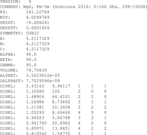
Figure 2. Descriptions of the input parameters of a Version 4 jcpds file [Citation11].
![Figure 2. Descriptions of the input parameters of a Version 4 jcpds file [Citation11].](/cms/asset/f983044f-1039-45f1-8305-7c3ba62c1510/ghpr_a_2187294_f0002_ob.jpg)
The thermal model used in Dioptas is a two-component thermal pressure model of the form
(1)
(1) where
is a modified pressure function of both volume and temperature, and
is the additional T-dependent thermal pressure given by
(2)
(2) where ΔT=(
298 K).
represents the 3rd-order Birch-Murnaghan function with temperature-dependent input parameters,
and
(3)
(3) where
(4)
(4) and
.
Importantly, Dioptas assumes a third order Birch-Murnaghan (B-M) EoS for the 298 K isotherm [Citation12], and it is, therefore, essential that the values of ,
and
in the jcpds files should be those for this form of EoS, and not those obtained from fits to other forms of EoS, such as the Vinet [Citation13] or AP2 [Citation14,Citation15]. While the parameters from these other EoSs can be very similar to those obtained by fitting the same data to a B-M EoS, this is not always the case, as will be shown later, and so refitting is typically required.
For temperatures other than 298 K, Dioptas calculates the thermal pressure correction that is applied to the component. Dioptas does this by first calculating the values of
,
and
(T) at that value of T via
(5)
(5)
(6)
(6)
(7)
(7) where
, and
,
and
are the zero-pressure volumetric thermal expansion, the zero-pressure bulk modulus, and the change in
with pressure, as determined at 298 K.
If the sample pressure is zero, then Dioptas calculates
(8)
(8) This is the volumetric expansion at P=0, and a comparison with experimental data provides a check of the correct values of
and
. Indeed, as will be shown below, the values of
and
in the jcpds file can be obtained by fitting the volumetric thermal expansion at zero pressure.
If the sample pressure is greater than zero, then Dioptas calculates the associated pressure using Equations (Equation1
(1)
(1) ) and (Equation2
(2)
(2) )
(9)
(9) and then numerically solves the 3rd order B-M EoS to determine
for the given values of
,
and
. We add a note of caution here that in cases where the second term of the right hand side of Equation (Equation2
(2)
(2) ) is greater than
, the EoS framework in Dioptas returns negative values for
. These negative pressures may then result in the calculated
being >1 when the numerical solution to the B-M EoS is performed. In practice, this behaviour typically occurs at low sample pressures and high temperatures and can result in a non-physical volume expansion following small increases in the pressure above 0 GPa. Fortunately, the affected PT space is limited in extent and for most applications can be ignored. For example, in the case of MgO, at 1500 K, with
K
and
GPa, the non-physical region is confined to
GPa. This anomaly is illustrated in (a) where the thermal expansion as calculated by Dioptas at
0.01 GPa is plotted alongside that calculated at P = 0 GPa. At temperatures above 600 K, the unit cell volume calculated at
0.01 GPa is clearly (and non-physically) larger than that calculated at 0 GPa at the same temperature.
Figure 3. The solid data points show (a) the 0 GPa volumetric thermal expansion, and (b) the 298 K isothermal compressibility of MgO, as calculated from the Sokolova et al. thermal EoS [Citation21]. The dashed line in (a) is the best fit to the thermal expansion using Equation (Equation8(8)
(8) ), while the dashed line in (b) is the best fit to the compressibility using a 3rd order Birch-Murnaghan EoS. The unfilled data points in (a) show the thermal expansion of MgO at 0.01 GPa, as calculated by Dioptas using the jcpds input file shown in . At a given temperature and this very low, but non-zero pressure, most of the MgO unit cell volumes calculated by Dioptas are greater than the associated volumes on the P=0 isobar, particularly at high temperatures. Effectively, Dioptas produces isotherms exhibiting expansion upon compression within a narrow pressure range. The reasons for this non-physical response are described in the main text.
![Figure 3. The solid data points show (a) the 0 GPa volumetric thermal expansion, and (b) the 298 K isothermal compressibility of MgO, as calculated from the Sokolova et al. thermal EoS [Citation21]. The dashed line in (a) is the best fit to the thermal expansion using Equation (Equation8(8) V=V0(1+αT(T)ΔT)=V0(1+α298ΔT+∂αT∂T|298ΔT2)(8) ), while the dashed line in (b) is the best fit to the compressibility using a 3rd order Birch-Murnaghan EoS. The unfilled data points in (a) show the thermal expansion of MgO at 0.01 GPa, as calculated by Dioptas using the jcpds input file shown in Figure 1. At a given temperature and this very low, but non-zero pressure, most of the MgO unit cell volumes calculated by Dioptas are greater than the associated volumes on the P=0 isobar, particularly at high temperatures. Effectively, Dioptas produces isotherms exhibiting expansion upon compression within a narrow pressure range. The reasons for this non-physical response are described in the main text.](/cms/asset/ee01f290-53ac-4d21-9af4-7ae997fb387f/ghpr_a_2187294_f0003_ob.jpg)
We can see that of the 6 thermal EoS parameters in the jcpds file, two ( and
) are obtained from a 3rd order B-M fit to the isothermal compression at
298 K, two
and
) are obtained from the zero pressure thermal expansion, and the final two (
, and
) are obtained from P-V-T data with
GPa and
K. This provides a straightforward route to obtaining optimum values of these parameters:
| (1) | Fit the isothermal compression at 298 K with a 3rd order B-M EoS and thereby determine values for | ||||
| (2) | Fit the ambient pressure volumetric expansion data using Equation 8, and thereby determine values for | ||||
| (3) | Using | ||||
3. Obtaining Dioptas thermal EoS parameters
3.1. MgO
To illustrate how the jcpds file for an individual material can be determined we give the example of the thermal EoS of MgO, a material commonly used as a high-PT calibrant and pressure transmitting medium and on which there have been many previous studies of its thermal-EoS [Citation16–21]. In obtaining optimum thermal EoS parameters for use in Dioptas we have chosen to reparameterise the existing thermal EoS of MgO recently published by Sokolova et al. which itself was optimised to fit a wealth of experimental data [Citation21].
Sokolova et al. also used a thermal pressure model for their EoS, but used Holzapfel's Adopted Polynomial (AP2) EoS to describe the room temperature compression [Citation14, Citation15], and an Einstein model for the high-temperature behaviour [Citation21]. This study was particularly useful in the current context as the authors provided Excel spreadsheets from which it was possible to straightforwardly calculate P or V at a given T for each material they studied despite the complexity of their thermodynamic model.
Firstly, we used Ref. [Citation21] to calculate the unit cell volume at 20 pressures from ambient up to 100 GPa at 298 K, and the resulting compression curve is shown in (b). Because Sokolova et al. used an AP2 EoS in their calculations, it is necessary to refit their compression data using a 3rd order B-M EoS rather than simply using their published AP2 values of ,
(160.3 GPa and 4.10, respectively) directly. Otherwise, direct use of the parameters may result in a significant discrepancy between the Dioptas output and the true EoS behaviour. The best fit to the compression curve using a B-M EoS gave
=161.11 GPa and
=4.010 and the resulting fit is shown in (b).
Next, to obtain values for and
we calculated the values of V at 21 different values of T from 298 to 1500 K at P=0.0001 GPa (atmospheric pressure) using Ref. [Citation21]. The calculated volumes are shown in (a), along with a fit using Equation (Equation8
(8)
(8) ). From this fit, the best fitting values of
and
are 3.502×10
K
and 7.753×10
K
, respectively.
Finally, in order to determine the optimum values of and
, we used Ref. [Citation21] to calculate P over a grid of 234 V-T values spanning 18 volumes from 74 to 53.6 Å
(which equates to a pressure range of approximately 0–100 GPa – see (b)) and 15 temperatures from 298 to 1500 K. Using the Solver minimisation routine in Excel, we then optimised the values of
and
while fixing the values of the other 4 parameters. The best fitting values were
GPa K
and 0.000193 K
, respectively. The final jcpds file is shown in .
The differences in calculated pressures, over a range of volumes and temperatures to ∼100 GPa and 1500 K, between the Sokolova thermal EoS and the best-fitting Dioptas EoS is shown in . The maximum differences, of ∼0.8 GPa, are seen at low pressures and high temperatures. The agreement between the Sokolova EoS and its reparameterisation for use in Dioptas is further illustrated in which shows three P-V isotherms at 298, 1000 and 1500 K, as calculated by the Sokolova EoS, and the Dioptas-calculated pressures at a number of different volumes at the same three temperatures. The agreement is excellent.
Figure 4. The differences in pressures calculated by the Sokolova et al. thermal EoS for MgO as a function of the unit cell volume and temperature, and the reparameterisation suitable for use in Dioptas via import of a jcpds file. The shown volume scale equates to a pressure range of approximately 0–100 GPa.
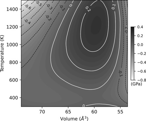
Figure 5. The 298, 1000 and 1500 K isotherms for MgO represented by the black dashed lines, as calculated using the thermal EoS of Sokolova et al. [Citation21]. The black square data points show a number of P-V data points along the three isotherms, as calculated by Dioptas using the jcpds file shown in .
![Figure 5. The 298, 1000 and 1500 K isotherms for MgO represented by the black dashed lines, as calculated using the thermal EoS of Sokolova et al. [Citation21]. The black square data points show a number of P-V data points along the three isotherms, as calculated by Dioptas using the jcpds file shown in Figure 1.](/cms/asset/eb5a79b2-545e-4c23-b935-1334fee0f9c1/ghpr_a_2187294_f0005_ob.jpg)
If the thermal EoS within Dioptas is required to cover a different, or larger, P-T range to that used here then it is straightforward to refit and optimise the parameters over different or more extended ranges of P-V-T data.
3.2. Neon
Ne is a commonly used pressure transmitting medium, and its compressibility and thermal EoS have therefore been the subject of several previous studies [Citation22–24]. In Ne, the values of ,
and
can again be obtained by fitting the room temperature isotherm with a 3rd order B-M EoS. Although solid Ne is only obtained above 4.7 GPa at 298 K [Citation22] a value for
can still be obtained from the B-M fit.
The fact that Ne is a gas at ambient conditions also means that the thermal expansion of solid-Ne is unknown above 298 K at atmospheric pressure and so the method described in the previous section for determining the values of and
cannot be used in this case. However, values for
and
can be obtained simultaneously with the values of
and
, by allowing all 4 parameters to vary when minimising the differences between the calculated pressures over a grid of V-T data.
In obtaining a suitable Ne jcpds input file for Dioptas we have chosen to reparameterise the thermal EoS of Ne published previously by Fei et al. [Citation23]. This used a thermal pressure model with both a Vinet and B-M 298 K isotherm, and a Mie–Grüneisen thermal pressure. Using this EoS we first calculated the 298 K compressibility and fitted it with a B-M EoS. As expected, we obtained values of 88.967 Å
/cell,
1.16 GPa and
8.23, exactly the same as those reported in Fei et al.'s 298 K B-M EoS [Citation23].
We then used the thermal EoS of Fei et al. to calculate the pressure at 144 V −T points covering a range of 54 to 24 Å, equivalent to a pressure range of 5–150 GPa, and 400 to 2000 K, and varied
,
,
and
simultaneously to minimise the difference between the Fei EoS and the Dioptas EoS. The optimised EoS parameters are given in , and the agreement between the two EoSs is illustrated in which shows the isotherms at 298, 1000 and 2000 K, as calculated by the Fei EoS, and the calculated volumes at a number of points along the 1000 and 2000 K isotherms, as calculated by Dioptas. The agreement is excellent.
3.3. hcp-Fe
The hcp phase of Fe (ϵ-Fe) is stable from 14 GPa up to at least 300 GPa at 298 K [Citation26]. While early studies suggested the existence of further high-temperature, high pressure phases, the most recent laser-heating studies of hcp-Fe suggest it is the only stable phase up to 377 GPa and 5700 K, conditions corresponding to Earth's inner core [Citation27].
Figure 6. The 298, 1000 and 2000 K isotherms for Ne, as calculated using the thermal EoS of Fei et al. [Citation23] are shown by the black dashed lines. The filled squares show a number of P-V data points along the 1000 and 2000 K isotherms, as calculated by Dioptas using the jcpds file input parameters for Ne given in .
![Figure 6. The 298, 1000 and 2000 K isotherms for Ne, as calculated using the thermal EoS of Fei et al. [Citation23] are shown by the black dashed lines. The filled squares show a number of P-V data points along the 1000 and 2000 K isotherms, as calculated by Dioptas using the jcpds file input parameters for Ne given in Table 1.](/cms/asset/2490f726-a8cd-42a4-ad6e-6c76c68bb840/ghpr_a_2187294_f0006_ob.jpg)
Table 1. The optimised thermal EoS parameters required for the jcpds files of various materials. is the unit cell volume for each material at ambient pressure, while the meanings of the other parameters are described in the main text.
Table 2. The as-published parameters for the room temperature AP2 EoS of Mo [Citation32], and the Vinet EoS of Au and Pt [Citation34].
In determining a Dioptas-suitable thermal EoS for hcp-Fe, we have chosen to reparameterise the recent EoS by Dorogokupets et al. [Citation25], which, as with results of Sokolova et al. [Citation21], was provided with spreadsheets so as to simplify the complex P-V-T calculations.
In hcp-Fe, the values of ,
and
were again obtained by fitting the room temperature isotherm with a 3rd order B-M EoS. Fitting P-V data at 5 GPa intervals between atmospheric pressure and 100 GPa, as calculated using the EoS of Dorogokupets et al. [Citation25], gave best fitting parameters of 22.642 Å
/atom (fixed), 150.475 GPa and 5.537, respectively.
Similar to the case of Ne, it is not possible to determine and
for hcp-Fe from the ambient pressure thermal expansion as this phase is stable only at high pressures. As with Ne therefore, values for
and
were obtained simultaneously with the values of
and
, by allowing all 4 parameters to vary when minimising the differences between the calculated pressures over a grid of V-T data.
We used the Dorogokupets et al. thermal EoS to calculate the pressure at 63 V-T points over a volume range of 17 to 21 Å, equivalent to a pressure range of 15–120 GPa, and over a temperature range of 500 to 3000 K, and varied
,
,
and
simultaneously to minimise the difference between the pressures calculated by the Dorogokupets EoS and the Dioptas EoS. The optimised values for the jcpds input parameters are given in , and the agreement between the two equations of state is illustrated in which shows the isotherms at 298, 1000, 2000 and 3000 K, as calculated by the Dorogokupets EoS, and the calculated volumes at a number of points along the 1000, 2000, and 3000 K isotherms as calculated by Dioptas. The agreement is excellent.
Figure 7. The 298, 1000, 2000 and 3000 K isotherms for hcp-Fe (ϵ-Fe), as calculated using the thermal EoS of Dorogokupets et al. [Citation25]. The filled squares show a number of P-V data points along the 1000, 2000 and 3000 K isotherms, as calculated by using the jcpds file input parameters for hcp-Fe given in .
![Figure 7. The 298, 1000, 2000 and 3000 K isotherms for hcp-Fe (ϵ-Fe), as calculated using the thermal EoS of Dorogokupets et al. [Citation25]. The filled squares show a number of P-V data points along the 1000, 2000 and 3000 K isotherms, as calculated by using the jcpds file input parameters for hcp-Fe given in Table 1.](/cms/asset/7e76aca8-ce51-4960-9ebd-163a66b29797/ghpr_a_2187294_f0007_ob.jpg)
Note that in calculating the positions of the diffraction peaks from hcp-Fe it is necessary to know the c/a ratio of the hexagonal structure. For hcp-Fe c/a is slightly pressure dependent [Citation28], something that the jcpds file format is unable to account for. In preparing a jcpds file for hcp-Fe, we have therefore fixed the c/a ratio at 1.6 [Citation28], and hence 2.5376 Å and
4.0601 Å at ambient pressure.
3.4. B2-KCl
KCl is often used as a pressure transmitting medium in high pressure laser heating experiments as it is soft, chemically inert, transparent in the near-infrared, and has a high melting temperature. At ambient conditions, KCl has the NaCl (B1) structure but transforms to the CsCl (B2) structure at ∼2 GPa, which is stable to 165 GPa at room temperature and also at high temperatures. Establishing a thermal EoS for KCl enables it to be used as a pressure calibrant at high pressures and temperatures. There have been two recent papers establishing a thermal EoS for KCl, by Dewaele et al. [Citation29] and Chidester et al. [Citation30]. Since the Dewaele EoS has been used by others in laser heating experiments we have chosen to parameterise that EoS here.
Dewaele et al. again used a thermal pressure model to fit their data, where the thermal pressure term could be approximated by
, where
is a constant. Hence:
(10)
(10) where
= 0.00244 GPa K
[Citation29].
In order to make a thermal EoS for B2-KCl suitable for use in Dioptas, we first calculated the 300 K compressibility using the Vinet EoS used by Dewaele et al. and then refitted it with a 3rd-order B-M EoS, giving optimised ,
and
values of 52.953 Å
, 24.606 GPa and 4.540, respectively. Note that rather than fixing the value of
at 54.5 Å
, the value reported by Dewaele et al., we optimised
simultaneously with those of
and
in order to improve the fit of the B-M EoS to the calculated compressibility at 300 K, which was otherwise poor.
We then used the thermal pressure model employed by Dewaele et al. to calculate the pressure at 112 V-T points over a volume range of 50 to 24 Å, equivalent to a pressure range of 2–130 GPa, and a temperature range of 500 to 3000 K. We then varied
,
,
and
simultaneously to minimise the difference between the pressures calculated by the Dewawele EoS and the Dioptas EoS.
Unsurprisingly, given the thermal EoS model used by Dewaele, the optimised values of ,
and
were all close to 0, while the optimised value of
was 8.944
K–1.
The optimised values for the parameters are given in , and the agreement between the two equations of state is illustrated in which shows the isotherms at 300, 2000 and 3000 K, as calculated from the thermal EoS parameters given by Dewaele et al., and the calculated volumes at a number of points along the same three isotherms as calculated by Dioptas. The agreement is, once again, excellent.
Figure 8. The 300, 2000 and 3000 K isotherms for the B2 phase of KCl, as calculated using the thermal EoS of Dewaele et al. [Citation29]. The filled squares show a number of data points along the same isotherms, as calculated by using the jcpds file input parameters for B2-KCl given in .
![Figure 8. The 300, 2000 and 3000 K isotherms for the B2 phase of KCl, as calculated using the thermal EoS of Dewaele et al. [Citation29]. The filled squares show a number of data points along the same isotherms, as calculated by using the jcpds file input parameters for B2-KCl given in Table 1.](/cms/asset/b3d391cd-1c6c-4823-afb2-149f607ba368/ghpr_a_2187294_f0008_ob.jpg)
3.5. Other common standards
We have repeated the analysis described above for a number of other materials whose thermal-EoS were parameterised by Sokolova et al. [Citation21], along with that of both the B1 and B2 phases of NaCl [Citation19,Citation23]. The resulting best-fitting parameters are given in , and the resulting jcpds files are provided in the Supplementary Material. We stress again that in all cases we are not developing new thermal EoSs for these materials but rather reparameterising existing thermal EoSs so that they are suitable for use with Dioptas after importing them via jcpds files.
Note that for NaCl-B1 we first attempted to reparameterise the thermal EoS of Dorogokuopets and Dewaele [Citation19], obtaining values of ,
,
and
simultaneously by fitting the isochore data given in Table 10 of Ref. [Citation19]. Unfortunately, the resulting values of
and
did not give a good fit to the known ambient pressure thermal expansion [Citation31]. Fortunately, the authors of Ref. [Citation19] were able to provide us with a greater number of P-V-T data points using their EoS, including the ambient pressure thermal expansion of NaCl.
and
could then be determined independently of
and
, with the resulting values giving a good fit to the thermal expansion at ambient pressure.
3.6. Room temperature ‘Primary’ pressure standards to 300 GPa
To help Dioptas users obtain accurate pressures in samples compressed to high pressures at room temperature, we provide jcpds input files for the room temperature EoS of 4 ‘primary’ pressure standards – Mo, Cu, Au and Pt – to 300 GPa. The first two of these were considered by an AIRAPT working group to establish an International Practical Pressure Scale [Citation32], while Au and Pt have recently been proposed as pressure calibrants at TPa pressures [Citation33,Citation34]. In each case we have taken the published room temperature equations of state for Mo (AP2 [Citation32]), Cu (3rd order Vinet [Citation33]), Au and Pt (2nd order Vinet [Citation34]), calculated their compression curves up to ∼300 GPa, and then refitted these using a B-M EoS. The resulting fits are illustrated in and the best fitting parameters are given in .
Figure 9. The room temperature equations of state of Mo, Cu, Au and Pt to 300 GPa. The data points show the calculated compressions using published AP2 (Mo) [Citation32], 3rd order Vinet (Cu) [Citation33], and 2nd order Vinet (Au and Pt) equations of state [Citation34]. The dashed lines through the data points are the best-fitting B-M equations of state, using the parameters listed in .
![Figure 9. The room temperature equations of state of Mo, Cu, Au and Pt to 300 GPa. The data points show the calculated compressions using published AP2 (Mo) [Citation32], 3rd order Vinet (Cu) [Citation33], and 2nd order Vinet (Au and Pt) equations of state [Citation34]. The dashed lines through the data points are the best-fitting B-M equations of state, using the parameters listed in Table 1.](/cms/asset/de084c2e-c986-4b1b-8aee-9bace5f5f95a/ghpr_a_2187294_f0009_ob.jpg)
In reparameterising these pressure standards, it is informative to compare the parameters originally published for the AP2 and Vinet equations of state for Mo, Au and Pt, with those obtained from the B-M fits. These are shown in , and highlight the very different values for and
required by the different EoS to produce almost identical compression curves (see ). This emphasises the importance of using the appropriate B-M values for
,
and
when using an existing EoS in Dioptas, rather than using the values obtained from fitting a different form of EoS. Interestingly, the parameters for the AP2/B-M fits for Mo in are much more similar than those obtained for the Vinet/B-M fits to Au and Pt, where the differences in the values of
and
in the two EoS are 30–150 times larger than the uncertainties obtained in the Vinet fits.
3.7. Tantalum thermal EoS to 2.3 TPa and 5000 K
Finally, we have reparametarised the very recently published thermal EoS of Ta, as determined to 2.3 TPa and 5000 K using a combination of ramp and shock compression data [Citation35]. This study greatly extends previous studies of the thermal EoS of tantalum, and, as the authors suggest, enables Ta to be used as a pressure calibrant in laser-heated static compression experiments which have recently been able to reach TPa pressures and thousands of degrees Kelvin. Reparameterising the published EoS was straightforward and followed the process described above. The values of and
were obtained by fitting the known ambient pressure thermal expansion, while the values of
and
were obtained by calculating the isothermal compression at 298 K to 2300 GPa using the 3rd order Vinet EoS employed by Gorman et al. [Citation35], and then refitting with a 2nd order B-M EoS. The 5 isotherms parameterised by Gorman et al. were then used to calculate a grid of 154 P-V points covering 0–2300 GPa and 298–5000 K from which the optimised values of
and
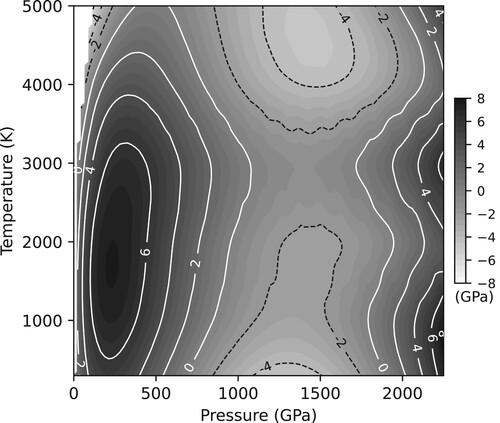
were obtained. The best fitting parameters are given in and the resulting jcpds file is provided in the Supplementary Material. The agreement between the Gorman and Dioptas equations of state is illustrated in which shows the difference in pressures as calculated from the thermal EoS parameters given by Gorman et al. [Citation35], and those calculated by Dioptas using the parameters in . The agreement is, once again, excellent. Indeed over the full 0–2300 GPa, 298–5000 K range, the maximum difference between the pressures calculated by two equations of state was only 8 GPa.
Figure 10. The differences in pressures between those calculated by the Gorman et al. thermal EoS for Ta, and those calculated by Dioptas using the parameters given in . Despite the very large P-T range (2300 GPa and 5000 K) the maximum difference between the two equations of state is only ∼8 GPa at 240 GPa and 1750 K. No contours are shown in the white area at low pressures (<100 GPa) and high temperatures (3300–5000 K) as Ta is in the liquid state at such conditions.
4. Limitations
While the results in the previous section show that the thermal pressure model within Dioptas is capable of reproducing the isotherms calculated by other thermal EoSs with a high degree of accuracy, there are a number of limitations. The jcpds files assume the Birch-Murnaghan formalism to describe the isothermal compression at 298 K. This is known to give a poorer fit to experimental data than other formalisms such as Vinet [Citation13] or AP2 [Citation14, Citation15], particularly at higher compressions, and it has been recommended that the BM EoS not be extrapolated beyond the data range to which it is fitted [Citation14].
Secondly, there may be no high-temperature thermal expansion data at 0 GPa from which to determine and
(as in the cases of Ne, hcp-Fe and B2-KCl above). However, as we have shown, these parameters can be optimsed from the high PT data simultaneously with
and
. In such cases, the values of
and
have no physical meaning.
Because of such limitations, we emphasise the importance of using the original EoS published in the literature for performing any final, in-depth analysis of new experimental data rather than the models and parameters presented here. The parameters given in are intended to enable the Dioptas user to closely reproduce the behaviour of published EoS models within Dioptas for the purposes of performing rapid analysis in real-time of experimental data collected on synchrotrons and x-ray free electron lasers. The insight gained from such feedback would facilitate users to make well-informed decisions during such experiments.
5. Conclusions
One of the advantages of Dioptas over other azimuthal integration software packages is its ability to read in jcpds files, and hence equation of states, for pressure calibration purposes. The jcpds file format allows thermal equations of state to be imported, but care must be taken to ensure that these are parameterised correctly. We have demonstrated how this can be achieved by reparameterising a number of existing equations of state, for a range of different materials, in the correct format for use in Dioptas. We have provided the required parameters in tabulated form, as well as the relevant jcpds files, and the spreadsheets used to obtain the parameters for each material. The jcpds files are also available for download with the most recent version of Dioptas available from https://github.com/Dioptas/Dioptas/releases.
Supplemental Material
Download MS Excel (59.4 KB)Supplemental Material
Download PDF (4.9 MB)Supplemental Material
Download Zip (15.4 KB)Acknowledgments
We would also like to thank Prof. Peter Dorogokupets for proving a spreadsheet to enable us to reproduce and supplement his thermal EoS calculations for B1-NaCl, as published in Ref. [Citation19].
Disclosure statement
No potential conflict of interest was reported by the author(s).
Correction Statement
This article was originally published with errors, which have now been corrected in the online version. Please see Correction (http://dx.doi.org/10.1080/08957959.2023.2225889)
Additional information
Funding
References
- Shimomura O, Takemura K, Fujihisa H, et al. Application of an imaging plate to high pressure x-ray study with a diamond anvil cell (invited). Rev Sci Instrum. 1992;63(1):967–973. DOI: 10.1063/1.1143793
- Nelmes RJ, Hatton PD, McMahon MI, et al. Angle-dispersive powder-diffraction techniques for crystal structure refinement at high pressure. Rev Sci Instrum. 1992;63(1):1039–1042. DOI: 10.1063/1.1143193
- Nelmes RJ, McMahon MI. High pressure powder diffraction on synchrotron sources. J Synchrotron Radiat. 1994;1(1):69–73. DOI: 10.1107/S0909049594006679
- Piltz RO, McMahon MI, Crain J, et al. An imaging plate system for high pressure powder diffraction: the data processing side. Rev Sci Instrum. 1992;63(1):700–703. DOI: 10.1063/1.1142641
- Hammersley AP, Svensson SO, Hanfland M, et al. Two-dimensional detector software: from real detector to idealised image or two-theta scan. High Press Res. 1996;14(4-6):235–248. DOI: 10.1080/08957959608201408
- Cervellino A, Giannini C, Guagliardi A, et al. Folding a two-dimensional powder diffraction image into a one-dimensional scan: a new procedure. J Appl Crystallogr. 2006;39(5):745–748. DOI: 10.1107/S0021889806026690
- Hinrichsen B, Dinnebier RE, Rajiv P, et al. Advances in data reduction of high pressure x-ray powder diffraction data from two-dimensional detectors: a case study of schafarzikite (FeSbsub2/subOsub4/sub). J Phys Condens Matter. 2006;18(25):S1021–S1037. DOI: 10.1088/0953-8984/18/25/S09
- Rodriguez-Navarro AB. XRD2DScan: new software for polycrystalline materials characterization using two-dimensional X-ray diffraction. J Appl Crystallogr. 2006;39(6):905–909. DOI:10.1107/S0021889806042488
- Kieffer J, Wright JP. PyFAI: a Python library for high performance azimuthal integration on GPU. Powder Diffr. 2013;28(S2):S339–S350. DOI: 10.1017/S0885715613000924
- Prescher C, Prakapenka VB. DIOPTAS: a program for reduction of two-dimensional X-ray diffraction data and data exploration. High Press Res. 2015;35(3):223–230. DOI: 10.1080/08957959.2015.1059835
- Merkel S. Example JCPDS file in the Version 4 format; 2006. Available from: https://merkel.texture.rocks/HPDiff/file_jcpds_4.php
- Birch F. Finite elastic strain of cubic crystals. Phys Rev. 1947;71(11):809–824. DOI: 10.1103/PhysRev.71.809
- Vinet P, Ferrante J, Rose JH, et al. Compressibility of solids. J Geophys Res Solid Earth. 1987;92(B9):9319–25. DOI: 10.1029/JB092iB09p09319
- Holzapfel WB. Equations of state for solids under strong compression. High Press Res. 1998;16(2):81–126. DOI:10.1080/08957959808200283
- Holzapfel WB. Equations of state for solids under strong compression. Z Krystallog. 2001;216(9):473–88. DOI:10.1524/zkri.216.9.473.20346
- Speziale S, Zha CS, Duffy TS, et al. Quasi-hydrostatic compression of magnesium oxide to 52 GPa: implications for the pressure-volume-temperature equation of state. J Geophys Res Solid Earth. 2001;106(B1):515–528. DOI: 10.1029/2000JB900318
- Fei Y, Li J, Hirose K, et al. A critical evaluation of pressure scales at high temperatures by in situ X-ray diffraction measurements. Phys Earth Planet Inter. 2004;143–144:515–526. DOI: 10.1016/j.pepi.2003.09.018
- Dorogokupets PI, Oganov AR. Ruby, metals, and MgO as alternative pressure scales: a semiempirical description of shock-wave, ultrasonic, x-ray, and thermochemical data at high temperatures and pressures. Phys Rev B. 2007;75(2):Article ID 024115. DOI: 10.1103/PhysRevB.75.024115
- Dorogokupets PI, Dewaele A. Equations of state of MgO, Au, Pt, NaCl-B1, and NaCl-B2: internally consistent high-temperature pressure scales. High Press Res. 2007;27(4):431–446. DOI: 10.1080/08957950701659700
- Sokolova TS, Dorogokupets PI, Litasov KD. Self-consistent pressure scales based on the equations of state for ruby, diamond, MgO, B2–NaCl, as well as Au, Pt, and other metals to 4 Mbar and 3000 K. Russ Geol Geophys. 2013;54(2):181–199. DOI: 10.1016/j.rgg.2013.01.005
- Sokolova TS, Dorogokupets PI, Dymshits AM, et al. Microsoft excel spreadsheets for calculation of PVT relations and thermodynamic properties from equations of state of MgO, diamond and nine metals as pressure markers in high pressure and high-temperature experiments. Comput Geosci. 2016;94:162–169. DOI: 10.1016/j.cageo.2016.06.002
- Finger LW, Hazen RM, Zou G, et al. Structure and compression of crystalline argon and neon at high pressure and room temperature. Appl Phys Lett. 1981;39(11):892–894. DOI: 10.1063/1.92597
- Fei Y, Ricolleau A, Frank M, et al. Toward an internally consistent pressure scale. Proc Natl Acad Sci USA. 2007;104(22):9182–9186. Available from: https://www.jstor.org/stable/25427827 DOI: 10.1073/pnas.0609013104
- Dewaele A, Datchi F, Loubeyre P, et al. High pressure-high temperature equations of state of neon and diamond. Phys Rev B. 2008;77(9):Article ID 094106. DOI: 10.1103/PhysRevB.77.094106
- Dorogokupets PI, Dymshits AM, Litasov KD, et al. Thermodynamics and equations of state of iron to 350 GPa and 6000 K. Sci Rep. 2017;7(1):Article ID 41863. DOI:10.1038/srep41863
- Mao HK, Wu Y, Chen LC, et al. Static compression of iron to 300 GPa and Fesub0.8/subNisub0.2/suballoy to 260 GPa: implications for composition of the core. J Geophys Res. 1990;95(B13):Article ID 21737. DOI:10.1029/jb095ib13p21737
- Tateno S, Hirose K, Ohishi Y, et al. The structure of iron in earth's inner core. Science. 2010;330(6002):359–361. DOI: 10.1126/science.1194662
- Dewaele A, Loubeyre P, Occelli F, et al. Quasihydrostatic equation of state of iron above 2 Mbar. Phys Rev Lett. 2006;97(21):Article ID 215504. DOI: 10.1103/PhysRevLett.97.215504
- Dewaele A, Belonoshko AB, Garbarino G, et al. High pressure–high-temperature equation of state of KCl and KBr. Phys Rev B. 2012;85(21):Article ID 214105. DOI: 10.1103/PhysRevB.85.214105
- Chidester BA, Thompson EC, Fischer RA, et al. Experimental thermal equation of state of B2-KCl. Phys Rev B. 2021;104(9):Article ID 094107. DOI: 10.1103/PhysRevB.104.094107
- Corish J, Catlow CRA, Jacobs PWM. The relationship between experimental and calculated point defect energies. J Physique Lett. 1981;42(15):369–372. DOI: 10.1051/jphyslet:019810042015036900
- Shen G, Wang Y, Dewaele A, et al. Toward an international practical pressure scale: a proposal for an IPPS ruby gauge (IPPS-Ruby2020). High Press Res. 2020;40(3):299–314. DOI:10.1080/08957959.2020.1791107
- Fratanduono DE, Smith RF, Ali SJ, et al. Probing the solid phase of noble metal copper at terapascal conditions. Phys Rev Lett. 2020;124:1Article ID 015701. DOI:10.1103/PhysRevLett.124.015701
- Fratanduono DE, Millot M, Braun DG, et al. Establishing gold and platinum standards to 1 terapascal using shockless compression. Science. 2021;372(6546):1063–1068. DOI:10.1126/science.abh0364
- Gorman MG, Wu CJ, Smith RF, et al. Ramp compression of tantalum to multiterapascal pressures: constraints of the thermal equation of state to 2.3 TPa and 5000 K. Phys Rev B. 2023;107(1):Article ID 014109. DOI: 10.1103/PhysRevB.107.014109