Intertemporal Risk-Return Relationship in Housing Markets

Abstract

We empirically investigate the intertemporal risk-return relationship in the U.S. housing market. Consistent with the theoretical predictions in Merton’s (1973) intertemporal capital asset pricing model (ICAPM), the national (regional) housing market displays a significantly positive relationship between its conditional variance (covariance) and capital gains. Results provide empirical support for housing showing that risk-averse agents require higher returns to reward higher risk in an intertemporal framework.

Keywords:

• Housing markets
• intertemporal capital asset pricing model
• risk-return relationship

Introduction

The trade-off between risk and return is a fundamental concept in finance. Among all asset classes, the risk-return relationship in housing is particularly worthy of attention. Bayer et al. (2010) emphasize the omission of the investment side of housing analysis is surprising since housing represents approximately two-thirds of the average American household’s financial portfolio. While a series of unconditional analyses in Cannon et al. (2006), Case et al. (2011), Beracha and Skiba (2013), and Beracha et al. (2018) have empirically supported the theoretical prediction of a positive risk-return trade-off in housing markets, little is known about whether the theoretical condition can hold over time. To bridge the gap, housing assets under a standard asset-pricing perspective, employing Merton’s (1973) intertemporal capital asset pricing model (ICAPM) are considered to relate housing returns to their price risk in a dynamic framework. The goal of this empirical research is to better understand whether risk-averse agents in housing would, as theory predicts, demand higher returns for bearing more risk over time.

While the existing housing literature has investigated the intertemporal relationship between “total risk” and return in regional markets (e.g., Dolde & Tirtiroglu, 1997; Han, 2013; Karoglou et al., 2013; Lee, 2017; Lin & Fuerst, 2014; Miles, 2008, 2011; Morley & Thomas, 2011, 2016; Willcocks, 2010; Zhou, 2016), much of the literature has not fully considered the underyling differences between aggregate and cross-sectional conditions in standard finance theory. The theoretical motivation of this article is that regional markets are submarkets within a nation; therefore, the preferred risk measure for regional markets is conditional covariance (i.e., systematic risk) rather than conditional variance (i.e., total risk) according to the cross-sectional condition in Merton (1973). Using this conceptualization for the empirical investigation, one can easily argue that the aggregate condition is best modeled at the national level, while the cross-sectional condition is preferably modeled at the regional level.

Systematic risk is important in housing since each regional market is affected by common macroeconomic factors such as interest rates. Concurrently, ripple effects across regional markets can also result in housing frenzies on a national scale (Chen & Chiang, 2019; Meen, 1999). As argued in Tsai (2014, 2015), regional housing markets can be connected with the national housing market. Therefore, consistent with much of the housing literature on unconditional analysis (e.g., Beracha et al., 2018; Beracha & Skiba, 2013; Cannon et al., 2006; Case et al., 2011), we proxy and measure systematic risk as the exposure to the broader housing market at the national level. Theoretically, both aggregate and cross-sectional conditions must hold and comply with each other. Accordingly, the present article has two goals. First, based on the aggregate condition, we assess whether the national housing market possesses a significantly positive relation between the conditional variance and return. Second, based on the cross-sectional condition, we examine whether there is a significantly positive trade-off between the conditional covariance and return across regional markets. By addressing these questions, new light is shed on the time-varying risk-return trade-off in housing markets.

The empirical analysis begins by examining the aggregate condition in the national housing market of the United States. Given that small sample inference is not suitable for modeling the conditional risk-return trade-off (Lundblad, 2007), to our knowledge this study is the first attempt to employ the historical national housing price index of Shiller (2015) and test the theoretically aggregate condition at the national level. Consistent with the theoretical prediction, results show a significantly positive risk-return trade-off between the conditional volatility and return using standard generalized autoregressive conditionally heteroskedastic in the mean (GARCH-M) models. The evidence of a significantly positive intertemporal relationship between the mean and variance in the broader housing market supports the fundamental prediction of the underlying asset pricing works of Merton (1973, 1980) and Campbell (1993).

Assessment of the cross-sectional condition for regional markets in the United States using the housing price index from the Federal Housing Finance Agency (FHFA) follows. Since small sample inference is not suitable for conditional risk-return modeling (e.g., Lundblad, 2007) and each of the regional housing markets has insufficient time-series observations, we follow Han (2013) and focus on nationwide cross-market analysis. Consistent with Han (2013), the conditional risk of each regional market is pooled into a panel data regression. The approach is similar to Han (2013), but Bayer et al. (2010) is also highlighted. Under this model, what matters for the risk premium of housing assets is their exposure to systematic risk. Therefore, the adopted risk measure is the conditional covariance predicted by bivariate GARCH modeling rather than the total risk generated by univariate GARCH modeling. In contrast to Han (2013), the empirical analysis of the cross-sectional condition in Merton’s (1973) ICAPM uncovers a significantly positive risk-return trade-off across metropolitan statistical areas (MSAs) in an intertemporal framework.

Consistent with most research on risk-return trade-off in housing markets, the empirical investigation in this study primarily focuses on the capital gain perspective. However, it should be noted that rental income (or implied rental income) accounts for a significant proportion of return on residential properties. To shed light on this less explored area, the housing price and rent index from Zillow is used to reassess the intertemporal risk-return trade-off across MSAs regarding capital appreciation and income, respectively. A positive intertemporal risk-return relation holds across MSAs for the capital gain, but not the rental yield. In the context of the rent saving of owner-occupiers, the insignificant risk-return trade-off across MSAs confirms the argument of local hedging incentives in the housing literature, which indicates households use current homes to hedge against future housing consumption risk (e.g., Cocco, 2000; Guo & Hardin, 2017; Han, 2008, 2010, 2013; Ortalo-Magne & Rady, 2002; Sinai & Souleles, 2005; Zhou, 2016), leading to weakening the positive risk-return trade-off.

The analyses in this study are an expansion of the unconditional works in Cannon et al. (2006), Case et al. (2011), Beracha and Skiba (2013), and Beracha et al. (2018). By treating housing as a single-period investment with static systematic risk, these works consistently show that housing markets that exhibit higher systematic risk are rewarded with higher capital gains. In this study, however, housing is a long-term investment and investors participate in housing markets for multiple years. Therefore, the expected risk and return will vary over time, due to changes in investment opportunities. The multiperiod conditional approach extends the unconditional literature by showing that the principle of a positive risk-return trade-off in the perspective of capital gain can hold not only across submarkets, but also over time. Though the principle of positive risk-return trade-off does not hold empirically across MSAs in the setting of rental yield, the findings point to the need for future studies to revisit the empirical asset pricing work in housing, employing the return comprising the income component.

Finally, this study extends Han’s (2013) seminal work by considering the cross-sectional condition in Merton’s (1973) ICAPM. This article complements Han’s (2013) solution to the puzzle of a negative risk-return trade-off by focusing on the modeling differences of a market clearing condition between regional and national housing markets in line with Merton’s (1973) theoretical work. Overall, the empirical evidence using aggregate and cross-sectional analyses consistently indicates that housing markets obey the intertemporal mean-variance efficiency from the capital gain perspective.

Literature Review

Risk-aversion is a fundamental concept in finance: risk-averse agents require additional rewards to bear additional risk. Since the canonical capital asset pricing model (CAPM) of Sharpe (1964) and Lintner (1965) and the arbitrage pricing theory of Ross (1976), the finance literature has empirically established that market-wide risk is a key determinant of variation in security prices. Accordingly, systematic risk cannot be diversified, prompting risk-averse investors to demand compensation for this risk. Therefore, an asset’s sensitivity to market risk is positively associated with the expected returns of the asset. This positive relationship between reward and systematic risk is an important determinant of the cross-sectional returns in residential real estate markets as well (Beracha et al., 2018; Beracha & Skiba, 2013; Cannon et al., 2006; Case et al., 2011).

Against the backdrop of the CAPM, Merton (1973) derives a conditional two-factor model, comprising factors for systematic and hedging risk, and which considers investors’ future consumption and investment opportunities. Unlike the CAPM, the risk-return relationship in the ICAPM is time-varying and, since the supply of available assets change, so too does the conditional covariance of returns on those assets. The intertemporal risk-return trade-off in Merton (1973) has been examined empirically in both the equity and housing literatures, with mixed results.

The debate over the validity of the ICAPM in describing the risk-return trade-off can be traced to Campbell (1987) and French et al. (1987), who find conflicting evidence regarding the sign of a risk-return relationship in equity markets. French et al. (1987) find an insignificantly positive risk-return trade-off via GARCH modeling, while Campbell (1987) finds a statistically significant negative relationship using instrumental variables. One of the pioneering studies by Baillie and DeGennaro (1990) shows that if one sets the conditional distribution of the stock return shock from the Student’s t to the normal distribution, the risk-return trade-off becomes significantly positive. Considering the empirical contradictions against the theoretical prediction, more recent equity literature emphasizes the development of better identification methodologies for detecting a positive risk-return relationship: focusing on sample size (e.g., Lundblad, 2007), the measurement of expected return (e.g., Pastor et al., 2008), measurement of conditional variance (e.g., Ghysels et al., 2005; Jiang & Lee, 2014), regime-switching models (e.g., Ghysels et al., 2014; Liu, 2017; Nyberg, 2012; Salvador et al., 2014; Yu & Yuan, 2011), and the inclusion of a hedging factor (e.g., Guo & Whitelaw, 2006; Rossi & Timmermann, 2015; Scruggs, 1998).

More recent research revisits the conditional trade-off between risk and return in the housing asset class (e.g., Dolde & Tirtiroglu, 1997; Han, 2013; Karoglou et al., 2013; Lee, 2017; Lin & Fuerst, 2014; Miles, 2008, 2011; Morley & Thomas, 2011, 2016; Willcocks, 2010; Zhou, 2016). However, empirical results across studies and geography are inconsistent. For example, at the state level, Miles (2008) finds a significantly positive risk-return relationship in Georgia, but a significantly negative relationship in Nebraska. At the city level, Karoglou et al. (2013) find a significantly positive risk-return relationship in Portland, but a significantly negative relationship in Chicago.

While the examination of the intertemporal risk-return relationship in the equity market attracts scant attention, it garners even less in the housing literature. A majority of the housing literature focuses on the application of GARCH-M models to test the theoretically aggregate condition for each of the regional markets, respectively. Han (2013) provides a link between these approaches, however, by considering the dual financial-asset and consumption-hedge role of housing. Han (2013) argues that households use their current home to hedge against future housing consumption risk, so they opt to accept a lower return to compensate for this risk. Han (2013) empirically finds that after controlling the impact of consumption hedge, the negative sign of the intertemporal risk-return relationship across U.S. housing markets becomes positive.

However, Han (2013) does not consider the cross-sectional condition in Merton’s (1973) ICAPM, while testing the risk-return puzzle in regional housing markets by using the aggregate condition. When mapping Merton’s (1973) theory to empirical data, the first step is to test whether there is a positive time-varying risk-return trade-off in housing markets, with the next logical question being to identify the hedging factor. This study focuses on the former by testing the theory more closely to the spirit of Merton (1973) and is, therefore, to our knowledge the first attempt to incorporate a full picture of standard finance theory into housing analysis. This research complements Han’s (2013) solution to the negative risk-return puzzle in housing by considering the modeling differences between aggregate and cross-sectional conditions in Merton’s (1973) ICAPM. The initial analysis reexamines the intertemporal risk-return trade-off relationship across U.S. housing markets as in Han (2013). This study differs, however, in recognizing that regional housing markets are couched within the broader national housing market. In doing so, we explicitly model the risk-return trade-off at the regional level as a function of systematic risk, rather than total risk per the extant research.

Building on the unconditional work of Cannon et al. (2006), Case et al. (2011), Beracha and Skiba (2013), and Beracha et al. (2018), regional housing returns to systematic risk at the national level are related, and the market risk-adjusted sensitivity of the changes in regional housing prices to movements in the aggregate housing market is assessed. While unconditional methods establish that the U.S. metropolitan real estate market conforms with the standard asset pricing hypothesis that higher systematic risk is rewarded with higher return on average, little is known about whether this condition can hold over time. Motivated by Merton’s (1973) ICAPM, this research extends the literature by examining whether the principle of a positive risk-return trade-off can hold intertemporally in housing markets.

Theory

This study is the first, or one of the first, to consider the differences between aggregate and cross-sectional conditions in the context of housing markets. Consequently, the literature for this topic in the housing setting is underdeveloped. This section therefore commences by providing a theoretical motivation through the ICAPM lens, before extending its implications to the housing market.

ICAPM

Assuming the existence of risk-averse representative agents, the cross-sectional condition of Merton (1973) indicates that the excess return of an asset i ($r_{i,t+1}$) is a linear function of its conditional covariance with the aggregate market (${\sigma }_{im,t+1}$) and covariance with investment opportunities (${\sigma }_{is,t+1}$): (1) $$E_t\left[r_{i,t+1}\right]=\left(\frac{-J_{ww}W}{J_w}\right){\sigma }_{im,t+1|t}+\left(\frac{-J_{ws}W}{J_w}\right){\sigma }_{is,t+1|t},$$(1) where W(t) is individual wealth, S(t) is a variable describing the state of investment opportunities in the economy, and J (W, S, t) represents the investor’s indirect utility function. Subscripts of J denote partial derivatives. $(-J_{ww}W/J_w)$ is the related risk aversion and is assumed to be positive, indicating a positive risk-return trade-off for risk-averse agents.

An aggregate market condition is formed by summing Equation (1)(1) $$E_t\left[r_{i,t+1}\right]=\left(\frac{-J_{ww}W}{J_w}\right){\sigma }_{im,t+1|t}+\left(\frac{-J_{ws}W}{J_w}\right){\sigma }_{is,t+1|t},$$(1) for each of the regional markets and multiplying by its corresponding market weights ($w_i$): (2) $$E_t\left[\sum _1^n{w}_i\left(r_{i,t+1}\right)\right]=\sum _1^n{w}_i\left[\left(\frac{-J_{ww}W}{J_w}\right){\sigma }_{im,t+1|t}+\left(\frac{-J_{ws}W}{J_w}\right){\sigma }_{is,t+1|t}\right],$$(2) where$\mathrm{ }{r}_{m,t+1}\equiv {\sum }_1^n{w}_i\left(r_{i,t+1}\right),\mathrm{ }{\mathrm{ }\sigma }_{m,t+1|t}^2\equiv {\sum }_1^n{w}_i{\sigma }_{im,t+1|t}\mathrm{ }$ and ${\sigma }_{ms,t+1|t}\equiv {\sum }_1^n{w}_i{\sigma }_{is,t+1|t}.$ (3) $$E_t\left[r_{m,t+1}\right]=\left(\frac{-J_{ww}W}{J_w}\right){\sigma }_{m,t+1|t}^2+\left(\frac{-J_{ws}W}{J_w}\right){\sigma }_{ms,t+1|t}.$$(3)

Equation (3)(3) $$E_t\left[r_{m,t+1}\right]=\left(\frac{-J_{ww}W}{J_w}\right){\sigma }_{m,t+1|t}^2+\left(\frac{-J_{ws}W}{J_w}\right){\sigma }_{ms,t+1|t}.$$(3) shows that the conditional market risk premium is a linear function of its conditional variance and covariance with investment opportunities (the hedging component). If we assume that a regional housing market is part of a national market, then the progression from Equations (1)(1) $$E_t\left[r_{i,t+1}\right]=\left(\frac{-J_{ww}W}{J_w}\right){\sigma }_{im,t+1|t}+\left(\frac{-J_{ws}W}{J_w}\right){\sigma }_{is,t+1|t},$$(1) to (3)(3) $$E_t\left[r_{m,t+1}\right]=\left(\frac{-J_{ww}W}{J_w}\right){\sigma }_{m,t+1|t}^2+\left(\frac{-J_{ws}W}{J_w}\right){\sigma }_{ms,t+1|t}.$$(3) quantitatively proves that the cross-sectional condition is the corresponding market clearing condition for regional markets.

Further, as is well documented in the equity literature (e.g., Frazier & Liu, 2016; Ghysels et al., 2005, 2014; Guo & Whitelaw, 2006; Jiang & Lee, 2014; Liu, 2017; Lundblad, 2007; Nyberg, 2012; Rossi & Timmermann, 2015; Salvador et al., 2014; Scruggs, 1998; Wang, 2005; Yu & Yuan, 2011), the aggregate market condition in Merton (1973) is a unique phenomenon that is typically investigated at the national level. If regional housing markets are part of the national market, it follows, in theory, that systematic risk is a more suitable pricing factor for regional markets.

The general model can be reduced to a restricted form, assuming that the investment opportunity set is time-invariant or that the representative market participant has log utility (e.g., Lundblad, 2007). While both assumptions can be extreme, Merton (1980) contends that the general intertemporal equilibrium risk-return trade-off can still be reasonably approximated. Therefore, much of the literature (e.g., Bali, 2008; Frazier & Liu, 2016; Ghysels et al., 2005; Han, 2013; Lundblad, 2007; Nyberg, 2012; Pastor et al., 2008; Yu & Yuan, 2011) tests the intertemporal risk-return relationship in the reduced form of the ICAPM. The theoretical condition in Equations (1)(1) $$E_t\left[r_{i,t+1}\right]=\left(\frac{-J_{ww}W}{J_w}\right){\sigma }_{im,t+1|t}+\left(\frac{-J_{ws}W}{J_w}\right){\sigma }_{is,t+1|t},$$(1) and (3)(3) $$E_t\left[r_{m,t+1}\right]=\left(\frac{-J_{ww}W}{J_w}\right){\sigma }_{m,t+1|t}^2+\left(\frac{-J_{ws}W}{J_w}\right){\sigma }_{ms,t+1|t}.$$(3) can be further specified as below: (4) $$E_t\left[r_{i,t+1}\right]=\left(\frac{-J_{ww}W}{J_w}\right){\sigma }_{im,t+1|t},$$(4) (5) $$E_t\left[r_{m,t+1}\right]=\left(\frac{-J_{ww}W}{J_w}\right){\sigma }_{m,t+1|t}^2.$$(5)

Housing Theory

Unlike financial assets, housing serves a dual role, as an investment vehicle and a consumption good. Housing offers service and utility, simultaneously representing a store of value. Sinai and Souleles (2005) find that homeownership can hedge against fluctuations in housing costs since houses can pay off the ex-post spot rent. Guo and Hardin (2017) further document that in the long-run, the ability to hedge housing expenditures as a homeowner allows households to increase nonhousing expenditures. A body of literature suggests that owning a property allows households to hedge against housing consumption risk in the future (e.g., Cocco, 2000; Guo & Hardin, 2017; Han, 2008, 2010, 2013; Ortalo-Magne & Rady, 2002; Sinai & Souleles, 2005; Zhou, 2016).

From the investment side of standard asset pricing theory, higher risk of current home investment will require a higher compensation of return (a financial risk effect). As argued by Yang et al. (2018), household portfolio decisions are linked to expected housing development and financial market dynamics. However, homeowners also face risk in the local markets within which they reside. From the consumption perspective in housing theory, local hedging incentives against future consumption risk by owning a home would require a lower return to compensate for consumption risk (a consumption hedge effect). To reconcile the two theories, Han (2013) argues that the predicted risk-return relation of ICAPM in the context of housing can be uncertain (either positive, insignificant, or negative) depending on the competing strength between the financial risk and consumption hedge effects.

This research complements Han’s (2013) work in two ways. First, although Han (2013) empirically examines the intertemporal risk-return trade-off across U.S. regional markets based on the aggregate condition in Merton’s (1973) ICAPM, the appropriate setting to test the theoretical prediction in ICAPM should be the cross-sectional condition for regional housing markets. In line with the unconditional risk-return analyses in the housing literature by Cannon et al. (2006), Case et al. (2011), Beracha and Skiba (2013), and Beracha et al. (2018), systematic risk is adopted as a pricing factor for regional markets rather than total risk.

Second, Han’s (2013) empirical work, examining intertemporal risk-return trade-off across U.S. regional markets, is conducted based on a capital gain perspective. However, according to Jorda et al. (2019), capital gains, on average, account for only 23.27% in total return in real terms, based on annual data covering 16 countries from 1870 to 2015. Given that rental income comprises a significant proportion of total return, Han (2013) is expanded by specifically investigating the intertemporal risk-return trade-off in regional markets, on considering both income and capital appreciation. Rent saving, in the case of owner-occupiers, is fundamentally linked to the consumption demand for housing. It therefore follows that on examining the effect of rental yield, the consumption hedge effect is more likely to dominate the financial risk effect, leading to an insignificant or negative risk-return trade-off in regional markets.

ICAPM Aggregate Analysis

In this section, the intertemporal relationship between the market return and its conditional variance, based on the aggregate condition in Merton’s (1973) ICAPM is examined. Consistent with the equity and housing literature,¹ we consider the market portfolio at the “national” level, and proxy the U.S. housing market portfolio using a national housing price index, to test the aggregate condition.

Data

Two U.S. housing price indices are used in this section: the FHFA and Shiller (2015). While the FHFA house price index comprises the most comprehensive cross-sectional and time-series set of quality-adjusted house price indices available in the United States (Case et al., 2011), the Shiller (2015) national housing price index contains the longest time-series, which traces back to 1890. To draw on the relative strengths of both indices, this study applies the two sets of the national housing price indices. Given that the national home price index in Shiller (2015) contains more time-series observations and is more suitable for the application of GARCH-M models, this section focuses on the result of this index.²

The FHFA and Shiller (2015) house price indices are weighted repeat-sales indices, capturing average price changes in repeat sales or refinancing on the same single-family property. Though the two indices are frequently used for U.S.-based research, the common limitations of using the repeat-sales index should also be acknowledged.³ First, the repeat-sales method involves several assumptions, as summarized in Epley (2016). An example of this is to assume that the quality of the individual properties remains constant over time. Yet a dwelling sold at two different sale dates is not necessarily identical due to depreciation and renovation. Second, the repeat sales method is not immune to selection bias since it is constructed based on the properties that have sold more than once during the sample period and, thus, can be a nonrepresentative sample for the objects of interest (Guo et al., 2014). Third, a repeat sales dataset can be augmented with appraisals. Appraisers may rely on past information, introducing bias and smoothing in valuations (Geltner et al., 2003).

Following the majority of the housing literature (e.g., Beracha & Skiba, 2013; Beracha et al., 2018; Cannon et al., 2006; Case et al., 2011; Cotter et al., 2015; Dolde & Tirtiroglu, 1997; Han, 2013; Karoglou et al., 2013; Lee, 2017; Lin & Fuerst, 2014; Miles, 2008, 2011; Morley & Thomas, 2011; Zhou, 2016), we assess the way expected housing returns interact with risk from a capital gain perspective.⁴ Consistent with the recent housing literature (e.g., Beracha et al., 2018; Cotter et al., 2015; Han, 2013; Zhou, 2016), housing returns are measured in real terms, using the real national home price index in Shiller (2015) as the proxy for the performance of the aggregate U.S. market with returns measured as the first difference of the natural logarithm. Further, since the univariate GARCH-M analysis is known to be sensitive to sample size, the historical U.S. housing market record from January 1954 to October 2019 is used to maximize the time series length.⁵

Table 1 presents the summary statistics of monthly housing returns. Compared with the documented sample size (from 48 to 264 observations) used in previous work within the United States (e.g., Dolde & Tirtiroglu, 1997; Han, 2013; Karoglou et al., 2013; Miles, 2008), the national home price index in Shiller (2015) provides sufficient observations to run GARCH-M models.

Table 1. Summary statistics of monthly housing returns.

	Mean (%)	SD (%)	Min (%)	Max (%)	Obs.
Housing return	0.06	0.55	−2.54	2.12	789

Notes. The returns are calculated as: $R_t=ln (P_t/P_{t-1}$) where $P_t$ is the price index at time t, from 1954: M1 to 2019: M10. The real U.S. national home price index in Shiller (2015) is used for the construction of the housing return.

Methodology

Econometric modeling investigating the aggregate condition in ICAPM lends itself to the GARCH-M methodology, as follows:⁶ (6) $$R_{m,t}={\alpha }_0+{\alpha }_M{\sigma }_{M,t}^2+{\epsilon }_t,$$(6) where$R_{m,t}$ is the real market return and ${\epsilon }_t$ is the error term of mean zero with conditional variance ${\sigma }_{M,t}^2.$ The assumption of risk-averse agents implies that ${\alpha }_M>0.$ Following Lanne and Saikkonen (2006), ${\alpha }_0$ is restricted to be zero since 1) the intercept shall equal zero in theory and 2) the unnecessary intercept in the GARCH-M model leads to serious lack of power in the standard Wald test on the mean effect$.$

Without loss of generality for the variance equation, different standardized variance component specifications for the evolution of conditional volatility are incorporated: GARCH (Bollerslev, 1986), Threshold GARCH (TGARCH) (Zakoian, 1994), Exponential GARCH (EGARCH) (Nelson, 1991), and Component GARCH (CGARCH) (Engle & Lee, 1999): (7) $$\mathrm{GARCH}\left(1,1\right):\mathrm{ }{\sigma }_{M,t}^2={\delta }_0+{\delta }_1{\epsilon }_{t-1}^2+{\delta }_2{\sigma }_{M,t-1}^2,$$(7) (8) $$\mathrm{TGARCH}(1,1):{\sigma }_{M,t}^2={\delta }_0+{\delta }_1{\epsilon }_{t-1}^2+{\delta }_2{\sigma }_{M,t-1}^2+{\delta }_3{D}_{t-1}{\epsilon }_{t-1}^2,$$(8) (9) $$\mathrm{EGARCH}(1,1):\ln \left({\sigma }_{M,t}^2\right)={\delta }_0+{\delta }_1\left(\left|\frac{{\epsilon }_{t-1}}{{\sigma }_{M,t-1}}\right|\right)+{\delta }_2\ln \left({\sigma }_{M,t-1}^2\right)+{\mathrm{ }\delta }_3\left(\frac{{\epsilon }_{t-1}}{{\sigma }_{M,t-1}}\right),$$(9) where $D_{t-1}$ is a dummy variable taking the value of one when ${\epsilon }_{t-1}^{}$ is negative and zero otherwise. The GARCH model suggests a symmetric response in conditional volatility after return innovation, while the ${\delta }_3$ in the TGARCH and EGARCH allows asymmetric shocks on conditional volatility (Engle & Ng, 1993). The variance equation of CGARCH takes a different form, allowing the volatility to be decomposed into permanent ($q_t$) and transitory (${\sigma }_{M,t}^2-q_t$): (10) $$\mathrm{CGARCH}(1,1):{\mathrm{ }q}_t={\delta }_0+{\delta }_1\left(q_t-{\delta }_0\right)+{\delta }_2\left({{\epsilon }_{t-1}^2-\sigma }_{M,t-1}^2\right),$$(10) (11) $${\sigma }_{M,t}^2-q_t={\delta }_3\left({\epsilon }_{t-1}^2-q_{t-1}\right)+{\delta }_4\left({\sigma }_{M,t-1}^2-q_{t-1}\right).$$(11)

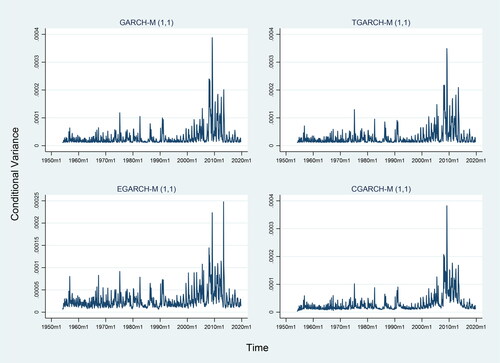
Using the return information, the predicted conditional variance using the GARCH-M models based on Equations (7)–(11) is derived. Figure 1 plots the predicted conditional variance from the baseline models with the normal error distribution. The conditional heteroskedasticity of variance is obvious in Figure 1. Several distinct periods of high market volatility (“volatility clusters”) are visible. As expected, the housing market was more volatile during the recent global financial crisis (GFC). Large volatility shocks seem to decay within a year across the entire sample.

Figure 1. Conditional variance generated by GARCH-M models.

Note. This figure plots the conditional variance generated by GARCH-M models over the period February 1954 to October 2019.

Empirical Results

As GARCH-M model results can be sensitive to volatility specification (Glosten et al., 1993), four common GARCH-M variants (GARCH-M, Threshold GARCH-M, Exponential GARCH-M and Component GARCH-M) are used for robustness. Since Baillie and DeGennaro (1990) also show that results can be sensitive to assumptions about the distribution of error terms, we further consider three variants of error distribution for each model (normal, Student’s t, and generalized). In total, 12 GARCH-M models are used with the results reported in Table 2.

Table 2. GARCH-M results at the national level.

	Model specifications		${\alpha }_M$ (risk-return)	${\delta }_0$×10^−6	${\delta }_1$	${\delta }_2$	${\delta }_3$	${\delta }_4$	Log likelihood (R-squared)
(1)	Panel A: GARCH(1,1)-M	Normal	17.81*** (6.27)	10.10*** (1.20)	0.50*** (0.08)	0.12* (0.07)			3111.05 (−0.05)
(2)		Student’s t	16.99*** (6.28)	9.82*** (1.39)	0.52*** (0.09)	0.13* (0.08)			3111.85 (−0.05)
(3)		Generalized	17.80*** (6.33)	10.10*** (1.26)	0.50*** (0.08)	0.12* (0.07)			3111.05 (−0.05)
(4)	Panel B: TGARCH(1,1)-M	Normal	21.49*** (6.36)	10.10*** (1.21)	0.57*** (0.12)	0.12* (0.07)	−0.13 (0.13)		3111.59 (−0.04)
(5)		Student’s t	22.02*** (6.34)	9.83*** (1.45)	0.63*** (0.15)	0.12 (0.08)	−0.19 (0.15)		3112.77 (−0.04)
(6)		Generalized	21.66*** (6.39)	10.10*** (1.31)	0.58*** (0.13)	0.12* (0.07)	−0.14 (0.14)		3111.63 (−0.04)
(7)	Panel C: EGARCH(1,1)-M	Normal	22.46*** (7.00)	−5.04 × 10^6*** (0.75 × 10^6)	0.74*** (0.08)	0.58*** (0.07)	0.02 (0.05)		3104.28 (−0.02)
(8)		Student’s t	23.12*** (6.95)	−4.68 × 10^6*** (0.84 × 10^6)	0.75*** (0.09)	0.62*** (0.08)	0.05 (0.06)		3105.77 (−0.01)
(9)		Generalized	22.73*** (7.03)	−4.97 × 10^6*** (0.80 × 10^6)	0.74*** (0.08)	0.59*** (0.07)	0.03 (0.05)		3104.39 (−0.02)
(10)	Panel D: CGARCH(1,1)-M	Normal	18.41*** (6.65)	23.40*** (4.66)	0.94*** (0.02)	0.08* (0.04)	0.37*** (0.08)	−0.16 (0.14)	3127.83 (−0.05)
(11)		Student’s t	18.41*** (6.72)	23.40*** (4.89)	0.94*** (0.02)	0.08* (0.04)	0.37*** (0.08)	−0.16 (0.14)	3127.83 (−0.05)
(12)		Generalized	19.42*** (6.74)	22.90*** (3.75)	0.94*** (0.02)	0.08** (0.04)	0.36*** (0.07)	−0.18 (0.13)	3129.29 (−0.05)

Notes. The table presents coefficient estimates based on Equations (6)–(11) for different versions of GARCH-M models. Numbers in parentheses denote the corresponding standard errors for the coefficients. ***, **, and * denote significance levels at 1%, 5%, and 10%, respectively.

All the GARCH-M models consistently show a significantly positive risk-return relationship based on the coefficient estimate of ${ \alpha }_M,$ significant at the 1% level across all 12 models.⁷ The magnitude of the risk-aversion is reasonable, and similar to the U.S. equity evidence in Scruggs (1998). Overall, these results are robust to alternate specifications and are not affected by error term assumptions. The consistency of the results supports the conclusion of a significantly positive intertemporal risk-return trade-off in the U.S. national housing market.

Implications

To better understand the implications of this approach and its success in examining the intertemporal risk-return relationship in housing, the present results are compared to those in the equity literature. Since the pioneering work by French et al. (1987), which finds conflicting evidence regarding the sign of risk-return relationship in equity markets, subsequent literature has recognized the empirical difficulty of documenting theoretical predictions via GARCH-M models, and devoted much effort to developing better identification methodologies (e.g., Frazier & Liu, 2016; Ghysels et al., 2005; Guo & Whitelaw, 2006; Jiang & Lee, 2014; Liu, 2017; Lundblad, 2007; Nyberg, 2012; Pastor et al., 2008; Rossi & Timmermann, 2015; Salvador et al., 2014; Scruggs, 1998; Yu & Yuan, 2011).

Few studies, however, consider the application of a different market proxy. The aggregate market proxy should ideally cover a wide range of capital assets such as financial assets, real estate, government bonds, consumer durables, and human capital (Fama & French, 2004). As highlighted in Roll’s (1977) critique, the composition of a true market portfolio composed of all assets is elusive and unmeasurable. Hence, the present study follows the unconditional risk-return analyses in the housing literature – namely Cannon et al. (2006), Case et al. (2011), Beracha and Skiba (2013) and Beracha et al. (2018) – while considering an alternative to the aggregate wealth portfolio focusing on housing assets. While it is recognized that 1) the national housing price index is not the ideal “market portfolio” and 2) ICAPM in Merton (1973) is not a perfect asset-pricing model, the ICAPM remains one of most fundamental natural starting points for understanding assets’ intertemporal risk-return features.

A weakness to most previous approaches in the finance risk is that the theoretically positive intertemporal risk-return relationship cannot robustly hold in equities across different types of GARCH-M models. In this study, the empirical results of the intertemporal risk-return relationship in housing are surprisingly positive, irrespective of volatility specifications in all 12 versions of the standard GARCH-M model. The possible explanation for this success is that, unlike financial assets, housing is durable, serving as a long-term investment that provides a stream of services. The decision-making process for homebuyers is therefore known to be forward-looking (Paciorek, 2013). Such a factor indicates that the intertemporal risk-return relationship in housing can be more pronounced and, thus, more successfully detected by GARCH-M models.

ICAPM Cross-Sectional Analysis

Han (2013) documents a negative intertemporal risk-return trade-off across U.S. regional markets through a panel data analysis. This section revisits this analysis, albeit by focusing on the cross-sectional condition of Merton’s (1973) ICAPM.

Data

The data used for the following is the real housing return, at the regional and national levels. Consistent with Case et al. (2011), Han (2013), Glaeser et al. (2014), Cotter et al. (2015), and Beracha et al. (2018), we employ the all-transaction housing price index from FHFA to construct housing returns by using the first difference of the natural logarithm. Application is focused on the FHFA all-transaction index over the purchase-only index since, first, the results can be compared more directly against the prior literature (e.g., Han, 2013) and, second, the purchase-only index begins in 1991 with fewer metropolitan areas. All of the housing price indices are deflated by the net-of-shelter consumer price index published by the Bureau of Labor Statistics (BLS).

Following the approach taken in the related housing literature, the proposed sample period starts from 1985:Q1 to maximize the representation of MSAs.⁸ The sample period ends in 2007:Q2 to avoid the possible confounding effects of the recent GFC, as indicated in Han (2013) and Loutskina and Strahan (2015). Excluding the GFC period from our sample allows a more direct comparison of the results against the conditional work of Han (2013) and the unconditional work in Cannon et al. (2006) and Case et al. (2011). After dropping some of the regional markets that contain missing variables, the sample contains 206 MSAs. Table 3 displays the related summary statistics of eight MSAs.⁹

Table 3. Summary statistics of quarterly housing returns.

	Mean (%)	SD (%)	Min (%)	Max (%)	Obs.
Miami	1.11	2.03	−5.56	5.82	89
Chicago	0.79	0.98	−1.84	3.54	89
Portland	0.73	2.06	−4.77	5.53	89
San Jose	1.22	2.52	−4.88	7.06	89
Cincinnati	0.33	0.75	−1.94	2.68	89
New York	0.96	2.15	−4.26	7.44	89
Los Angeles	1.16	2.56	−4.90	9.60	89
San Francisco	1.26	2.28	−4.49	6.31	89

Notes. We use the deflated FHFA housing price index for the construction of the housing returns. The returns are calculated as: $R_t=ln (P_t/P_{t-1}$) where $P_t$ is the price index at time t from 1985:Q1 to 2007:Q2.

While the main focus of this study is to investigate whether the positive intertemporal risk-return trade-off holds across regional markets, one should, at this juncture, highlight the problem of testing the conditional risk-return trade-off in each of regional markets separately. Unlike financial assets, the number of time-series observations in housing markets is relatively limited, which can be insufficient to investigate and establish the true risk-return relationship. Given the typically small sample size in each of the regional markets, this study follows Han (2013) and focuses on the nationwide cross-market analysis. Although Han (2013) assumes that much of the variation in housing prices is local rather than national, Lin (2019) empirically raises the possibility that the nature of housing markets can be national, and thus systematic risk is an important pricing factor in housing, which motivate this study to revisit Han’s (2013) risk-return analysis using cross-sectional condition in Merton (1973).

Model Specification

Following Han (2013), conditional risk is generated using the standard GARCH model for each regional market. However, the appropriate risk measure for regional markets should be based on systematic risk, rather than the total risk generated by the univariate GARCH model. Therefore, following Bali (2008) and Bali and Engle (2010), a bivariate AR(1)-GARCH(1,1) model to construct the conditional covariance (${\sigma }_{im,t}^{})$ is applied: (12) $${\mathrm{ }R}_{i,t}={\alpha }_0^i+{\alpha }_1^i{R}_{i,t-1}+{\epsilon }_{i,t},$$(12) (13) $${{\sigma }_{i,t}^2={\gamma }_0^i+{\gamma }_1^i{\epsilon }_{i,t-1}^2+{\gamma }_2^i{\sigma }_{i,t-1}^2,}_{\mathrm{ }}\mathrm{ }$$(13) (14) $${\mathrm{ }R}_{m,t}={\alpha }_0^m+{\alpha }_1^m{R}_{m,t-1}{+\epsilon }_{m,t},\mathrm{ }$$(14) (15) $${{\mathrm{ }\sigma }_{m,t}^2{=\gamma }_0^m+{\gamma }_1^m{\epsilon }_{m,t-1}^2+{\gamma }_2^m{\sigma }_{m,t-1}^2,}_{\mathrm{ }}\mathrm{ }$$(15) (16) $${\mathrm{ }{\epsilon }_{i,t}^{}\mathrm{*}{\epsilon }_{m,t}^{}\equiv {\sigma }_{im,t}^{}\mathrm{ }{=\gamma }_0^{im}+{\gamma }_1^{im}{\epsilon }_{i,t-1}^{}{\epsilon }_{m,t-1}^{}+{\gamma }_2^{im}{\sigma }_{im,t-1}^{},}_{\mathrm{ }}\mathrm{ }$$(16) where $R_{i,t}$ and${ R}_{m,t}$ denote real capital gain in the regional and national housing market at time t, respectively; ${\sigma }_{i,t}^2$ and ${ \sigma }_{m,t}^2$ represent the conditional variances for the regional and the national market, respectively; ${\epsilon }_{i,t}$ and ${\epsilon }_{m,t}$ are the error terms for the regional and the national market, respectively; ${\sigma }_{im,t}^{}$ is the generated conditional covariance.¹⁰ The conditional covariance for each regional market represents the market risk-adjusted sensitivity of the per-period change in region-specific house prices to movements in the broader housing market.

After repeating the bivariate GARCH modeling procedure to construct conditional covariance measures for each of the regional markets in relation to the broader housing market, the resulting sample includes 18,128 market-quarter observations. Next, existence of the positive intertemporal risk-return trade-off across submarkets is tested by applying a panel data analysis to Equation (4) as follows: (17) $$R_{i,t}=c+\left(\mathit{Risk}\mathrm{ }\mathit{Aversion}\right){\sigma }_{im,t}+{\alpha }_i+{\beta }_t+{\epsilon }_{i,t},$$(17) where $R_{i,t}$ is the real return for each of the regional housing markets,${\sigma }_{im,t}$ denotes the conditional covariance with the national market, ${\alpha }_i$ indicates regional fixed effects, and ${\beta }_t$ represents time fixed effects.

Empirical Results

Table 4 presents the results of the panel analysis, which reveals a significant and positive intertemporal risk-return relationship across regional markets. The coefficient estimates of the implied risk aversion remain significantly positive across Columns (1) to (4). The coefficient of relative risk-aversion is similar to the results of Table 2 in the ICAPM Aggregate Analysis section.

Table 4. Intertemporal risk-return relationship across MSAs.

	(1)	(2)	(3)	(4)
Conditional covariance	10.99*** (2.27)	4.11* (2.39)	22.98*** (2.45)	14.68*** (2.66)
Regional fixed effects	No	Yes	No	Yes
Time fixed effects	No	No	Yes	Yes
Adjusted R-squared	0.12%	2.22%	21.75%	23.96%
Observations	18,128	18,128	18,128	18,128

Notes. The housing price index adopted in this table is based on all-transaction price index from FHFA. This table presents the estimation of $R_{i,t}=c+\left(\mathit{Risk} \mathit{Aversion}\right){\sigma }_{im,t}+{\alpha }_i+{\beta }_t+{\epsilon }_{i,t}$ where$R_{i,t}$ is the real return for each regional housing market,${\sigma }_{im,t}$ denotes conditional covariance with the national market, ${\alpha }_i$ is a regional fixed effect, and ${\beta }_t$ is a time fixed effect. Conditional covariance is constructed through the bivariate GARCH model over the period 1985:Q2 to 2007:Q2. Numbers in parentheses denote the corresponding standard errors for the coefficients. ***, **, and * denote significance levels at 1%, 5%, and 10%, respectively.

Given that the FHFA all-transaction price index contains appraisal data, we employ the purchase-only index as a robustness check, which starts from 1991:Q1 with 100 largest MSAs.¹¹ The result of this application is reported in Table 5. Though the estimates in Table 5 are based on a smaller sample, the result is consistent with Table 4. Overall, in contrast to Han (2013), by highlighting the importance of systematic risk in the cross-sectional condition of standard finance theory, the results show a significantly positive risk-return trade-off across regions and over time.

Table 5. Risk-return analysis based on the FHFA purchase-only index.

	(1)	(2)	(3)	(4)
Conditional covariance	32.46*** (2.82)	50.34*** (3.67)	13.79*** (2.58)	19.25*** (3.59)
Regional fixed effects	No	Yes	No	Yes
Time fixed effects	No	No	Yes	Yes
Adjusted R-squared	2.01%	4.87%	30.65%	33.19%
Observations	6,400	6,400	6,400	6,400

Notes. The housing price index adopted in this table is based on purchase-only index from FHFA. This table presents the estimation of $R_{i,t}=c+\left(\mathit{Risk} \mathit{Aversion}\right){\sigma }_{im,t}+{\alpha }_i+{\beta }_t+{\epsilon }_{i,t}$ where$R_{i,t}$ is the real return for each regional housing market,${\sigma }_{im,t}$ denotes conditional covariance with the national market, ${\alpha }_i$ is a regional fixed effect, and ${\beta }_t$ is a time fixed effect. Conditional covariance is constructed through the bivariate GARCH model over the period 1991:Q2 to 2007:Q2. Numbers in parentheses denote the corresponding standard errors for the coefficients. ***, **, and * denote significance levels at 1%, 5%, and 10%, respectively.

Implications

Built on the CAPM with the assumption of a one-period investment horizon, a series of unconditional analyses in Cannon et al. (2006), Case et al. (2011), Beracha and Skiba (2013), and Beracha et al. (2018) show that, within a given period, regional markets exhibiting higher systematic risk are associated with higher returns across MSAs. The assumption of fixed systematic risk is implicitly imposed in this strand of literature, and rarely has the literature considered a credible economic rationale for the assumption that the slope coefficients are time-invariant (Engle, 2015).

In reality, the lives of investors span several periods and their investment decisions will vary over time based on their expectations and investment opportunities (Bali et al., 2016). Therefore, it is more intuitive to assume that the systematic risk of housing assets is dynamic rather than static. This section considers the “time-varying” risk-return trade-off in housing markets based on the cross-sectional condition of Merton’s (1973) ICAPM. Results support the application of a standard investment risk-return framework in explaining U.S. metro-area house price returns over time.

Robustness Checks

This section further examines the intertemporal risk-return relationship in housing portfolios with regional characteristics from capital appreciation and income, respectively.

Data

Given that the FHFA index contains the most comprehensive cross-sectional and time-series set of quality-adjusted house price indices for U.S. metropolitan areas, it is widely adopted in the prior literature on risk-return analysis. Nevertheless, FHFA collects data from conforming mortgages only (i.e., those securitized by Fannie Mae or Freddie Mac), which exclude subprime and Alt-A mortgages (Mian et al., 2015), leading to potential selection bias for index construction.

A recent trend in the housing literature is to apply house price indices from Zillow (e.g., Bailey et al., 2018; Giroud & Mueller, 2017, 2019; Kaplan et al., 2020; Mian et al., 2015). Hence, as a robustness test, the Zillow Home Value Index, which is a time series index tracking the monthly median home value based on the estimated market value for about 100 million homes across the United States, is employed.

To shed light on the risk-return trade-off in housing from a capital gain and a rental yield perspective, the Zillow Home Value Index is matched with the available Zillow Observed Rent Index from January 2014 to December 2019, resulting in a sample of 103 MSAs. The Zillow rent index is estimated based on changes in asking rents over time, controlling for changes in the quality of the available rental stock.¹² Although the sample period only starts in January 2014, the analysis of the post-financial crisis in this section should be viewed as a supplement to the ICAPM Cross-Sectional Analysis section. Finally, we deflate the housing price and rental index with the net-of-shelter consumer price index published by the BLS.

Table 6 reports the related summary statistics. As expected, for most MSAs, the imputed rental yield (measured by rent to price ratio) for owner-occupiers is higher than the capital gain, except for Portland, San Francisco, and San Jose which are situated in the Pacific census division and potentially display preliminary evidence of consumption hedge. This interesting phenomenon motivates this research later to test the intertemporal risk-return trade-off across housing portfolios segmented by census divisions.

Table 6. Summary statistics of monthly housing returns.

	Mean (%)	SD (%)	Min (%)	Max (%)	Obs.
Panel A: Capital gain
Miami	0.45	0.37	−0.35	1.49	71
Chicago	0.23	0.31	−0.30	1.30	71
Portland	0.50	0.45	−0.51	1.71	71
San Jose	0.43	0.99	−2.14	2.43	71
Cincinnati	0.34	0.34	−0.26	1.61	71
New York	0.21	0.29	−3.16	1.28	71
Los Angeles	0.32	0.41	−0.75	1.74	71
San Francisco	0.50	0.63	−0.85	1.94	71
Panel B: Rental yield
Miami	0.69	0.04	0.63	0.76	71
Chicago	0.75	0.02	0.71	0.77	71
Portland	0.41	0.02	0.39	0.44	71
San Jose	0.27	0.02	0.23	0.30	71
Cincinnati	0.66	0.02	0.63	0.68	71
New York	0.57	0.02	0.54	0.59	71
Los Angeles	0.37	0.01	0.36	0.38	71
San Francisco	0.30	0.02	0.27	0.32	71

Notes. The deflated rent and house price series from Zillow over 2014:M1 to 2019:M12 is used. The capital gain is calculated as: $R_t=\ln \mathrm{ }(P_t/P_{t-1}$) where $P_t$ is the price index at time t. The rental yield is measured by $\frac{{\mathit{Rent}}_t}{P_t}$ (rents divided by housing prices at time t).

Main Empirical Result

We start by examining the intertemporal risk-return trade-off across MSAs. Following the same approach as in the ICAPM Cross-Sectional Analysis section, we estimate a bivariate AR(1)-GARCH(1,1) process separately to model the conditional systematic risk for each of the regional market and next use the predicted conditional risk for modeling Equation (17)(17) $$R_{i,t}=c+\left(\mathit{Risk}\mathrm{ }\mathit{Aversion}\right){\sigma }_{im,t}+{\alpha }_i+{\beta }_t+{\epsilon }_{i,t},$$(17) .

Table 7 reports the regression results based on Equation (17)(17) $$R_{i,t}=c+\left(\mathit{Risk}\mathrm{ }\mathit{Aversion}\right){\sigma }_{im,t}+{\alpha }_i+{\beta }_t+{\epsilon }_{i,t},$$(17) with the application of the capital appreciation and income in housing, respectively. From the capital gain perspective, the risk-return trade-off is statistically positive across markets and over time, as indicated in two of the best-fitted models in Panel A of Table 7. The U.S. metropolitan housing market is consistent with the hypothesis in the standard investment asset pricing framework where higher systematic risk is rewarded with higher return over time.

Table 7. Intertemporal risk-return relationship across MSAs.

	(1)	(2)	(3)	(4)
Panel A: Capital gain
Conditional covariance	19.60* (11.22)	11.26 (11.20)	30.44*** (10.07)	20.33** (9.66)
Regional fixed effects	No	Yes	No	Yes
Time fixed effects	No	No	Yes	Yes
Adjusted R-squared	0.03%	13.45%	43.55%	57.72%
Panel B: Rental yield
Conditional covariance	5.43 (3.49)	6.25*** (0.79)	0.21 (4.14)	0.26 (0.68)
Regional fixed effects	No	Yes	No	Yes
Time fixed effects	No	No	Yes	Yes
Adjusted R-squared	0.02%	95.59%	1.29%	97.81%
Observations	7,210	7,210	7,210	7,210

Notes. This table presents the estimation of $R_{i,t}=c+\left(\mathit{Risk} \mathit{Aversion}\right){\sigma }_{im,t}+{\alpha }_i+{\beta }_t+{\epsilon }_{i,t}$ where$R_{i,t}$ is the return for each regional housing market in real terms,${\sigma }_{im,t}$ denotes conditional covariance with the national market, ${\alpha }_i$ is a regional fixed effect, and ${\beta }_t$ is a time fixed effect. Conditional covariance is constructed through the bivariate GARCH model over the period 2014:M2 to 2019:M12. Numbers in parentheses denote the corresponding standard errors for the coefficients. ***, **, and * denote significance levels at 1%, 5%, and 10%, respectively.

However, this significantly positive risk-return trade-off is less pronounced when the rent-to-price ratio is used as the return measurement, as evidenced in Panel B of Table 7.¹³ The imputed rental yield is primarily linked to household’s demand for housing consumption. In this context, the weak strength of the positive risk-return trade-off can likely be explained by the strong consumption hedge effect in housing, when households purchase houses to hedge against future consumption risk (e.g., Cocco, 2000; Guo & Hardin, 2017; Han, 2008, 2010, 2013; Ortalo-Magne & Rady, 2002; Sinai & Souleles, 2005; Zhou, 2016), which weakens the positive risk-return relationship.

Comparison of Housing Segmentation

The general robustness of the primary findings are evaluated by segmenting the MSAs based on census division, population, and affordability. As motivated by previously interesting statistics of MSAs in the Pacific census division with relatively low rent-to-price ratios in Table 6, we compare the results across each census division. Table 8 reports the panel regression results with regional and time fixed effects on housing portfolios sorted by census divisions.

Table 8. Intertemporal risk-return relationship of housing in census divisions.

Census division	Conditional covariance	Regional and time fixed effects	Adjusted R-squared	Obs.
Panel A: Capital gain
Pacific	88.43 (65.77)	Yes	48.30%	980
Mountain	71.33 (45.50)	Yes	53.83%	840
New England	109.04 (96.83)	Yes	58.38%	420
South Atlantic	82.49*** (27.09)	Yes	66.53%	1,750
Middle Atlantic	86.06 (54.14)	Yes	56.27%	700
East North Central	15.86 (52.18)	Yes	60.62%	910
East South Central	16.34 (75.83)	Yes	65.16%	490
West North Central	0.93 (26.11)	Yes	72.85%	420
West South Central	−18.80 (37.39)	Yes	65.39%	700
Panel B: Rental yield
Pacific	−3.06* (1.70)	Yes	98.74%	980
Mountain	−1.42 (1.76)	Yes	96.53%	840
New England	−4.58 (4.36)	Yes	92.38%	420
South Atlantic	−2.62 (1.64)	Yes	97.42%	1,750
Middle Atlantic	1.72 (7.10)	Yes	78.00%	700
East North Central	0.99 (2.40)	Yes	98.54%	910
East South Central	−15.79 (13.72)	Yes	89.96%	490
West North Central	0.58 (3.97)	Yes	95.33%	420
West South Central	1.43 (2.47)	Yes	97.24%	700

Notes. This table presents the estimation of $R_{i,t}=c+\left(\mathit{Risk} \mathit{Aversion}\right){\sigma }_{im,t}+{\alpha }_i+{\beta }_t+{\epsilon }_{i,t}$ where$R_{i,t}$ is the return for each regional housing market in real terms,${\sigma }_{im,t}$ denotes conditional covariance with the national market, ${\alpha }_i$ is a regional fixed effect, and ${\beta }_t$ is a time fixed effect. The housing portfolio is segmented at the level of census divisions. Numbers in parentheses denote the corresponding standard errors for the coefficients. ***, **, and * denote significance levels at 1%, 5%, and 10%, respectively.

Interestingly, although the coefficient estimates of the risk-return relation are positive for most census divisions based on the capital gain in Panel A of Table 8, they are mostly statistically insignificant. The insignificant positive relationship in each census division can be justified by the simulation evidence of Lundblad (2007), who demonstrates that small sample inference for conditional risk modeling can easily lead to a finding of an insignificant or negative risk-return trade-off, even if the true relationship is positive. For MSAs in the South Atlantic census division with a relatively large sample size compared to other census divisions, the significantly positive risk-return trade-off is successfully identified.

Despite the insignificant result across most census divisions, a closer look at Panel A vis-à-vis Panel B in each census division in Table 8 reveals an interesting result. When rent-to-price ratio is used as the return measurement, there exists a consistent pattern that the positive intertemporal risk-return trade-off seems to be less strong, based on the comparison of the coefficient estimates except for the West South Central area, though the results are mainly insignificant.

The significantly negative risk-return trade-off in the Pacific census division in the context of rental yields is interesting and can be explained by the relatively stronger consumption hedge phenomenon. As argued in Han (2013), households are content to accept a lower return to compensate for hedging consumption risk, resulting in a potential negative risk-return trade-off. As previously noted in Table 6, we also find the rent-to-price ratio in Portland, San Francisco, and San Jose is relatively lower than its capital gain.

Tsai (2013) argues that an increase in housing prices decreases housing affordability. Using median housing price as the proxy for housing affordability to compare the housing segmentation between expensive and affordable areas, Panel A1 in Table 9 consistently shows a significantly positive risk-return trade-off over time for the two housing portfolios based on the evidence from a capital gain perspective. Interestingly, in the less affordable or more expensive areas, the magnitude of the positive risk-return trade-off seems to be relatively stronger. As argued in Tsai (2013), a reduction in housing affordability can reduce self-occupancy housing demand, yet increase investment-motivated housing demand. This may potentially explain the stronger magnitude of the positive risk-return trade-off in the evidence of capital gain in more expensive areas.

Table 9. Intertemporal risk-return investigation in housing segmentations.

	Conditional covariance	Regional and time fixed effects	Adjusted R-squared	Obs.
Panel A1 (capital gain): Affordability
Affordable	34.34* (20.47)	Yes	61.45%	3,640
Expensive	44.33* (26.35)	Yes	58.48%	3,570
Panel A2 (rental yield): Affordability
Affordable	−1.57 (2.00)	Yes	92.95%	3,640
Expensive	−1.41 (1.32)	Yes	98.23%	3,570
Panel B1 (capital gain): Population
Large	−26.85 (25.97)	Yes	57.74%	3,640
Small	57.72*** (16.80)	Yes	57.84%	3,570
Panel B2 (rental yield): Population
Large	−3.26** (1.45)	Yes	98.67%	3,640
Small	0.67 (1.85)	Yes	96.94%	3,570

Notes. This table presents the estimation of $R_{i,t}=c+\left(\mathit{Risk} \mathit{Aversion}\right){\sigma }_{im,t}+{\alpha }_i+{\beta }_t+{\epsilon }_{i,t}$ where$R_{i,t}$ is the return for each regional housing market in real terms,${\sigma }_{im,t}$ denotes conditional covariance with the national market, ${\alpha }_i$ is a regional fixed effect, and ${\beta }_t$ is a time fixed effect. The housing portfolio is segmented by housing affordability or population. Numbers in parentheses denote the corresponding standard errors for the coefficients. ***, **, and * denote significance levels at 1%, 5%, and 10%, respectively.

Housing portfolios are also sorted based on population¹⁴ since population is a major demographic factor in understanding the consumption demand for housing (Han, 2013). Using population to proxy size and comparing housing segmentation between small and large MSAs, the results in Panel B of Table 9 for capital gains and rental yields consistently show that the coefficient of risk-return trade-off is relatively more negative in large MSAs. This suggests that consumption hedge effect is likely to be stronger in more populated areas.

Implications

While most housing literature empirically conducts the risk-return analysis from the capital gain perspective, this section complements the discussion using income and capital appreciation. Altogether, an intertemporal risk-return trade-off is significantly positive across MSAs in the setting of the capital gain, but not the rental yield. This result suggests the need for future research to reexplore the risk-return relation in housing, using the return containing the income component, which may be more linked to the consumption hedging demand.

Conclusion

We extend the literature by empirically examining the aggregate and cross-sectional conditions in Merton’s (1973) ICAPM in the U.S. housing market. Using the national housing market to test the aggregate condition, there is a significantly positive relation between the conditional variance and capital gains. Turning to the cross-sectional condition, the intertemporal relation between the conditional covariance and capital gains across regional markets is significantly positive. Overall, the empirical examination of housing markets confirms the theoretical prediction of the aggregate and cross-sectional conditions in Merton’s (1973) ICAPM from the capital gain perspective.

These findings add a new dimension to the risk-return analysis in housing markets. The research shows that the positive risk-return trade-off can hold in a conditional sense, extending the prior literature finding of a static positive relation between systematic risk and return across regional markets. The result suggests that risk-averse agents in housing are subject to systematic risk and demand risk-reward periodically, which is conditional on information available to homeowners and investors. The findings may also be of particular interest to financial institutions that face contagion risk from the property sector.

Since housing markets are fundamentally influenced by the monetary and fiscal policy, the importance of systematic risk in regional markets is apparent at the macro level. This research underscores the significance of time-varying systematic risk in cross-sectional housing returns through the lens of standard asset pricing theory. While the empirical analysis focuses on a conditional single-factor model, additional investigation of state variables that proxy for the intertemporal hedging demand component of ICAPM in housing is needed, and may be a fruitful avenue for future research.

Notes

1 The related works that use the aggregate index at the national level can be seen in the equity literature (e.g., Frazier & Liu, 2016; Ghysels et al., 2005, 2014; Guo & Whitelaw, 2006; Jiang & Lee, 2014; Liu, 2017; Lundblad, 2007; Nyberg, 2012; Rossi & Timmermann, 2015; Salvador et al., 2014; Scruggs, 1998; Wang, 2005; Yu & Yuan, 2011) and in the housing literature (e.g., Beracha et al., 2018; Beracha & Skiba, 2013; Cannon et al., 2006; Case et al., 2011).

2 For a robustness check, we also conduct the analysis based on the FHFA all-transaction housing price index. We deflate the index with the net-of-shelter consumer price index published by the Bureau of Labor Statistics over 1975Q1 to 2019Q4. The result of GARCH-M analysis based on the FHFA index is consistent with the one based on Shiller’s (2015) housing price index. Results can be obtained on request from the author.

3 For a detailed discussion about the pros and cons of repeat sales index, see, for instance, OECD et al. (2013).

4 One could argue that it is preferable to test the theoretical risk-return trade-off by using a total return index. To address this issue, Han (2013) shows that the equilibrium housing risk-return relationship based on the total return can be dominated by the capital gain.

5 Though the real home price index in Shiller (2015) starts at 1890, our sample period starts at 1954 for consistency. Before 1953, the data are yearly. During 1953, there are 11 monthly observations. The data can be accessed at http://www.econ.yale.edu/∼shiller/data.htm.

6 Ideally, the risk premium, measured as return on investment minus risk-free rate, should be adopted to test the theoretical prediction. While the empirical work in finance typically uses the short-term treasury bill rate as the proxy for the risk-free rate, most existing work on risk-return analysis in housing has not employed a proxy for the risk-free rate (e.g., Beracha et al., 2018; Beracha & Skiba, 2013; Cannon et al., 2006; Case et al., 2011; Cotter et al., 2015; Dolde & Tirtiroglu, 1997; Han, 2013; Karoglou et al., 2013; Lee, 2017; Lin & Fuerst, 2014; Miles, 2008, 2011; Morley & Thomas, 2011; Zhou, 2016). In practice, matching the length of the bonds to the holding period of real estate investment is a crucial factor to consider the proxy for the risk-free rate. However, long-term government bonds can be subject to inflation risk and interim price volatility. To resolve this issue, we follow the approach in the recent housing work on risk-return analysis, such as Han (2013), Zhou (2016) and Beracha et al. (2018), employing the real housing return as the dependent variable.

7 The subsample result before the financial crisis of 2007–2009 is consistent with the full sample reported in Table 2. Results can be obtained on request from the author.

8 Though some of the regional series are available from 1975, most of the series are well-established at a later stage. Hence, following Case et al. (2011) and Cotter et al. (2015), the proposed sample period starts at 1985:Q1.

9 The selection of the MSAs here is arbitrary and we use the key MSAs in Han (2013) and Karoglou et al. (2013) as examples.

10 The adopted programming of the covariance matrix is restricted to the general specification of BEKK (named after Baba, Engle, Kraft and Kroner) in Engle and Kroner (1995).

11 Consistent with most of the existing work on the risk-return analysis in housing markets, the main focus of interest is at the MSA level. However, the monthly purchase-only indexes at the census division level from FHFA are also employed as an additional test. The result is consistent with Table 5 and can be obtained on request from the author.

12 Consistent with the prior literature (e.g., Campbell et al., 2009; Fairchild et al., 2015), we assume that the growth rate of rents paid by renters is identical to the growth rate of rents accruing to owner-occupiers. We acknowledge rental units can be different from owner-occupied units (Glaeser & Gyourko, 2010), yet estimating rents of homeowners can suffer from errors in the survey (Jorda et al., 2019). Therefore, this result will be interpreted with limitation, especially when trends in the implicit rental price of owner-occupied housing are not captured by the explicit rental price of tenant-occupied housing.

13 The high adjusted R-squared for rent-to-price ratio in Panel B is significantly contributed by regional fixed effects. This is not unexpected since the rent series are with the implicitly sticky contractual income streams, which are also evidenced in the low standard deviation of rent-to-price ratio in Table 6.

14 The rank of population statistics is provided in Zillow dataset, along with the housing price and rent index.

References

- Bailey, M., Cao, R., Kuchler, T., & Stroebel, J. (2018). The economic effects of social networks: Evidence from the housing market. Journal of Political Economy, 126, 2224–2276. https://doi.org/10.1086/700073
- Baillie, R. T., & DeGennaro, R. P. (1990). Stock returns and volatility. The Journal of Financial and Quantitative Analysis, 25, 203–214. https://doi.org/10.2307/2330824
- Bali, T. G. (2008). The intertemporal relation between expected returns and risk. Journal of Financial Economics, 87, 101–131. https://doi.org/10.1016/j.jfineco.2007.03.002
- Bali, T. G., & Engle, R. F. (2010). The intertemporal capital asset pricing model with dynamic conditional correlations. Journal of Monetary Economics, 57, 377–390. https://doi.org/10.1016/j.jmoneco.2010.03.002
- Bali, T. G., Engle, R. F., Tang, Y. (2016). Dynamic conditional beta is alive and well in the cross-section of daily stock returns. http://papers.ssrn.com/sol3/papers.cfm?abstract_id=2089636
- Bayer, P., Ellickson, B., & Ellickson, P. B. (2010). Dynamic asset pricing in a system of local housing markets. American Economic Review, 100, 368–372. https://doi.org/10.1257/aer.100.2.368
- Beracha, E., & Skiba, H. (2013). Findings from a cross-sectional housing risk-factor model. The Journal of Real Estate Finance and Economics, 47, 289–309. https://doi.org/10.1007/s11146-011-9360-x
- Beracha, E., Gilbert, B. T., Kjorstad, T., & Womack, K. (2018). On the relation between local amenities and house price dynamics. Real Estate Economics, 46, 612–654. https://doi.org/10.1111/1540-6229.12170
- Bollerslev, T. (1986). Generalized autoregressive conditional heteroskedasticity. Journal of Econometrics, 31, 307–327. https://doi.org/10.1016/0304-4076(86)90063-1
- Campbell, J. Y. (1987). Stock returns and the term structure. Journal of Financial Economics, 18, 373–399. https://doi.org/10.1016/0304-405X(87)90045-6
- Campbell, J. Y. (1993). Intertemporal asset pricing without consumption data. American Economic Review, 83, 487–512.
- Campbell, S. D., Davis, M. A., Gallin, J., & Martin, R. F. (2009). What moves housing markets: A variance decomposition of the rent-price ratio. Journal of Urban Economics, 66, 90–102. https://doi.org/10.1016/j.jue.2009.06.002
- Cannon, S., Miller, N. G., & Pandher, G. S. (2006). Risk and return in the U.S. housing market: A cross-sectional asset-pricing approach. Real Estate Economics, 34, 519–552. https://doi.org/10.1111/j.1540-6229.2006.00177.x
- Case, K., Cotter, J., & Gabriel, S. (2011). Housing risk and return: Evidence from a housing asset-pricing model. The Journal of Portfolio Management, 37, 89–109. https://doi.org/10.3905/jpm.2011.37.5.089
- Chen, C.-F., & Chiang, S. H. (2019). Time-varying spillovers among first-tier housing markets in China. Urban Studies, 57, 1–21.
- Cocco, J. (2000). Hedging house price risk with incomplete markets. Mimeo. London Business School.
- Cotter, J., Gabriel, S., & Roll, R. (2015). Can housing risk be diversified? A cautionary tale from the housing boom and bust. Review of Financial Studies, 28, 913–936. https://doi.org/10.1093/rfs/hhu085
- Dolde, W., & Tirtiroglu, D. (1997). Temporal and spatial information diffusion in real estate price changes and variances. Real Estate Economics, 25, 539–565. https://doi.org/10.1111/1540-6229.00727
- Engle, R. F. (2015). Dynamic conditional beta. http://papers.ssrn.com/sol3/papers.cfm?abstract_id=2732932
- Engle, R. F., & Kroner, K. F. (1995). Multivariate simultaneous generalized ARCH. Econometric Theory, 11, 122–150. https://doi.org/10.1017/S0266466600009063
- Engle, R. F., & Lee, G. J. (1999). A permanent and transitory component model of stock return volatility. In R. F. Engle & H. White (Eds.), Cointegration, Causality, and Forecasting: A Festschrift in Honour of Clive W. J. Granger (pp. 475–497). Oxford University Press.
- Engle, R. F., & Ng, V. K. (1993). Measuring and testing the impact of news on volatility. The Journal of Finance, 48, 1749–1778. https://doi.org/10.1111/j.1540-6261.1993.tb05127.x
- Epley, D. (2016). Assumptions and restrictions on the use of repeat sales to estimate residential price appreciation. Journal of Real Estate Literature, 24, 275–286. https://doi.org/10.1080/10835547.2016.12090428
- Fama, E. F., & French, K. R. (2004). The capital asset pricing model: Theory and evidence. Journal of Economic Perspectives, 18, 25–46. https://doi.org/10.1257/0895330042162430
- Fairchild, J., Ma, J., & Wu, S. (2015). Understanding housing market volatility. Journal of Money, Credit and Banking, 47, 1309–1337. https://doi.org/10.1111/jmcb.12246
- Frazier, D. T., & Liu, X. (2016). A new approach to risk-return trade-off dynamics via decomposition. Journal of Economic Dynamics and Control, 62, 43–55. https://doi.org/10.1016/j.jedc.2015.11.002
- French, K. R., Schwert, G. W., & Stambaugh, R. F. (1987). Expected stock returns and volatility. Journal of Financial Economics, 19, 3–29. https://doi.org/10.1016/0304-405X(87)90026-2
- Geltner, D., MacGregor, B. D., & Schwann, G. M. (2003). Appraisal smoothing and price discovery in real estate market. Urban Studies, 40, 1047–1064. https://doi.org/10.1080/0042098032000074317
- Ghysels, E., Guerin, P., & Marcellino, M. (2014). Regime switches in the risk- return trade-off. Journal of Empirical Finance, 28, 118–138. https://doi.org/10.1016/j.jempfin.2014.06.007
- Ghysels, E., Santa-Clara, P., & Valkanov, R. (2005). There is a risk-return trade-off after all. Journal of Financial Economics, 76, 509–548. https://doi.org/10.1016/j.jfineco.2004.03.008
- Glaeser, E. L., & Gyourko, J. (2010). Arbitrage in housing markets. In E. L. Glaeser & J. M. Quigley (Eds.), Housing markets and the economy: Risk, regulation, and policy: Essays in Honor of Karl Case (pp. 113–148). Lincoln Land Institute of Land Policy.
- Glaeser, E. L., Gyourko, J., Morales, E., & Nathanson, C. G. (2014). Housing dynamics: An urban approach. Journal of Urban Economics, 81, 45–56. https://doi.org/10.1016/j.jue.2014.02.003
- Glosten, L. R., Jagannathan, R., & Runkle, D. E. (1993). On the relation between expected value and the volatility of the nominal excess return on stocks. The Journal of Finance, 48, 1779–1801. https://doi.org/10.1111/j.1540-6261.1993.tb05128.x
- Giroud, X., & Mueller, H. M. (2017). Firm leverage, consumer demand, and employment losses during the great recession. The Quarterly Journal of Economics, 132, 271–316. https://doi.org/10.1093/qje/qjw035
- Giroud, X., & Mueller, H. M. (2019). Firms’ internal networks and local economic shocks. American Economic Review, 109, 3617–3649. https://doi.org/10.1257/aer.20170346
- Guo, S., & Hardin, W. G., III. (2017). Financial and housing wealth, expenditures and the dividend to ownership. The Journal of Real Estate Finance and Economics, 54, 58–96. https://doi.org/10.1007/s11146-015-9540-1
- Guo, H., & Whitelaw, R. F. (2006). Uncovering the risk-return relation in the stock market. The Journal of Finance, 61, 1433–1463. https://doi.org/10.1111/j.1540-6261.2006.00877.x
- Guo, X., Zheng, S., Geltner, D., & Liu, H. (2014). A new approach for constructing home price indices: The pseudo repeat sales model and its application in China. Journal of Housing Economics, 25, 20–38. https://doi.org/10.1016/j.jhe.2014.01.005
- Han, L. (2008). Hedging house price risk in the presence of lumpy transaction costs. Journal of Urban Economics, 64, 270–287. https://doi.org/10.1016/j.jue.2008.01.002
- Han, L. (2010). The effects of price uncertainty on housing demand: Empirical evidence from the U.S. markets. Review of Financial Studies, 23, 3889–3928. https://doi.org/10.1093/rfs/hhq088
- Han, L. (2013). Understanding the puzzling risk-return relationship for housing. Review of Financial Studies, 26, 877–928. https://doi.org/10.1093/rfs/hhs181
- Jiang, X., & Lee, B. S. (2014). The intertemporal risk-return relation: A bivariate model approach. Journal of Financial Markets, 18, 158–181. https://doi.org/10.1016/j.finmar.2013.02.002
- Jorda, O., Knoll, K., Kuvshinov, D., Schularick, M., & Taylor, A. M. (2019). The rate of return on everything, 1870–2015. The Quarterly Journal of Economics, 134, 1225–1298. https://doi.org/10.1093/qje/qjz012
- Kaplan, G., Mitman, K., & Violante, G. L. (2020). Non-durable consumption and housing net worth in the Great Recession: Evidence from easily accessible data. Journal of Public Economics, 189, Article 104176. https://doi.org/10.1016/j.jpubeco.2020.104176
- Karoglou, M., Morley, B., & Thomas, D. (2013). Risk and structural instability in US house prices. The Journal of Real Estate Finance and Economics, 46, 424–436. https://doi.org/10.1007/s11146-011-9332-1
- Lanne, M., & Saikkonen, P. (2006). Why is it so difficult to uncover the risk-return tradeoff in stock returns? Economics Letters, 92, 118–125. https://doi.org/10.1016/j.econlet.2006.01.029
- Lee, C. L. (2017). An examination of the risk-return relation in the Australian housing market. International Journal of Housing Markets and Analysis, 10, 431–449. https://doi.org/10.1108/IJHMA-07-2016-0052
- Lin, P. T. (2019). Mind the gap: The nature of housing markets. Australian National University.
- Lin, P. T., & Fuerst, F. (2014). Volatility clustering, risk-return relationship, and asymmetric adjustment in the Canadian housing market. Journal of Real Estate Portfolio Management, 20, 37–46. https://doi.org/10.1080/10835547.2014.12089961
- Lintner, J. (1965). The valuation of risk assets and the selection of risky investments in stock portfolios and capital budgets. The Review of Economics and Statistics, 47, 13–37. https://doi.org/10.2307/1924119
- Liu, X. (2017). Unfolded risk-return trade-offs and links to macroeconomic dynamics. Journal of Banking & Finance, 82, 1–19. https://doi.org/10.1016/j.jbankfin.2017.04.015
- Loutskina, E., & Strahan, P. E. (2015). Financial integration, housing, and economic volatility. Journal of Financial Economics, 115, 25–41. https://doi.org/10.1016/j.jfineco.2014.09.009
- Lundblad, C. (2007). The risk return tradeoff in the long run: 1836–2003. Journal of Financial Economics, 85, 123–150. https://doi.org/10.1016/j.jfineco.2006.06.003
- Meen, G. P. (1999). Regional house prices and the ripple effect: A new interpretation. Housing Studies, 14, 733–753. https://doi.org/10.1080/02673039982524
- Merton, R. C. (1973). An intertemporal capital asset pricing model. Econometrica, 41, 867–887. https://doi.org/10.2307/1913811
- Merton, R. C. (1980). On estimating the expected return on the market: An exploratory investigation. Journal of Financial Economics, 8, 323–361. https://doi.org/10.1016/0304-405X(80)90007-0
- Mian, A., Sufi, A., & Trebbi, F. (2015). Foreclosures, house prices, and the real economy. The Journal of Finance, 70, 2587–2634. https://doi.org/10.1111/jofi.12310
- Miles, W. (2008). Volatility clustering in U.S. home prices. Journal of Real Estate Research, 30, 73–90. https://doi.org/10.1080/10835547.2008.12091211
- Miles, W. (2011). Clustering in U.K. home price volatility. Journal of Housing Research, 20, 87–101. https://doi.org/10.1080/10835547.2011.12092031
- Morley, B., & Thomas, D. (2011). Risk-return relationships and asymmetric adjustment in the UK housing market. Applied Financial Economics, 21, 735–742. https://doi.org/10.1080/09603107.2010.535782
- Morley, B., & Thomas, D. (2016). An empirical analysis of UK house price risk variation by property type. Review of Economics and Finance, 6, 45–56.
- Nelson, D. B. (1991). Conditional heteroskedasticity in asset returns: A new approach. Econometrica, 59, 347–370. https://doi.org/10.2307/2938260
- Nyberg, H. (2012). Risk-return tradeoff in U.S. stock returns over the business cycle. Journal of Financial and Quantitative Analysis, 47, 137–158. https://doi.org/10.1017/S0022109011000615
- OECD, Eurostat, International Labour Organization, International Monetary Fund, The World Bank, & United Nations Economic Commission for Europe. (2013). Repeat sales methods. In Handbook on Residential Property Price Indices. OECD. https://doi.org/10.1787/9789264197183-8-en.
- Ortalo-Magne, F., & Rady, S. (2002). Tenure choice and the riskiness of non-housing consumption. Journal of Housing Economics, 11, 226–279. https://doi.org/10.1016/S1051-1377(02)00100-6
- Paciorek, A. (2013). Supply constraints and housing market dynamics. Journal of Urban Economics, 77, 11–26. https://doi.org/10.1016/j.jue.2013.04.001
- Pastor, L., Sinha, M., & Swaminathan, B. (2008). Estimating the intertemporal risk-return tradeoff using the implied cost of capital. The Journal of Finance, 63, 2859–2897. https://doi.org/10.1111/j.1540-6261.2008.01415.x
- Roll, R. (1977). A critique of the asset pricing theory's tests Part I: On past and potential testability of the theory. Journal of Financial Economics, 4, 129–176. https://doi.org/10.1016/0304-405X(77)90009-5
- Ross, S. A. (1976). The arbitrage theory of capital asset pricing. Journal of Economic Theory, 13, 341–360. https://doi.org/10.1016/0022-0531(76)90046-6
- Rossi, A. G., & Timmermann, A. (2015). Modeling covariance risk in Merton’s ICAPM. The Review of Financial Studies, 28, 1428–1461. https://doi.org/10.1093/rfs/hhv015
- Salvador, E., Floros, C., & Arago, V. (2014). Re-examining the risk-return relationship in Europe: Linear or non-linear trade-off? Journal of Empirical Finance, 28, 60–77. https://doi.org/10.1016/j.jempfin.2014.05.004
- Scruggs, J. T. (1998). Resolving the puzzling intertemporal relation between the market risk premium and conditional market variance: A two-factor approach. The Journal of Finance, 53, 575–603. https://doi.org/10.1111/0022-1082.235793
- Sharpe, W. F. (1964). Capital asset prices: A theory of market equilibrium under conditions of risk. Journal of Finance, 19, 425–442.
- Shiller, R. J. (2015). Irrational exuberance (3rd ed.). Princeton University Press.
- Sinai, T., & Souleles, N. (2005). Owner occupied housing as a hedge against rent risk. Quarterly Journal of Economics, 120, 763–789. https://doi.org/10.1162/0033553053970197
- Tsai, I.-C. (2013). Housing affordability, self-occupancy housing demand and housing price dynamics. Habitat International, 40, 73–81. https://doi.org/10.1016/j.habitatint.2013.02.006
- Tsai, I.-C. (2014). Ripple effect in house prices and trading volume in the UK housing market: New viewpoint and evidence. Economic Modelling, 40, 68–75. https://doi.org/10.1016/j.econmod.2014.03.026
- Tsai, I.-C. (2015). Spillover effect between the regional and the national housing markets in the UK. Regional Studies, 49, 1957–1976. https://doi.org/10.1080/00343404.2014.883599
- Wang, L. (2005). On the intertemporal risk-return relation: A Bayesian model comparison perspective. https://ink.library.smu.edu.sg/lkcsb_research/2768/
- Willcocks, G. (2010). Conditional variances in UK regional house prices. Spatial Economic Analysis, 5, 339–354. https://doi.org/10.1080/17421772.2010.493951
- Yang, Z., Fan, Y., & Zhao, L. (2018). A reexamination of housing price and household consumption in China: The dual role of housing consumption and housing investment. The Journal of Real Estate Finance and Economics, 56, 472–499. https://doi.org/10.1007/s11146-017-9648-6
- Yu, J., & Yuan, Y. (2011). Investor sentiment and the mean-variance relation. Journal of Financial Economics, 100, 367–381. https://doi.org/10.1016/j.jfineco.2010.10.011
- Zakoian, J. M. (1994). Threshold heteroskedastic models. Journal of Economic Dynamics and Control, 18, 931–955. https://doi.org/10.1016/0165-1889(94)90039-6
- Zhou, Z. (2016). Overreaction to policy changes in the housing market: Evidence from Shanghai. Regional Science and Urban Economics, 58, 26–41. https://doi.org/10.1016/j.regsciurbeco.2016.02.004