Portfolio Diversification Across U.S. Gateway and Non-Gateway Real Estate Markets

Abstract

Using simulation analysis and property-level data for the US, we compare performance metrics for portfolios containing varying proportions of gateway and non-gateway markets. Risk-adjusted performance is found to be similar across types of markets. Gateway markets have higher appreciation and total returns, while non-gateway markets exhibit higher income returns even after accounting for capital expenditures. Downside risk appears to be slightly greater for gateway markets than for non-gateway markets; however, full drawdown and recovery lengths tend to be shorter for gateway markets. Systematic risk is found to be constant across types of markets. We show that discriminating between gateway and non-gateway markets is useful for mixed-asset diversification purposes, with the former type of markets appearing in risky portfolios and the latter in low-risk portfolios. By considering a large spectrum of performance metrics in a realistic investment setting, the results should provide investors with valuable information when allocating funds across gateway and non-gateway markets. The article also provides insights regarding how best to define gateway markets.

Keywords:

• Commercial Real Estate
• Gateway Markets
• Non-Gateway Markets
• Diversification
• Risk-Adjusted Performance
• Downside Risk

Introduction

Consistent with studies that have documented the positive impacts of holding real estate assets in a mixed-asset portfolio (Delfim & Hoesli, 2019; Hoesli et al., 2004; Pagliari, 2017), survey results indicate that investors have a strong appetite for the asset class (Pension Real Estate Association (PREA), 2021). Against this background, an important issue for investors is that of how to structure their exposure to commercial real estate. Much research, for instance, focuses on comparing listed and direct investment performance (Ling & Naranjo, 2015; Ling et al., 2018; Oikarinen et al., 2011). For large investors, such as institutional investors and sovereign wealth funds, direct investments constitute the preferred route given the flexibility and the control that such investments provide, as well as the diversification benefits associated with holding properties directly. Those investors, but of course also REIT and fund managers, have a keen interest in assessing how best to diversify a portfolio of real estate assets.

Much of the early research in this area has looked at the benefits of investing across property types versus investing across geographies, defined in various ways. Using National Council of Real Estate Investment Fiduciaries (NCREIF) data, Fisher and Liang (2000) show that diversification across sectors is more effective than geographic diversification using four broadly defined areas. For the UK, Byrne and Lee (2011) also find that sectors dominate regions, however defined. The authors also report that functional groups of regions provide greater risk reduction than administrative areas.

Going beyond sectors and broadly-defined regions, recent research on portfolio diversification and performance has focused on more granular property characteristics. This line of research has important implications for the industry as it provides evidence to support asset selection. Many investors, in particular institutional investors, tilt their real estate holdings toward quality assets. This has been documented both for domestic (Ling et al., 2019; Malpezzi & Shilling, 2000) and international investors (Cvijanović et al., 2021; Devaney et al., 2019; McAllister & Nanda, 2015). This process involves selecting assets in gateway markets, purchasing larger and newer properties, and focusing on CBD locations.

The appeal for major markets could be partly attributed to the liquidity and transparency preferences of institutional investors (Ghent, 2021; Ling et al., 2018). Market liquidity depends on both supply-side and demand-side reservation prices, and these can behave quite differently across market types (i.e., gateway versus secondary markets), especially during downturns (Van Dijk et al., 2022). Focusing on New York and Phoenix, as archetypes of gateway and secondary markets, they observe that the gap between demand and supply during the Global Financial Crisis (GFC) was much greater for Phoenix, resulting in a much greater loss of liquidity. They also observe that seller reservation prices hardly moved in New York, even in the midst of the GFC. Analyzing six U.S. and 18 global gateway cities as well as 25 large non-gateway U.S. markets, Van Dijk and Francke (2021) find that market liquidity commonalities are much stronger than price return commonalities. They also provide evidence that capital markets (i.e., co-movements in capitalization rate spreads) are more integrated than space markets (i.e., co-movements in Net Operating Incomes, NOIs).

There is limited evidence in the literature supporting institutional investors’ preferences for quality assets. Using NCREIF data, Gang et al. (2020) report that core properties have higher returns and lower systematic risk than noncore properties, providing support for this strategy. This is confirmed by Peng (2019), who reports that higher quality properties have higher returns, both before and after adjusting for risk. Also using NCREIF data, the evidence provided by Plazzi et al. (2011) is more nuanced as the authors show that the optimal portfolio weights are tilted toward high capitalization rate, low vacancy rate, and high value properties when compared to a portfolio that holds these properties in proportion to their appraisal values. This is consistent with the results reported by Beracha et al. (2017), who find that high capitalization rate properties outperform low capitalization rate properties on a risk-adjusted basis.

The studies discussed above consider various quality effects but, to date, no study has attempted to isolate the impact of macro-location quality, that is, gateway versus non-gateway markets, on portfolio performance for direct real estate. However, some evidence exists concerning the pricing of location risks using REIT data. Zhu and Lizieri (2022) find evidence that such risk is priced in U.S. REITs, with allocations to more volatile markets being compensated with higher returns. Using a six-market definition of gateway markets, Feng et al. (2022) find that REITs with higher allocations to those markets exhibit higher returns on assets, after controlling for several other characteristics. On the basis of the same classification of markets, Ling et al. (2019) find evidence that it is only possible to time MSA outperformance in non-gateway markets, suggesting that those are less efficient. On such markets, portfolio managers may adjust property allocations to take advantage of changing market conditions. Ling et al. (2022) find that the information about price appreciation in gateway markets better explains REIT returns than information about the performance of secondary and tertiary markets. Related to the notion of gateway markets, Fisher et al. (2022) find that U.S. REITs with holdings in high-density locations, as measured using population density data, earn higher risk-adjusted returns and carry higher real estate systematic risk than their peers in low-density locations. Finally, using a broad set of 25 “gateway” markets in the US, Milcheva et al. (2021) show that REITs with a low exposure to those markets have a higher return to compensate for a higher risk. It is unclear of course whether the main conclusions using REIT data can be used at par concerning the underlying real estate assets.

We aim to contribute to a better understanding of the performance of direct real estate investments across gateway and non-gateway markets, and of the implications for portfolio diversification. Using simulation analysis and property-level data sourced from NCREIF, we analyze the implications of holding a portfolio with various weights of gateway and non-gateway markets on risk-adjusted returns, the breakdown of total returns in appreciation and income returns, downside risk, systematic risk, and portfolio diversification.

Several economic mechanisms can provide intuition for how investment outcomes are affected by geography. Much evidence points to larger cities having higher economic productivity (Behrens & Robert-Nicoud, 2014; Combes et al., 2012; Rosenthal & Strange, 2004). This results from two effects: firm selection (i.e., higher competition between firms leads to increased selection) and agglomeration economies (i.e., larger cities promote more interaction). This translates into production factors (both human and physical) being more valuable and exhibiting higher appreciation rates in larger cities (Combes et al., 2019; Greenstone et al., 2010; Hsieh & Moretti, 2019). With commercial properties representing an important part of the physical capital, one should observe faster appreciation rates in larger cities. We expect this to be particularly true for the office and industrial sectors. For residential and retail properties, the effect is likely to be more complex given that higher wages could be allocated to other items than housing and consumption.

Our results show that gateway markets have a higher total return and standard deviation than their non-gateway counterparts, translating in comparable risk-adjusted performance across types of markets. We further show that the differences in standard deviations are not attributable to differences in systematic risk given that the latter is comparable across market types. The breakdown of total returns into income and appreciation components highlights that non-gateway markets have a higher income return than gateway markets. This holds true after accounting for capital expenditures. In contrast, and consistent with the urban economics literature, gateway markets have a higher appreciation return than non-gateway markets. Gateway markets appear to have slightly higher downside risk than their non-gateway counterparts; however, recovery times are faster for the former than for the latter, consistent with the higher appreciation returns for gateway markets. Non-gateway markets are shown to be useful in diversifying low-risk portfolios, while their gateway counterparts constitute the entire real estate allocation in portfolios with higher levels of risk. The conclusions pertaining to market performance are shown to be robust to holding sectoral weights constant across the two types of markets, to using various sizes of assets under management, and to controlling for property quality in several ways. A comparison of results with alternative numbers of gateway markets leads us to conclude that markets are best differentiated when our initial set of six gateway markets is considered.

The article contributes to the literature in the following ways. First, simulation analysis yields the empirical distributions of return and risk metrics, which provide a more accurate depiction of portfolio performance than the common measures of central tendency. Moreover, as replicating an index is not possible for direct real estate investors, return and risk measures calculated from that index are inappropriate. Second, we propose an innovative way of correcting values for appraisal smoothing and the escrow lag, while also incorporating the effects of the uncertainty stemming from any unobserved characteristics on property values. By using a randomly selected quantile of the sale price to appraised value ratio, instead of a central tendency measure of the ratio, we take full advantage of the information available concerning property sales. A further contribution pertains to how best to classify markets in gateway or non-gateway markets from an investment standpoint. We use various subsets of markets and test which classification produces the most clear-cut discrimination of markets based on performance metrics. Finally, our approach aims at mimicking real world investment constraints in that we explicitly model the cash management process, in particular properties’ acquisitions and dispositions.

The remainder of the article is organized as follows. In the next section, we discuss our data. The following section presents our method. We then discuss our results, before providing some concluding remarks in a final section.

Data

We first discuss the various filters that we have implemented to clean the database, before presenting the method that we use to correct the reported property values.

Data Cleaning

All real estate data are sourced from NCREIF. The data pertain to the properties held by NCREIF constituents that form the basis for constructing their appraisal-based property index (NPI). After scrutinizing the data and reviewing a number of articles that have relied on NCREIF data, in particular Plazzi et al. (2011) and Sagi (2021), we implemented filters to discard data points presenting anomalies or deemed inappropriate for our study. Properties were deleted if:

1. They had less than four quarters of data;

2. They had one quarter or more of missing data;

3. The CBSA was missing;

4. The CBSA changed during the period;

5. They did not have at least two external appraisals or one external appraisal and a sale price;¹

6. They were classified as hotels for at least one quarter;

7. The sale code suggested that they are not investment grade;

8. They had a total or capital return below -99.9% in any quarter;

9. The absolute value of the NOI exceeded 20% of market value in any quarter;

10. The absolute value of capital expenditures or partial sales exceeded 50% of market value in any quarter.

We use data for the period 2003Q1–2020Q1. Some quarters of data are needed to calculate forward- or backward-looking metrics; hence, the period considered for our simulations is 2004Q1–2019Q4. After the filtering out of anomalous data, the number of properties in our dataset is 1,683 as of 2004Q1 and 4,065 as of 2019Q4. Table 1 contains descriptive statistics by sector and market type as of the beginning and end of our time period. The breakdown by type of market is 478 (1,477) properties for gateway markets and 1,205 (2,588) for non-gateway markets as of 2004Q1 (2019Q4). The relative importance of gateway markets (in value) has risen from 42% to 51%. The average value of gateway properties is almost twice that of non-gateway properties. Capitalization rates declined significantly during the time period, this being particularly true for gateway markets. This results on average in a 58 basis point lower capitalization rate for gateway markets.

Table 1. Sample Descriptive Statistics by Sector and Market Type.

Panel A. Beginning of Time Period (2004Q1)

	Apartment	Industrial	Office	Retail	All
# Properties
All CBSAs	399	518	521	245	1,683
Gateway	72	159	182	65	478
Non-Gateway	327	359	339	180	1,205
Aggregate Value of Properties (USD Billion)
All CBSAs	15.0	10.4	28.4	16.7	70.5
Gateway	5.0	3.6	15.9	5.4	29.9
Non-Gateway	10.0	6.8	12.5	11.3	40.5
Average Property Value (USD Million)
All CBSAs	37.5	20.1	54.6	68.0	41.9
Gateway	69.4	22.7	87.5	83.3	62.6
Non-Gateway	30.5	19.0	36.9	62.5	33.6
Capitalization Rates (%)
All CBSAs	5.20	7.30	7.07	6.98	6.69
Gateway	4.92	7.61	6.94	7.03	6.70
Non-Gateway	5.34	7.13	7.24	6.95	6.67
Spread in Capitalization Rates Between Non-Gateway and Gateway Markets (bps)
	42	−48	30	−8	−3

Panel B. End of Time Period (2019Q4)

	Apartment	Industrial	Office	Retail	All
# Properties
All CBSAs	901	1,752	710	702	4,065
Gateway	316	582	353	226	1,477
Non-Gateway	585	1,170	357	476	2,588
Aggregate Value of Properties (USD Billion)
All CBSAs	87.2	63.5	145.2	95.4	391.3
Gateway	40.1	23.4	104.8	32.1	200.4
Non-Gateway	47.2	40.1	40.4	63.3	190.9
Average Property Value (USD Million)
All CBSAs	96.8	36.2	204.5	135.8	96.3
Gateway	126.8	40.3	269.8	141.8	135.7
Non-Gateway	80.6	34.2	113.1	133.0	73.8
Capitalization Rates (%)
All CBSAs	4.25	4.48	4.26	4.60	4.37
Gateway	3.98	4.28	4.02	4.31	4.09
Non-Gateway	4.47	4.60	4.86	4.75	4.67
Spread in Capitalization Rates Between Non-Gateway and Gateway Markets (bps)
	49	32	83	44	58

A total of 11,632 properties fulfill the criterion of having at least one year’s worth of data. There is much turnover in the dataset as 9,949 properties entered and 8,229 properties exited the dataset during the period (including 5,694 properties exiting due to an arm length’s transaction). A total of 199 properties were in the dataset for the entire 16-year period, 1,731 properties were in the sample for at least 10 years, and 5,031 properties were in the dataset for at least 5 years.

Property Value Adjustments

It is well known that appraised values suffer from smoothing and lagging (Delfim & Hoesli, 2021; Geltner, 1993). Given that the analyses will be biased because of this, it is important to adjust values so that they more accurately reflect market conditions. We use a sale price to appraisal method that is akin to that used until recently by NCREIF to construct their transaction-based indexes (Geltner, 2011; Plazzi et al., 2011).² The NCREIF database contains an indicator specifying the nature of the quarterly market value: internal appraisal, external appraisal, or value not recalculated.³ We only consider external appraisals and fill the gaps by linearly interpolating between appraised values net of any capital expenditures or partial sales that have occurred between two appraisals. Thus, we allocate linearly to each period any capital gain (or loss) above the effects of capital expenditures or partial sales. The adjusted estimated values are obtained by reinstating the effect of capital expenditures and partial sales.

For each quarter, we then calculate the ratio of sale price to adjusted estimated value two quarters ago for each property that was sold and for which the sale is classified by NCREIF as a true sale: (1) $${\mathit{SPAEV}}_{p,q}=\frac{{SP}_{p,q+1}}{{\mathit{AEV}}_{p,q-1}}$$(1) where ${\mathit{SPAEV}}_{p,q}$ is the sale price to adjusted estimated value ratio for property $p$ at quarter $q,$ ${SP}_{p,q+1}$ is the sale price of property $p$ in quarter $q+1,$ and ${\mathit{AEV}}_{p,q-1}$ is the adjusted estimated value at time $q-1.$ 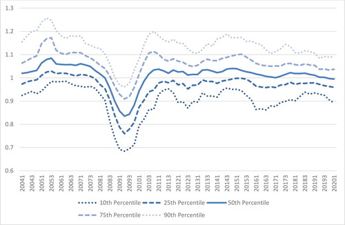We use a two-quarter lag between the sale price and the adjusted estimated value to ensure that the appraisal is independent from the subsequent sale. Whereas more than 150 sales occurred during some quarters, there were only 16 sales across all property types during 2009Q1. To smooth out some of the quarterly variations, we consider sales over three quarters (the previous, current, and next quarters) as shown in Figure 1. The number of sales is broken down by type of market. Figure 2 depicts the medians and selected quantiles for the ratios of sale prices to appraised values averaged over three quarters.⁴ Focusing on the median ratios, appraised values appear to be 5% below transaction prices prior to the GFC, while properties transacted some 15% below their estimated value at the height of the GFC. After the GFC, prices again slightly exceeded appraised values. This is consistent with the much documented smoothing and lagging of appraisals and the effects of these throughout the cycle.

Figure 1. Cumulative number of sales. Note: The figure displays the three-quarter (centered) cumulative number of true sales in the cleaned dataset.

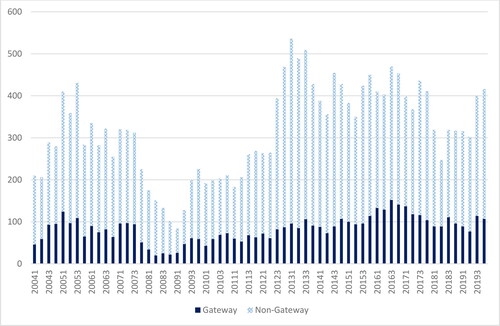
Figure 2. Ratios of sale prices to appraised values. Note: The figure depicts the median (50th percentile) of the three-quarter average of the ratio of sale price to the lagged appraised value as well as the 10th, 25th, 75th, and 90th percentiles.

We use the empirical distribution of ratios at time $q$ to determine the expected sale price of unsold properties at time $q$ rather than $q+1$ as in the production of the NCREIF transaction-based index (NTBI). This is to take into account the well-documented escrow lag in commercial real estate; transaction prices were agreed upon several weeks prior to their recording. The one quarter lag we use is consistent with the 90-day escrow lag that is discussed in Hoesli et al. (2015). Given the selected quantile order ($Q_o$), the expected sale price of unsold properties is calculated as: (2) $${\mathit{ESP}}_{p,q}={\mathit{AEV}}_{p,q-1}·Q_o\left({\mathit{SPAEV}}_q\right)$$(2) where ${\mathit{ESP}}_{p,q}$ is the expected sale price of property $p$ at time $q,$ ${\mathit{AEV}}_{p,q-1}$ is the adjusted estimated value of property $p$ at time $q-1,$ and $Q_o\left({\mathit{SPAEV}}_q\right)$ is the empirical quantile of order $o$ of the ratio of sale prices to adjusted estimated values for quarter $q.$

Method

In this section, we first focus on the classification between gateway and non-gateway markets. We then discuss how we construct the simulated portfolios, before presenting the performance metrics that are computed for our simulated portfolios. We continue with a discussion of the property quality controls that we implement as part of the robustness checks. Finally, we present the methods we use for our mixed-asset portfolio and systematic risk analyses, respectively.

Gateway Versus Non-Gateway Markets

It is generally understood that gateway cities are large cities, with large international airports, economies that are globally connected, and status. Historically, they have developed as ports of entry into a country. Conventional wisdom and prior research (Devaney et al., 2019; Feng et al., 2022; Ling et al., 2019) consider Boston, Chicago, New York, Los Angeles, San Francisco, and Washington, D.C. as gateway markets. We use this six-city definition as our initial set of gateway markets. Looking at GDP figures at the MSA level, those cities rank in the top four (New York, Los Angeles, Chicago, and Washington, D.C.), sixth (San Francisco), and seventh (Boston) in the country.

An important consideration is whether the whole MSAs should be considered as gateway or only some divisions. For the six markets and for each property type (apartment, industrial, office, and retail), we analyzed capitalization rates and percent leased for the main division and then assessed whether the other divisions within the same MSA exhibited similar values for those metrics or not. Divisions with a similar level and pattern over time for those metrics as the main division are also considered to be gateway. With the exception of Los Angeles, there are clear differences within MSAs, indicating that only parts of those are to be considered gateway markets. Appendix 1, Panel A shows our classification of divisions for the six gateway markets.

For robustness check purposes, we consider four other definitions of gateway markets: two expanded and two restricted sets. The two expanded sets are defined using 2003 GDP figures at the MSA level from the Bureau of Economic Analysis.⁵ The first set considers markets that account for at least 2.4% of national GDP. This results in Dallas and Philadelphia being added to the initial six gateway markets. The second set uses a threshold of 2.2%. This leads to Atlanta, Houston, and Miami being also considered to be gateway markets. Appendix 1, Panel B shows the classification of divisions for those additional markets. We also consider two restricted sets of markets. The first one only includes the three largest markets (New York, Los Angeles, and Chicago), while the second set additionally considers the fourth largest market (Washington, D.C.).

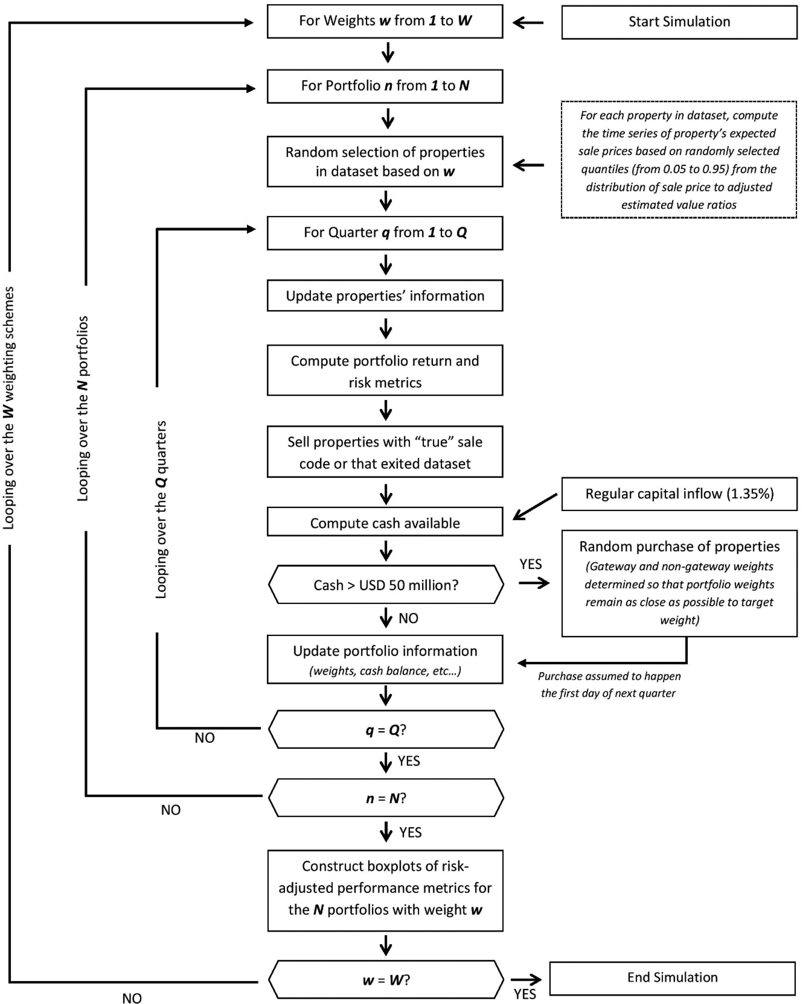
Portfolio Simulations

Appendix 2 presents the flowchart of our simulation process. For a given amount of assets under management (AUM), we use Monte Carlo simulations to construct hypothetical portfolios with various weights of gateway and non-gateway markets. We start with gateway markets only, and modify weights by 10% increments until reaching portfolios with non-gateway markets only.⁶ For each set of weights, we construct 1,000 hypothetical portfolios. Given the stringent filtering rules used to clean up the database, the population from which the portfolios are drawn is representative of the institutional investment universe and hence we do not apply any stratification to the sampling scheme above that concerning location. Hence, we construct N (= 1,000) portfolios of P properties (varies depending on the AUM assumption) for each of the W (= 11) weighting schemes. Using a fully random selection approach for properties, instead of actual portfolios, permits removal of any asset picking advantage that a manager may have. Finally, note that a specific property can be included in multiple portfolios but only once in a given portfolio.

A crucial parameter in the simulation analyses is AUM. We start by considering an amount of USD 5 billion to be invested as of the beginning of 2004. We also use an amount of 2.5 and 7.5 billion, respectively, to assess whether portfolio size impacts upon the results. The amount invested is incremented to reflect the growth in assets managed by institutional investors over time. To proxy for such growth, we use data concerning U.S. total retirement assets as published by the Investment Company Institute.⁷ We then estimate the value of real estate holdings by applying the allocations to real estate by all plan sponsors as published in various Pension Real Estate Association (PREA) reports and remove the effect of commercial real estate capital returns as measured by NCREIF index returns. We obtain an average annual growth in real estate holdings from 2004 to 2019 of 5.5%; hence, we apply a quarterly rate of increase of 1.35% to the invested capital at the beginning of each quarter. This results in a compound increase in invested capital that is independent from portfolio performance. We use a constant rather than time-varying rate to insure that our results are not affected by market timing. The increases in invested capital lead to additional properties being incorporated in our portfolios. This is desirable given the significant increase in the number of properties in the NCREIF database.

In addition to the growth in invested capital over time, we also take into account properties that exit the dataset without there being a true sale.⁸ These properties are removed from portfolios as of the quarter prior to their exiting the dataset at their expected sale price. As explained in “Property Value Adjustments,” the expected sale price of property $p$ at time $q$ is calculated by multiplying the adjusted estimated value at time $q-1$ by the empirical quantile of order $o$ of the ratio of sale prices to adjusted estimated values for quarter$q.$ At each portfolio inception, we draw for each property the order $o$ that will be used to sample empirical quantiles for the entire lifespan of the property. For example, if the selected order for a given property is 0.5 (i.e., the median), then we use the median of the ratios of sale price to adjusted estimated value computed for each quarter. So, for this example, we compute the expected sale price for quarter$q$ on the basis of the median of the ratios pertaining to that period. Note that the order of the quantile is drawn randomly without taking into account the characteristics of properties. As such, the quantile for a given property will change with each iteration. Using quantiles rather than a measure of central tendency is useful to generate heterogeneity in simulation results, making it possible to explore more widely the solution space.

In the case of true sales, properties exit our portfolios at the reported sale price. For those properties, we know the true ratio of sale price to adjusted market value. We can thus determine the quantile order of the ratio within the distribution of ratios for that quarter. We use this quantile order to calculate the expected sale price of that property for previous quarters.

The proceeds from the sale and exiting of properties are combined with the increase in investment capital as well as the other items affecting cash flows and added to the initial cash balance to determine the funds available for purchases for a given quarter: (3) $${\mathit{FAP}}_{n,q}={CB}_{n,q-1}+{\Delta IC}_q+{\mathit{PSE}}_{n,q}+{\mathit{OCF}}_{n,q}$$(3) where ${\mathit{FAP}}_{n,q}$ are the funds available for purchases for portfolio $n$ during quarter $q,$ ${CB}_{n,q-1}$ is the cash balance at the beginning of quarter $q,$ ${\Delta IC}_q$ is the change in invested capital during quarter $q,$ ${\mathit{PSE}}_{n,q}$ are the proceeds from the sale and exiting of properties during quarter $q,$ and ${\mathit{OCF}}_{n,q}$ are the other items affecting cash flows during quarter $q.$ The other items affecting cash flows include NOIs, capital expenditures, and partial sales. Provided that the funds available exceed USD 50 million, they are used to purchase additional properties, maintaining portfolio weights for gateway and non-gateway markets as close as possible to targets.

At the end of the simulations, we check for the amount of cash held in portfolios as well as for the weights of gateway and non-gateway markets. Specifically, we remove any portfolio containing more than 2% of AUM in cash in absolute value or whose gateway weight deviates by more than 500 basis points in absolute value from its target allocation.

Performance Metrics

Various portfolio performance metrics are calculated for the 11 sets of 1,000 portfolios, and we compare metric distributions across the 11 sets. We first calculate annualized total, income, and appreciation returns for each simulated portfolio. Returns are calculated using the NCREIF methodology, replacing their market values by our expected sale prices. We also consider portfolio standard deviations, which provide for an analysis of variations through time. We further calculate the Sharpe ratios, value-at-risk (VaR), and maximum drawdown (MDD). For the Sharpe ratios, we use the three-month Treasury rate sourced from the Federal Reserve Bank of St. Louis. ${\mathit{VaR}}_{\alpha }$ is calculated as the return level for which we expect a proportion $1-\alpha$ of the returns to be below that threshold. So, computing ${\mathit{VaR}}_{\alpha }$ involves solving the following equation for a given level of $\alpha$: (4) $$P\mathrm{ }\left[\mathit{Return}<{\mathit{VaR}}_{\alpha }\right]=1-\alpha$$(4) where we define $\mathit{Return}$ as the trailing appreciation return compounded over four quarters. We consider both 95% and 99% confidence levels. MDD is the maximum capital loss from a peak to a trough over the simulation period: (5) $$\mathit{MDD}=\underset{t\in (0,T)}{\max }\left\{-\frac{\left(C_t-\mathrm{ }{\mathit{RunMax}}_t\right)}{{\mathit{RunMax}}_t}\right\}$$(5) where ${\mathit{RunMax}}_t\mathrm{ }$ is the highest peak (i.e., running maximum) observed during the period going from $0$ to $t$ and $C_t$ is the capital value at time $t.$ Examples of the limited use of those downside risk measures for direct real estate investments include Gordon and Tse (2003), Hamelink and Hoesli (2004), and Amédée-Manesme et al. (2015). We also calculate the recovery time, that is, the number of years needed for the capital value to regain its pre-drawdown level from the trough.

Portfolio Analyses

As a further means of investigating the usefulness of diversifying across gateway and non-gateway markets, we construct efficient frontiers with stocks, bonds, and gateway and non-gateway real estate in an unlevered setting. For stocks, we use the MSCI USA total return index, while the Bloomberg Barclays U.S. Government 10-year total return index is used for bonds. The analysis is first undertaken using median total returns from our simulations for the two types of real estate markets. For gateway markets, access to market information is likely to be homogeneous for domestic and international investors (Devaney et al., 2019) and hence we maintain that all investors will achieve a return akin to that of the simulation median returns. For non-gateway markets, however, information asymmetry is likely to occur, with local players at an advantage. To reflect varying information levels for non-gateway markets, we also perform portfolio analyses using the returns for the 0.65 and 0.35 percentiles, respectively, for non-gateway markets. The 0.65 (0.35) percentile highlights the performance of an investor having an information advantage (disadvantage) on non-gateway markets. The underlying intuition is that an investor with an information advantage will be able to select properties in such a way that portfolio performance will exceed the median. The reverse reasoning applies to an information disadvantage.

Quality Controls

The numerous filtering rules applied during the data cleaning process were intended to keep only properties deemed of investment-grade quality. We notably discarded properties with sale codes, NOIs, or capital expenditures that were considered to be too extreme. Additional controls for property quality are considered as robustness checks. As the NCREIF database does not contain variables pertaining to property quality, we have developed three metrics that can serve as a proxy for property quality.⁹

The first two quality metrics use a normalized ratio of NOI per square foot, calculated for each property $p$ in every quarter $q.$ The underlying idea of those metrics is that the level of a property’s NOI relative to that of comparable properties is a valid proxy for the quality of this property. For each metric, we compute the following ratio: (6) $${\mathit{QualityMetric}}_{p,q}=\frac{{\mathit{NOI}\_\mathit{SqFt}}_{p,q}\mathrm{ }-\mathrm{ }\mathit{Avg}\left({\mathit{NOI}\_\mathit{SqFt}}_{\mathit{comp},q}\right)}{\mathit{StDev}\left({\mathit{NOI}\_\mathit{SqFt}}_{\mathit{comp},q}\right)}$$(6) where ${\mathit{QualityMetric}}_{p,q}$ is the quality metric for property $p$ in quarter $q,$ ${\mathit{NOI}\_\mathit{SqFt}}_{p,q}$ and ${\mathit{NOI}\_\mathit{SqFt}}_{\mathit{comp},q}$ are the NOIs per square foot in quarter $q$ for property $p$ and for comparable properties, respectively. The difference between the first and second proxy for quality lies in the definition of comparables. In the first approach, the comparable properties are all properties located in the same CBSA (or division for gateway markets) and of the same property type as property $p.$ When there are fewer than five comparable properties, we use all properties of the same type located in CBSAs with not enough comparables (i.e., fewer than five comparables). In the second approach, we normalize the NOIs per square foot using all properties of the same type in the same division for gateway properties and all properties of the same sector in the same market class (i.e., secondary or tertiary) for non-gateway properties.¹⁰ For both approaches, we discard properties for which the absolute value of ${\mathit{QualityMetric}}_{p,q}$ is greater than one for more than 10% of the quarters. The underlying objective is to retain only properties of homogenous quality. We end up with cleaned datasets of 5,546 and 6,621 properties, respectively.

The third approach uses the property’s age as a proxy for property quality. As the age variable contained in the NCREIF database is only a crude proxy for quality given that it is not corrected to take into account refurbishments, we construct a new variable where the age of each property is adjusted to account for the amounts spent in capital expenditures. First, for each property $p$ and at each quarter $q,$ we compute a renovation cost threshold, as follows: (7) $${\mathit{RCT}}_{p,q}=\mathrm{ }{\mathit{SqFt}}_{p,q}·{RC}_{c,q}$$(7) where ${\mathit{RCT}}_{p,q}$ and ${\mathit{SqFt}}_{p,q}$ are the renovation cost threshold and the number of square feet of property $p$ in quarter $q,$ respectively, and ${RC}_{c,q}$ is the renovation cost per square foot for CBSA $c$ in quarter $q.$ ${RC}_{c,q}$ is computed using a hypothetical renovation cost of USD 100 per square foot as of Q4 2019 and adjusted over time and across markets using construction cost information from RSMeans (2018).¹¹ We then compute the cumulative 12-quarter trailing capital expenditures, ${\mathit{TTQ}\_\mathit{CapEx}}_{p,q},$ as: (8) $${\mathit{TTQ}\_\mathit{CapEx}}_{p,q}=\sum _{i=0}^{11}{\mathit{CapEx}}_{p,q-i}+\min (0,\mathrm{ }\sum _{i=1}^4{\mathit{CapEx}}_{p,q+i})$$(8) where ${\mathit{CapEx}}_{p,q}$ are the capital expenditures for property $p$ in quarter $q.$ The minimum function is used to control for capital expenditures that have been overturned (recorded as negative values in the database) in the year following their booking. To correct the age of a property $p,$ we consider that, if ${\mathit{TTQ}\_\mathit{CapEx}}_{p,q}$ exceeds the renovation cost threshold ${\mathit{RCT}}_{p,q}$ in a given quarter $q,$ the property is considered to be fully renovated and its age is set to zero in quarter $q.$ Note that any subsequent renovation is not considered until at least 3 years after the current renovation. A property remains in the database as long as its adjusted age is less than or equal to 20 years (and it has at least four quarters of data). This results in 5,352 properties being in the database.

Systematic Risk

We consider systematic risk across types of markets by estimating, for each weighting scheme, the following regression: (9) $${TR}_n-r_f\mathrm{ }={\beta }_0+{\beta }_1·(\mathit{Mkt}-r_f)+{\epsilon }_n$$(9) where ${TR}_n$ is the vector of quarterly total returns for portfolio $n,$ $r_f$ is the vector of risk free rates over the same period, and $\mathit{Mkt}$ is the vector of market returns. The market is a capitalization-weighted composite index of U.S. stocks, government bonds, corporate debt, securitized debt, and real estate. The real estate weight is approximated using a fixed percentage (42.9%) between the value of real estate and GDP. The percentage is calculated based on the figures contained in various issues of the Total Markets Table as published by the European Public Real Estate Association (EPRA). We use the following indexes to proxy for asset class returns: MSCI USA Index, Bloomberg Barclays U.S. Treasury Index, Bloomberg Barclays U.S. Securitized: MBS/ABS/CMBS and Covered Index, and Bloomberg Barclays U.S. Corporate Bond Index. Real estate returns are computed from our sample of properties using the median ratio of the sale price to adjusted estimated value to account for appraisal smoothing. We also performed the regressions using an index both as the dependent variable and as the real estate component in the composite index. The indexes include the NPI, the NTBI, and an index constructed using our method to adjust for appraisal smoothing. The models are estimated using OLS.

Results

We first present descriptive statistics and graphs for our simulated portfolios. The performance analyses for portfolios containing varying weights of gateway and non-gateway markets are discussed next. The following section contains various robustness checks, while the second to last section provides our portfolios analyses. A final section provides a discussion of systematic risk.

Simulated Portfolios

With respect to the number of properties in simulated portfolios, the median number of properties in the full portfolios as of the beginning of the time period ranges from 83 (when the portfolio is entirely invested in gateway properties) to 151 (when the entire allocation is in non-gateway markets). Some sub-portfolios contain only a limited number of properties when the weight of the related market type is small. For instance, if 10% of a portfolio is allocated to gateway markets, the median number of gateway properties is only 11 and the minimum is 1. However, in most instances, portfolios contain a sufficient number of properties to achieve proper diversification. At the end of the time period, the median number of properties in portfolios is markedly larger (in the 215–369 range), reflecting the growth of AUM over time, and the minimum number of properties in sub-portfolios is never below 16.

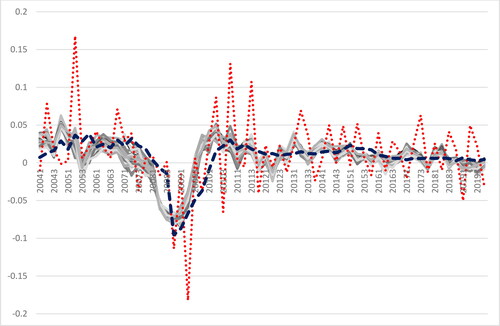
Figure 3 shows appreciation returns for 30 portfolios with varying weights for gateway markets, as well as returns for the NPI and the NTBI. The figure shows return patterns that are consistent with the well-documented cyclical nature of commercial real estate markets. Our portfolio returns are more volatile than NPI returns. This is to be expected given that the NPI is appraisal based, whereas the values of the properties in our portfolios are adjusted. On the other hand, as we implemented a method to filter out the noise resulting from the highly variable number of sales over time, our portfolio returns are less volatile than those of the NTBI.

Figure 3. Portfolio and market appreciation returns. Note: The solid lines are the returns of 30 randomly selected portfolios, the dashed line is the NCREIF Property Index (NPI), and the dotted line the value-weighted NCREIF Transaction-Based Index (NTBI).

Performance Analysis

Figure 4 depicts the distributions of portfolio annualized total returns, standard deviations, and Sharpe ratios for the base case analysis and for robustness checks pertaining to property quality (discussed in the next section). Each boxplot shows the median (thick line) and the 25% and 75% percentiles (the edges of the box). The whiskers represent the most extreme data points or one and a half the interquartile range, depending on which one is the least extreme. Any observation lying outside of the whiskers can be considered an outlier. Panel A shows that the median portfolio total return diminishes monotonously as a larger weight is allocated to non-gateway markets (median return of 8.40% for gateway markets versus 7.65% for non-gateway markets). Panel A also shows that the distribution of gateway total returns is almost symmetrical (skewness of 0.05). On the other hand, as we move to a larger weight for non-gateway markets, distributions exhibit positive asymmetry (skewness for non-gateway markets of 0.63).

Figure 4. Distributions of portfolio total returns, standard deviations, and Sharpe ratios. Note: BC = base case, NR = quality control using NOI ratios, NRM = quality control using NOI ratios by market class, and AC = age-corrected quality control. 1.0, 0.5, and 0.0 indicate the allocation to gateway markets (100%, 50%, and 0%, respectively).

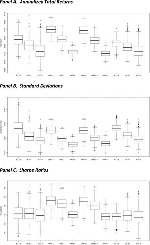
In line with median returns, the standard deviations (Panel B) also diminish as a larger fraction of a portfolio is allocated to non-gateway markets (median standard deviation of 5.33% and 4.92% for gateway and non-gateway markets, respectively). Also, the dispersion of portfolio standard deviations diminishes as the weight of non-gateway markets increases. As a result, the portfolio Sharpe ratios do not vary depending on the share of gateway and non-gateway markets (Panel C). It is interesting to contrast our results with those of Beracha et al. (2017), who find that high capitalization rate properties dominate low capitalization rate properties on a risk-adjusted basis for the period 1978–2015. Our results suggest that there is no difference in performance across non-gateway and gateway markets, although the former have higher capitalization rates than the latter, with the exception of a few quarters at the beginning of the time period. Those diverging results are likely due to differences in time periods and data filtering rules (our filtering rules do not accommodate for value-added properties).

We now turn to analyzing the two components of total returns. Figure 5, Panel A, shows that median income returns are 50 basis points larger for non-gateway markets (5.77%) than for gateway markets (5.27%). Income returns exhibit a slight negative asymmetry (skewness from −0.12 to −0.32), with no clear trend with respect to the market type weight. Negative asymmetry would be expected for income returns as NOI surprises are more likely to be on the downside than the upside. Income returns for non-gateway markets are also less volatile than their gateway counterparts.

Figure 5. Distributions of annualized portfolio income and appreciation returns. Note: BC = base case, NR = quality control using NOI ratios, NRM = quality control using NOI ratios by market class, and AC = age-corrected quality control. 1.0, 0.5, and 0.0 indicate the allocation to gateway markets (100%, 50%, and 0%, respectively).

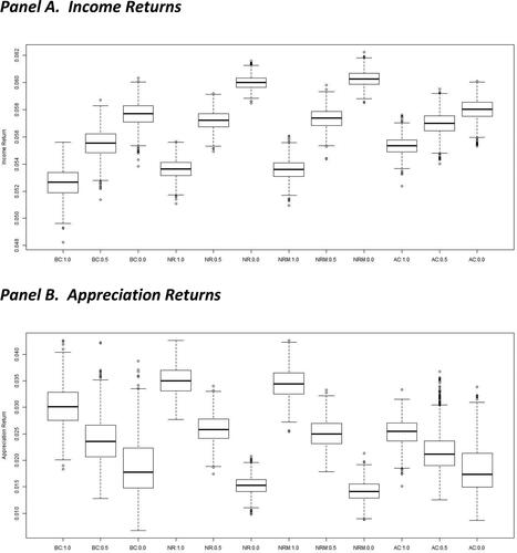
Given that the NOI does not provide the full picture regarding the cash flow generating ability of assets, we calculated the free cash flow return as the NOI minus capital expenditures divided by the property’s market value at the beginning of the period. Free cash flow returns are approximately 150 basis points lower than income returns, with capital expenditures only 12 basis points higher for non-gateway markets. Hence, non-gateway markets offer significantly higher recurrent returns than gateway markets even after accounting for capital expenditures. These results should be of interest to institutional investors looking for sizeable and recurrent cash flows to meet their commitments.

Focusing on the appreciation return component, Figure 5, Panel B, shows that gateway markets have a 123 basis point larger median return (3.01%) than their non-gateway counterparts (1.78%). This result is consistent with the greater productivity of larger cities as discussed in the urban economics literature. Higher economic growth in gateway markets translates into greater remuneration increases for the production factors, which directly and indirectly lead to faster appreciation in commercial real estate values. Over the period, non-gateway markets on average did not provide capital protection in real terms, given that the average compound inflation rate during the 2004–2019 period was 2.08%. A minimum allocation of 30% in gateway markets would have been warranted to insure preservation of the invested capital in real terms. Gateway capital returns also come with a somewhat larger dispersion than is the case for non-gateway markets.

Figure 6, Panel A, indicates that the 95% VaR is somewhat greater for gateway markets (19.6%) than for non-gateway markets (18.0%).¹² The MDD results (Panel B) further suggest that downside risk is greater for gateway markets (31.5%) than for non-gateway markets (30.4%). Unsurprisingly, these drawdowns occurred during the GFC. From a practical perspective, this analysis does not indicate material differences in downside risk across gateway and non-gateway markets. This seems consistent with the conclusion that capital market integration (i.e., co-movements in capitalization rates) is greater than space market integration (i.e., co-movements in NOIs), as discussed in Van Dijk and Francke (2021).

Figure 6. Portfolio downside risk measures. Note: BC = base case, NR = quality control using NOI ratios, NRM = quality control using NOI ratios by market class, and AC = age-corrected quality control. 1.0, 0.5, and 0.0 indicate the allocation to gateway markets (100%, 50%, and 0%, respectively).

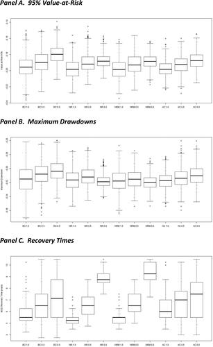
For investors, capital loss measures, albeit important, are not sufficient in ascertaining the riskiness of portfolios. A complementary metric is the recovery time, i.e., the number of years needed to revert to the pre-drawdown portfolio high-water mark. As a consequence of differences in appreciation returns across markets, Figure 6, Panel C, shows that the median recovery length is shorter for gateway markets (5.5 years) than for non-gateway markets (7.1 years). The dispersion of recovery times is lower for gateway portfolios, which reinforces the idea that those markets are quicker to recover. Nonetheless, portfolios that are heavily tilted toward gateway markets exhibit stronger positive skew than their non-gateway counterparts as evidenced by the outliers. As asset values will take longer to regain the level of the associated liabilities, non-gateway portfolios are at a disadvantage in an asset-liability management (ALM) framework. This is even more of an issue for leveraged investors, especially if the lender is monitoring closely the loan-to-value (LTV) ratio as part of the agreed covenants.

Robustness Checks

The first set of robustness checks pertains to the market definition, the second to property quality, and the third to sectors.¹³

With respect to the first set of robustness checks, we consider four sets of gateway markets in addition to the base case definition. The sets range from a 3-market definition to an 11-market definition. For each set of markets, we report in Table 2 various performance metrics for three types of portfolios (gateway weight of 100%, 50%, and 0%). For each metric, the table also shows the difference in performance between 100% gateway and 100% non-gateway portfolios. Overall, the performance spreads have the same sign and are of similar magnitude, suggesting that our results are robust to the definition being used.¹⁴ Widening the definition of gateway markets from our base case leads to more muted differences between gateway and non-gateway markets. Narrowing the definition of markets from the original set shows that the four-market set provides slightly less discrimination across markets, while the three-market definition is comparable with the base case. We conclude that the original set of six gateway markets is appropriate, corroborating the conventional wisdom.¹⁵ A set of six markets has the further advantage of widening the universe of investment opportunities as compared with the second best solution with three markets.

Table 2. Selected Performance Metrics for Various Sets of Gateway Markets.

	Total Returns (%)				Income Returns (%)
Gateway Weight	1.0	0.5	0.0	Δ	1.0	0.5	0.0	Δ
3 Markets	8.4	8.1	7.8	65	5.2	5.5	5.7	−48
4 Markets	8.2	8.1	7.9	29	5.3	5.5	5.7	−44
6 Markets (Base Case)	8.4	8.0	7.6	75	5.3	5.6	5.8	−50
8 Markets	8.2	8.0	7.8	49	5.3	5.6	5.8	−46
11 Markets	8.1	7.9	7.7	41	5.4	5.6	5.8	−40
	Standard Deviation of Total Returns (%)				Standard Deviation of Income Returns (%)
Gateway Weight	1.0	0.5	0.0	Δ	1.0	0.5	0.0	Δ
3 Markets	5.4	5.1	5.0	48	0.4	0.4	0.4	3
4 Markets	5.4	5.1	5.0	40	0.4	0.4	0.4	3
6 Markets (Base Case)	5.3	5.1	4.9	41	0.4	0.4	0.3	7
8 Markets	5.2	5.0	4.9	29	0.4	0.4	0.3	5
11 Markets	5.2	5.0	4.9	24	0.4	0.3	0.3	3
	Maximum Drawdown (%)				95% VaR (%)
Gateway Weight	1.0	0.5	0.0	Δ	1.0	0.5	0.0	Δ
3 Markets	−31.9	−31.0	−30.3	−167	−19.8	−19.3	−18.4	−138
4 Markets	−30.4	−30.6	−30.8	37	−18.8	−18.8	−18.8	−6
6 Markets (Base Case)	−31.5	−30.8	−30.4	−111	−19.6	−19.0	−18.0	−159
8 Markets	−31.1	−30.7	−30.4	−71	−19.3	−18.8	−18.2	−114
11 Markets	−30.7	−30.7	−30.4	−28	−19.1	−18.8	−18.3	−80

Notes: Δ denotes the spread in basis points between 100% gateway and 100% non-gateway markets. 3 Markets = New York, Los Angeles, and Chicago; 4 Markets = New York, Los Angeles, Chicago, and Washington D.C.; 6 Markets = New York, Los Angeles, Chicago, Washington D.C., Boston, and San Francisco; 8 Markets = New York, Los Angeles, Chicago, Washington D.C., Boston, San Francisco, Dallas, and Philadelphia; and 11 Markets = New York, Los Angeles, Chicago, Washington D.C., Boston, San Francisco, Dallas, Philadelphia, Atlanta, Houston, and Miami.

In addition to the results for the base case analysis, Figures 4–6 also report the results for the robustness checks that we undertake to control for the quality of properties.¹⁶ Overall, these results provide strong support to our previous conclusions, both regarding returns and downside risk.¹⁷ If anything, the spread in returns between gateway and non-gateway markets tends to be more pronounced when property quality is accounted for. However, two differences are worth mentioning. First, as the difference in total returns between types of markets is wider after controlling for quality, with standard deviations by and large constant relative to the base case analysis, the Sharpe ratios are slightly in favor of gateway markets (Figure 4, Panel C). Second, for non-gateway portfolios, controlling for property quality has the effect of trimming the lower part of the recovery time distributions, possibly because high quality properties are excluded from the analysis (Figure 6, Panel C). Hence, recovery times are longer (the median increases roughly from seven to nine years) and more homogenous for non-gateway markets.

The discussion of performance metrics in “Performance Analysis” refers to portfolios that can include assets of any sector. We now take sectors into account, which is useful for at least two reasons. First, considering all sectors simultaneously may reveal differences in performance that are attributed to the type of markets (gateway versus non-gateway), whereas they can be explained by different sector weights. Second, some investors may favor a given sector over others, for example, if they have developed an expertise that is specific to a sector. The analyses are undertaken for an AUM of USD 2.5 billion to account for the smaller pool of properties available at the sector level.

We consider first a sectoral composition for both gateway and non-gateway markets that is equal to the sectoral composition of the entire sample (rather than that by type of market) at the beginning of each quarter. By doing so, any differences in performance will be due purely to the type of market. This results mainly in a lower weight for office properties and a higher allocation for retail in gateway markets, while the changes in allocations are in the opposite direction for non-gateway markets. The results in Figure 7 show that our conclusions pertaining to the performance of gateway and non-gateway markets are not driven by differences in sectoral composition across market types.

Figure 7. Robustness checks for sectoral composition and sectors. Note: BC = base case, CSW = constant sector weights, APT = apartments, IND = industrial, OFF = office, and RET = retail. 1.0, 0.5, and 0.0 indicate the allocation to gateway markets (100%, 50%, and 0%, respectively).

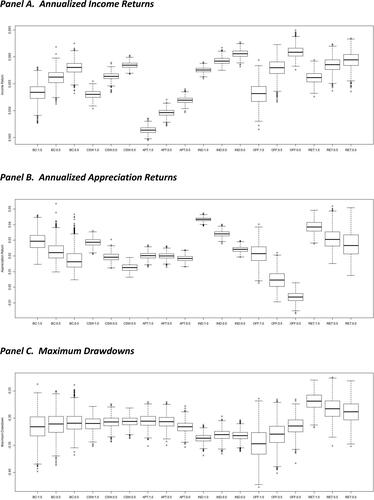
Results in Figure 7, Panel A, further suggest that the difference in income returns between non-gateway and gateway markets is of similar magnitude across all sectors. However, Panel B points to noteworthy differences across sectors with regard to appreciation returns. Whereas the appreciation return spread between gateway and non-gateway markets is 129 basis points in the overall analysis, the spread is markedly higher for office and industrial properties (281 and 191 basis points, respectively). For retail, the spread (118 basis points) is in line with the overall spread, whereas, for apartments, it is much lower (18 basis points). The wider spreads for office and industrial properties than for retail and residential assets is consistent with economic intuition. In contrast to office and industrial properties, which are important production factors, the residential sector is not a production factor per se. As such, it will capture productivity gains only indirectly and partially through increases in wages, which could explain the lower spread in appreciation returns across market types. Despite being production factors, retail properties are also largely dependent on household spending, notably due to sales-based rents. Accordingly, the spread for that sector is lower than for office and industrial properties but higher than for apartments. Finally, Panel C shows that the main conclusion pertaining to downsize risk, that is, that gateway markets tend to be slightly riskier than non-gateway markets holds across sectors, with the exception of apartments, which tend to be slightly riskier in non-gateway markets.

Portfolio Analyses

Figure 8, Panel A depicts the composition of portfolios containing stocks, bonds, and both gateway and non-gateway markets in an unlevered setting.¹⁸ Median returns from our simulations are used for the two types of real estate markets. The allocation to real estate in mixed-asset portfolios is large, with non-gateway markets appearing in low-risk portfolios while gateway markets constitute the preferred investment route for medium- to high-risk portfolios.

Figure 8. Composition of mixed-asset portfolios.

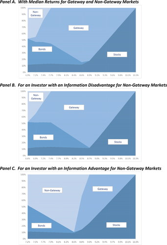
To analyze the effects of information asymmetry on non-gateway markets, we consider both an information disadvantage (Panel B) and an information advantage (Panel C). An information disadvantage does not lead to any differences in portfolio allocations. Non-gateway markets are still useful in low-risk portfolios and this remains true even for high information disadvantages (i.e., the 0.05 percentile). Non-local investors, who are more likely to be at a disadvantage on such markets, should still consider non-gateway markets. On the other hand, an information advantage leads to a substitution of gateway markets by non-gateway markets up to the middle of the frontier. Hence, an investor with even a slight information advantage should increase markedly the allocation to non-gateway markets. This result is reinforced as one moves to higher percentiles and, for top-tier performers (i.e., percentiles equal or over 0.7), the allocation should be entirely to non-gateway markets.

Analysis of Systematic Risk

This section contains a discussion of regression results for Equation (9)(9) $${TR}_n-r_f\mathrm{ }={\beta }_0+{\beta }_1·(\mathit{Mkt}-r_f)+{\epsilon }_n$$(9) . Figure 9 depicts the distributions of regression adjusted R-squared (Panel A) and of estimated coefficients for systematic risk over the whole sample period (Panel B) for 11 weighting schemes. It also shows (Panel C), for three weighting schemes, the estimated coefficients for systematic risk for two time periods (2004Q1–2011Q4 and 2012Q1–2019Q4). The adjusted R-squared amount to approximately 0.15 and increase slightly with the weight allocated to non-gateway markets. Systematic risk appears to be the same across market types and its median value across samples is 0.47, with all coefficients significant at the 5% level. Panel B also shows that systematic risk is quite narrowly distributed with coefficients ranging from approximately 0.32 to 0.56, with slightly less dispersion across non-gateway portfolios. We also performed the regressions at the index level and obtained median beta coefficients of 0.29 (NPI), 0.34 (NTBI), and 0.45 (our desmoothing method), respectively. Those results are consistent with the well-known smoothing bias of the NPI and the potential issues of the NTBI, which lead to lower measures of systematic risk. We additionally classified portfolios based on their total return, rather than by market type, and again found no differences between groups.

Figure 9. Distributions of adjusted R-squared and portfolio betas. Note: T1 = 2004Q1–2011Q4 and T2 = 2012Q1–2019Q4.

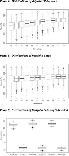
Although systematic risk is constant across markets, it exhibits much variability over time (Panel C). As would be expected, during the first subperiod (which includes the GFC), median betas are much higher (0.72) than during the second subperiod (0.05), highlighting the fact that during a crisis asset returns tend to be much more correlated. Again, there are no material differences across types of markets.

Conclusions

Using simulation analysis and property-level data, we compare various return and risk metrics for portfolios with varying exposures to gateway and non-gateway markets. The sample distributions of performance metrics provide an accurate depiction of the return and risk of the different types of real estate markets. We also analyze how best to diversify a mixed-asset portfolio across gateway and non-gateway markets. All analyses are conducted using property values that have been corrected using an innovative procedure to reflect market values more accurately.

Our results show that gateway markets have a higher total return and standard deviation than their non-gateway counterparts, leading to comparable risk-adjusted performance across types of markets. Differences in standard deviations are not attributable to differences in systematic risk given that the latter is comparable across market types. Non-gateway markets have a significantly higher income return than gateway markets, even after accounting for capital expenditures. On the other hand, and consistent with economic intuition, gateway markets exhibit higher appreciation returns. Gateway markets appear to have slightly higher downside risk than their non-gateway counterparts; however, recovery times are shorter for the former than for the latter, consistent with the higher appreciation returns for gateway markets. Non-gateway markets are useful in diversifying low-risk mixed-asset portfolios, while gateway markets should constitute the entire allocation for riskier portfolios. An information disadvantage on non-gateway markets does not alter this conclusion, but an information advantage leads to a substitution of gateway markets by their non-gateway counterparts.

Changing the set of gateway markets does not alter our main findings, although a six-market definition has most appeal, corroborating a common practice of institutional investors. Our results are also shown to be robust when sectoral weights are held constant across the two types of markets, when property quality is controlled for and when alternative AUM assumptions are considered. Income returns are consistently larger for non-gateway markets than for gateway markets across all sectors. On the other hand, total and appreciation returns are larger for gateway than for non-gateway markets in all sectors, except apartments.

There are various ways in which our knowledge of real estate gateway markets could be expanded. First, it would be interesting to analyze how the importance of a metropolitan area can change over time. Obvious examples of metropolitan areas that have grown fast during the period are San Francisco, Dallas, or Houston. Second, considering property subtype heterogeneity seems warranted. For instance, rather than referring to the broad category of retail properties, one could consider shopping malls versus high-street retail. Third, a more granular set of areas than metropolitan divisions could be used to delineate markets in order to capture the effects of micro-location more precisely. Finally, a fruitful avenue for future research would be to analyze whether our main conclusions hold for other regions or globally. There are many international gateway markets, such as Toronto, Paris, London, or Tokyo, and comparing commercial real estate performance between those cities and more regional markets should prove informative.

Acknowledgments

We are grateful to the Real Estate Research Institute (RERI) for having supported this project financially. Our RERI mentors, Martha Peyton and Greg MacKinnon, seminar participants at the Royal Institute of Technology in Stockholm (Sweden), the University of Neuchâtel (Switzerland), and the European Commercial Real Estate Data Alliance (E-CREDA) annual conference provided many useful comments and suggestions. Two anonymous reviewers provided very constructive remarks that have much improved the quality of the article. We also thank NCREIF for providing us with the data. Jeff Fisher was very helpful in helping us secure those data and provided many valuable inputs regarding the data as well as the method that NCREIF used until recently to produce its TBI. The usual disclaimer applies.

Additional information

Funding

This article was supported financially by the Real Estate Research Institute.

Notes

1 We only consider sales that are classified by NCREIF as being true sales.

2 Due to the lack of transactions in 2020, the NCREIF transaction-based indexes have been discontinued.

3 In the latter case, the value is that of the previous quarter adjusted for any capital expenditures or partial sales.

4 We also calculated the ratios of sale price to the lagged appraised value for gateway and non-gateway markets separately. Given that there were no meaningful differences in the times series of the ratios across the two types of markets, we use the overall ratio.

5 We use 2003 figures to avoid look-ahead bias.

6 We allow for a 1% margin of error in weights for initial portfolios.

7 https://www.ici.org/.

8 Some properties exit the dataset and are not identified as sales or have a sale code that does not allow us to ascertain that such sales are arm’s length transactions. These include the following sale codes: Consolidation, No longer qualifies, Owner exited database, Split into multiple properties, and Transfer of ownership. There are also a number of properties that are not sold and for which we do not have an external appraisal on or after 2019Q4.

9 We also control for property size across the two types of markets. This was done by excluding properties whose size was less than the first quartile or greater than the third quartile calculated on the entire database. This results in a distribution for size that is comparable across the two types of markets.

10 Tertiary markets are defined as markets with a GDP lower than 0.6% of the national figure as of 2003.

11 We also used renovation costs of USD 50 and 150 per square foot to examine if the conclusions were sensitive to the hypothesis being made for those costs.

12 The same conclusion holds when the 99% VaR is considered.

13 An additional robustness check consisted in using an initial AUM of 2.5 billion and 7.5 billion, respectively, rather than the original 5 billion. The results remain by and large unchanged. The median of the full drawdown cycle and recovery lengths, however, appear to be slightly longer for an AUM of 2.5 billion. We attribute this to the better performance of some larger properties that are less likely to be included in smaller portfolios.

14 For the six-market definition, the various performance metrics are robust when tertiary markets are excluded from the set of non-gateway markets. This definition of non-gateway markets leads to 32 MSAs being considered. A total of 1,553 properties are discarded from the analysis.

15 We formally tested the differences in performance between gateway and non-gateway markets by undertaking analyses of variance (ANOVAs), considering various univariate and multivariate settings. Overall, the results validate the fact that the six-market definition leads to the best discrimination between markets. It also confirms that the three-market definition offers the second best discrimination. We also performed Kolmogorov–Smirnov tests which aim to investigate whether two probability distributions are statistically identical. These tests yield results in line with the ANOVAs and provide further support for the six-market definition.

16 The distributions for the robustness checks are narrower than for the base case analysis given that we sample our portfolios from a smaller and more homogenous population (i.e., the pool of properties after data cleaning).

17 This conclusion remains valid when we consider renovation costs of USD 50 and 150 per square foot in the third way of controlling for property quality (i.e., when age is adjusted to account for refurbishments). It also holds true when additional robustness checks that control for property size are undertaken.

18 We also examined the effect of leverage on portfolio allocations. We used an LTV of 20% for gateway markets and for non-gateway markets chose an LTV that would equate the standard deviation for both market types. This translates into an LTV of approximately 26%. The portfolio allocation results are in line with those of the unlevered case.

Appendix 1

Classification of Divisions

Panel A. Six Gateway Markets

MSA	CBSA	Div.	CBSA Name	Apart.	Ind.	Office	Retail
Boston	14460	14454	MA-Boston	G	G	G	G
Boston	14460	15764	MA-Cambridge-Newton-Framingham	G	G	G	G
Boston	14460	40484	NH-Rockingham County-Strafford County	N-G	N-G	N-G	N-G
Chicago	16980	16974	IL-Chicago-Naperville-Arlington Heights	G	G	G	G
Chicago	16980	20994	IL-Elgin	N-G	N-G	N-G	N-G
Chicago	16980	29404	IL-WI-Lake County-Kenosha County	N-G	N-G	N-G	N-G
Chicago	16980	23844	IN-Gary	N-G	N-G	N-G	N-G
Los Angeles	31080	11244	CA-Anaheim-Santa Ana-Irvine	G	G	G	G
Los Angeles	31080	31084	CA-Los Angeles-Long Beach-Glendale	G	G	G	G
New York	35620	35084	NJ-PA-Newark	N-G	N-G	G	N-G
New York	35620	20524	NY-Dutchess County-Putnam County	N-G	N-G	N-G	N-G
New York	35620	35004	NY-Nassau County-Suffolk County	N-G	N-G	N-G	N-G
New York	35620	35614	NY-NJ-New York-Jersey City-White Plains	G	G	G	G
San Francisco	41860	36084	CA-Oakland-Hayward-Berkeley	G	G	G	G
San Francisco	41860	41884	CA-San Francisco-Redwood City-South San Francisco	G	G	G	G
San Francisco	41860	42034	CA-San Rafael	N-G	N-G	N-G	N-G
Washington DC	47900	47894	DC-VA-MD-WV-Washington-Arlington-Alexandria	G	G	G	G
Washington DC	47900	43524	MD-Silver Spring-Frederick-Rockville	N-G	N-G	N-G	N-G

Note: G = Gateway; N-G = Non-Gateway.

Panel B. Additional Markets

MSA	CBSA	Div.	CBSA Name	Apart.	Ind.	Office	Retail
Atlanta	12060	12060	GA-Atlanta-Sandy Springs-Roswell	G	G	G	G
Dallas	19100	19124	TX-Dallas-Plano-Irving	G	G	G	G
Dallas	19100	23104	TX-Fort Worth-Arlington	G	G	N-G	N-G
Houston	26420	26420	TX-Houston-The Woodlands-Sugar Land	G	G	G	G
Miami	33100	22744	FL-Fort Lauderdale-Pompano Beach-Deerfield Beach	G	G	G	G
Miami	33100	33124	FL-Miami-Miami Beach-Kendall	G	G	G	G
Miami	33100	48424	FL-West Palm Beach-Boca Raton-Delray Beach	G	G	G	G
Philadelphia	37980	15804	NJ-Camden	G	G	N-G	N-G
Philadelphia	37980	33874	PA-Montgomery County-Bucks County-Chester County	G	G	G	G
Philadelphia	37980	37964	PA-Philadelphia	G	G	G	G
Philadelphia	37980	48864	DE-MD-NJ-Wilmington	N-G	N-G	N-G	N-G

Note: G = Gateway; N-G = Non-Gateway.

Appendix 2.

Flowchart of Simulation Process

References

- Amédée-Manesme, C.-O., Barthélémy, F., & Keenan, D. (2015). Cornish–Fisher expansion for commercial real estate value at risk. The Journal of Real Estate Finance and Economics, 50(4), 439–464. https://doi.org/10.1007/s11146-014-9476-x
- Behrens, K., & Robert-Nicoud, F. (2014). Survival of the fittest in cities: Urbanisation and inequality. The Economic Journal, 124(581), 1371–1400. https://doi.org/10.1111/ecoj.12099
- Beracha, E., Downs, D. H., & MacKinnon, G. (2017). Are high-cap-rate properties better investments? The Journal of Portfolio Management, 43(6), 162–178. https://doi.org/10.3905/jpm.2017.43.6.162
- Byrne, P., & Lee, S. (2011). Sector, region or function? A MAD reassessment of real estate diversification in Great Britain. Journal of Property Investment & Finance, 29(2), 167–189. https://doi.org/10.1108/14635781111112783
- Combes, P.-P., Duranton, G., & Gobillon, L. (2019). The costs of agglomeration: House and land prices in French cities. The Review of Economic Studies, 86(4), 1556–1589. https://doi.org/10.1093/restud/rdy063
- Combes, P.-P., Duranton, G., Gobillon, L., Puga, D., & Roux, S. (2012). The productivity advantages of large cities: Distinguishing agglomeration from firm selection. Econometrica, 80(6), 2543–2594. https://doi.org/10.3982/ECTA8442
- Cvijanović, D., Milcheva, S., & van de Minne, A. (2021). Preferences of institutional investors in commercial real estate. Journal of Real Estate Finance and Economics. Advance online publication.
- Delfim, J.-C., & Hoesli, M. (2019). Real estate in mixed-asset portfolios for various investment horizons. The Journal of Portfolio Management, 45(7), 141–158. https://doi.org/10.3905/jpm.2019.45.7.141
- Delfim, J.-C., & Hoesli, M. (2021). Robust desmoothed real estate returns. Real Estate Economics, 49(1), 75–105. https://doi.org/10.1111/1540-6229.12313
- Devaney, S., Scofield, D., & Zhang, F. (2019). Only the best? Exploring cross-border investor preferences in U.S. gateway cities. The Journal of Real Estate Finance and Economics, 59(3), 490–513. https://doi.org/10.1007/s11146-018-9690-z
- Feng, Z., Hardin, W. G., & Wang, C. (2022). Rewarding a long-term investment strategy: REITs. Journal of Real Estate Research, 44(1), 56–79. https://doi.org/10.1080/08965803.2021.2001896
- Fisher, G., Steiner, E., Titman, S., & Viswanathan, A. (2022). Location density, systematic risk, and cap rates: Evidence from REITs. Real Estate Economics, 50(2), 366–400. https://doi.org/10.1111/1540-6229.12367
- Fisher, J. D., & Liang, Y. (2000). Is property-type diversification more important than regional diversification? Real Estate Finance, 17(3), 35–40.
- Gang, J., Peng, L., & Thibodeau, T. G. (2020). Risk and returns of income producing properties: Core versus noncore. Real Estate Economics, 48(2), 476–503. https://doi.org/10.1111/1540-6229.12208
- Geltner, D. (1993). Estimating market values for appraised values without assuming an efficient market. Journal of Real Estate Research, 8(3), 325–346. https://doi.org/10.1080/10835547.1993.12090713
- Geltner, D. (2011). A simplified transactions based index (TBI) for NCREIF production. [TBI White Paper]. NCREIF.
- Ghent, A. C. (2021). What’s wrong with Pittsburgh? Delegated investors and liquidity concentration. Journal of Financial Economics, 139(2), 337–358. https://doi.org/10.1016/j.jfineco.2020.08.015
- Gordon, J. N., & Tse, E. W. K. (2003). VaR: A tool to measure leverage risk. The Journal of Portfolio Management, 29(5), 62–65. https://doi.org/10.3905/jpm.2003.319907
- Greenstone, M., Hornbeck, R., & Moretti, E. (2010). Identifying agglomeration spillovers: Evidence from winners and losers of large plant openings. Journal of Political Economy, 118(3), 536–598. https://doi.org/10.1086/653714
- Hamelink, F., & Hoesli, M. (2004). Maximum drawdown and the allocation to real estate. Journal of Property Research, 21(1), 5–29. https://doi.org/10.1080/0959991042000217903
- Hoesli, M., Lekander, J., & Witkiewicz, W. (2004). International evidence on real estate as a portfolio diversifier. Journal of Real Estate Research, 26(2), 161–206. https://doi.org/10.1080/10835547.2004.12091136
- Hoesli, M., Oikarinen, E., & Serrano, C. (2015). Do public real estate returns really lead private returns? The Journal of Portfolio Management, 41(6), 105–117. https://doi.org/10.3905/jpm.2015.41.6.105
- Hsieh, C.-T., & Moretti, E. (2019). Housing constraints and spatial misallocation. American Economic Journal: Macroeconomics, 11(2), 1–39. https://doi.org/10.1257/mac.20170388
- Ling, D. C., & Naranjo, A. (2015). Returns and information transmission dynamics in public and private real estate markets. Real Estate Economics, 43(1), 163–208. https://doi.org/10.1111/1540-6229.12069
- Ling, D. C., Naranjo, A., & Scheick, B. (2018). Geographic portfolio allocations, property selection and performance attribution in public and private real estate markets. Real Estate Economics, 46(2), 404–448. https://doi.org/10.1111/1540-6229.12184
- Ling, D. C., Naranjo, A., & Scheick, B. (2019). Asset location, timing ability and the cross-section of commercial real estate returns. Real Estate Economics, 47(1), 263–313. https://doi.org/10.1111/1540-6229.12250
- Ling, D. C., Wang, C., & Zhou, T. (2022). Asset productivity, local information diffusion, and commercial real estate returns. Real Estate Economics, 50(1), 89–121. https://doi.org/10.1111/1540-6229.12354
- Malpezzi, S., & Shilling, J. D. (2000). Institutional investors tilt their real estate holdings toward quality, too. The Journal of Real Estate Finance and Economics, 21(2), 113–140. https://doi.org/10.1023/A:1007887725508
- McAllister, P., & Nanda, A. (2015). Does foreign investment affect U.S. office real estate prices? The Journal of Portfolio Management, 41(6), 38–47. https://doi.org/10.3905/jpm.2015.41.6.038
- Milcheva, S., Yildirim, Y., & Zhu, B. (2021). Distance to headquarter and real estate equity performance. The Journal of Real Estate Finance and Economics, 63(3), 327–353. https://doi.org/10.1007/s11146-020-09767-4
- Oikarinen, E., Hoesli, M., & Serrano, C. (2011). The long-run dynamics between direct and securitized real estate. Journal of Real Estate Research, 33(1), 73–104. https://doi.org/10.1080/10835547.2011.12091299
- Pagliari, J. L., Jr. (2017). Another take on real estate’s role in mixed-asset portfolio allocations. Real Estate Economics, 45(1), 75–132. https://doi.org/10.1111/1540-6229.12138
- Peng, L. (2019). Non-risk determinants of investment returns: Quality, deal size, and returns of commercial real estate [Working Paper].
- Plazzi, A., Torous, W., & Valkanov, R. (2011). Exploiting property characteristics in commercial real estate portfolio allocation. The Journal of Portfolio Management, 37(5), 39–50. https://doi.org/10.3905/jpm.2011.37.5.039
- Pension Real Estate Association (PREA). (2021). Investment Intentions Survey 2021. PREA.
- Rosenthal, S. S., & Strange, W. C. (2004). Evidence on the nature and sources of agglomeration economies. In J. V. Henderson & J. F. Thisse (Eds.), Handbook of regional and urban economics (Vol. 4, pp. 2120–2171). Elsevier. https://doi.org/10.1016/S1574-0080(04)80006-3
- RSMeans. (2018). Square foot costs with RSMeans data 2019 (40th Annual ed.). Gordian Group.
- Sagi, J. S. (2021). Asset-level risk and return in real estate investments. The Review of Financial Studies, 34(8), 3647–3694. https://doi.org/10.1093/rfs/hhaa122
- Van Dijk, D. W., & Francke, M. K. (2022). Commonalities in private commercial real estate market liquidity and price index returns. Journal of Real Estate Finance and Economics. Advance online publication. https://doi.org/10.1007/s11146-021-09839-z
- Van Dijk, D. W., Geltner, D. M., & van de Minne, A. M. (2021). The dynamics of liquidity in commercial property markets: Revisiting supply and demand indexes in real estate. Journal of Real Estate Finance and Economics, 64(3), 327–360. https://doi.org/10.1007/s11146-020-09782-5
- Zhu, B., & Lizieri, C. (2022). Local beta: Has local real estate market risk been priced in REIT returns? Journal of Real Estate Finance and Economics. Advance online publication. https://doi.org/10.1007/s11146-022-09890-4