Spatial statistics: Marks, maps, and shapes

ABSTRACT

Spatial statistics is concerned with phenomena unfolding in space and possibly also evolving in time, expressing a system of interactions whereby an observation made at a (spatiotemporal) location is informative about observations made at other locations. In general, the interactions are best described probabilistically, rather than deterministically. Spatial scales range from the microscopic (for example, when describing interactions between molecules of a liquid) to planetary (for example, when studying the Earth’s ozone layer) or even larger; temporal scales are similarly varied.

Marks indicate objects whose spatial locations are influenced by the presence and nature of other objects nearby: trees of the same or different species in a grove, molecules in a liquid, or galaxies throughout the universe. The statistical models are (marked) spatial point processes.

Maps describe the variability of the values of a property across a geographical region. The Ising model of ferromagnetism describes collective properties of atoms arranged in a regular lattice. When mapping the prevalence or the incidence of a disease at the level of counties or parishes, the observations are associated with subsets of a region whose spatial relations are meaningful. Many maps are drawn based on observations made at a finite set of locations distributed either regularly or irregularly throughout a 2D or 3D spatial domain. For example, the mass fraction of uranium in soils and surface sediments across Colorado. Gaussian random functions are a model of choice for such quantities, possibly after re-expression.

Shapes arise owing to modulated interactions between surface elements anchored to points in space — “generators” in the nomenclature of Ulf Grenander’s pattern theory. Probability distributions on spaces of generators and on spaces of interactions between them can then be used to describe variations on patterns and to fit shape models.

KEYWORDS:

• alpha-hull
• alpha-shape
• convex hull
• Dobrushin’s theorem
• finite strain
• Fry plot
• Fukushima
• generalized additive model
• imputation
• Ising model
• kriging
• lattice gas
• local regression
• mark
• Markov random field
• mixing
• point process
• radioactivity
• shape
• spatial statistics
• star-shaped
• Verhagen model

Preamble

The first law of geography states that “Everything is related to everything else, but near things are more related than distant things” (Tobler 1970, p. 236). The“things” that are interrelated may be entities scattered through space (for example, trees in a forest, modeled by a marked point process), a manifestation of a physical process affecting a region in space (for example, the distribution of the mass fraction of an element across a geographical region, modeled by a Gaussian process and depicted in a map), or component parts that define the geometry of an object (for example, its shape, modeled by a deformable template).

Among the vast, relevant literature, the following provide insightful and comprehensive overviews of these three areas that are within the scope of spatial statistics: for (marked) point processes, Diggle (2003), Daley and Vere-Jones (2003a, 2003b), Baddeley (2010, 2013), Baddeley, Rubak, and Turner (2015), and Møller and Waagepetersen (2007); for maps, Rue and Held (2005), Diggle and Ribeiro (2010), and Cressie and Wikle (2011); and for shapes, Small (1996), Dryden and Mardia (1998), Grenander and Miller (2007), and Younes (2010).

Three general challenges pervade these three areas: (1) modeling the emergence of patterns or structures (using either independent, heterogeneous random variables, or dependent, homogeneous random variables); (2) requiring more than just first- and second-order moments to describe essential features of spatial patterns; and (3) coping with the multiplicity of computational approaches for the analysis of spatial patterns.

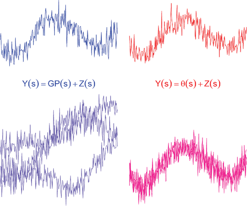
An instance of the choice mentioned in (1) concerns modeling the spatial variability of the mass fraction of uranium in Colorado, considered below, either as a local regression on the geographical coordinates with independent, identically distributed errors or as a Gaussian process. Figure 1 shows sample paths of two very different Gaussian processes on the real line whose true natures one cannot begin to differentiate unless multiple realizations are available.

Figure 1. Heterogeneity vs. interaction. The top row shows single realizations of two very different processes that are practically indistinguishable: on the left, a Gaussian process (GP) with superimposed white noise (Z); on the right, a deterministic signal with superimposed white noise. The bottom row shows three realizations of the same processes, which provide clues as to their true nature.

The fact that first-order (means) and second-order (covariances) moments may be insufficient to capture sensible aspects of spatial phenomena contradicts early beliefs to the contrary, originating in the work of Julesz (1962). Interestingly, it was also Julesz et al. (1973) who discovered patterns that look different yet have the same first- and second-order moments. Figure 2 shows an example based on a binary process discussed in the section on Verhagen model, and Figure 3 shows another. These facts attest to the richness possible in spatial interactions.

Figure 2. Realizations of two versions of Verhagen’s model (Verhagen 1977) that have the same first-order and second-order moments yet are sensibly different.

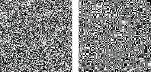
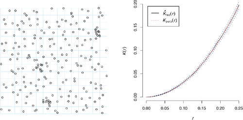
Figure 3. Cell point process (left panel) (Baddeley 2010, Section 19.7), originally defined by Baddeley and Silverman (1984), has the same second-order properties (K-function, right panel) as a homogeneous Poisson point process. A realization of the cell point process is generated by dividing the plane into identical square tiles and scattering, uniformly at random, 0, 1, or 10 points in each, with probabilities 1/10, 8/9, and 1/90, respectively, independently for different tiles. The estimate of the K-function includes the isotropic border correction and is accompanied by an approximate 95% confidence band (dotted lines) (Ripley 1988).

There is a plethora of computational tools to analyze and model spatial data. The treatment of the examples discussed in this article involved facilities from at least the following packages for the R environment for statistical computing and graphics (R Core Team 2015): locfit, mgcv, geoR, gstat, intamap, LatticeKrig, sgeostat, spatial, splancs, spatstat, alphahull, and alphashape3d.

This abundance of riches implies that the user often will have several alternative ways to achieve the same goals: choosing among them implicitly involves model selection. Such selection also involves the tacit acceptance of default settings that the user may not care to optimize for each application but that are influential upon the results.

The following sections present several examples of the analysis of spatial point processes, maps, and shapes, without attempting to be comprehensive in any way, aiming only to illustrate the richness of the field. With few and minor exceptions, none of the analyses or considerations are new or my own, even if I should have fallen short of giving the full and explicit credit to their original authors. Those few and minor contributions that reflect my work include the heuristic interpretation of Dobrushin’s uniqueness theorem for a Markov random field, the analysis of oil wells in Crawford County, Pennsylvania, and the representation of surface structure using α-shapes.

Marks

A point process is a stochastic mechanism that scatters points (also referred to as particles) throughout some space (which will be the Euclidean plane or the surface of a sphere in the examples we will examine), so that each bounded set receives only finitely many points. When, associated with each such point, there is an object that may have been selected at random from a set of marks, then we have a marked point process.

If the space aforementioned is a regular lattice (say, the set of locations on the plane whose coordinates are integer) and each site on the lattice has either 0 or 1 particle, then the point process is a lattice gas, of which the following subsection discusses two examples. If particles may land anywhere on the Euclidean plane, then the point process is a purely atomic random measure (Grandell 1977; Møller and Waagepetersen 2007).

Lattice gases

A lattice gas model is a collection of binary random variables {X_s} indexed by the points of the Euclidean plane with integer coordinates s = (i, j). X_s = 1 indicates that site s is occupied by one particle, and X_s = 0 indicates that it is vacant. The examples we will focus on are the Ising model for a lattice gas, and Verhagen’s model.

Ising model

The probability distribution of the Isingmodel for a lattice gas {X_s} is obtained from the probability distribution of the Ising model for a ferromagnetic collection of interacting spins {Y_s} on the same lattice (McCoy and Wu 1973), by the change of variables Y_s = 2X_s − 1, where each Y_s is either +1 or −1.

For the finite square lattice S_n = {(i, j): 1 ≤ i, j ≤ n}, this is a discrete distribution with probability density p_{α, β}(x) = exp (αU(x) + βV(x))/Z(α, β), for binary configurations , where U(x) is the number of sites of S_n that are occupied and V(x) is the number of pairs of nearest-neighboring sites that are both occupied. If β < 0 then neighbors of sites that are occupied tend to be vacant, and β > 0 induces clustering, while β = 0 corresponds to a Bernoulli process: independent, identically distributed random variables with . Figure 4 shows three realizations of this model on S₁₂₈, with sites (not shown) surrounding the boundary all set to zero for different combinations of values of the parameters.

Figure 4. Realizations of three versions of the Ising lattice gas model on a 128 × 128 lattice, with boundary sites all set to zero and (left panel) α = 3.6 and β = −1.8, (center panel) α = β = 0, and (right panel) α = 3.6 and β = 1.8. The realization in the right panel corresponds to conditions of phase transition.

LaBella et al. (2001) have shown that, its simplicity notwithstanding, the two-dimensional Ising lattice gas model can describe accurately the behavior of a natural system of interacting particles: in particular, of how atoms on a single surface of a crystal of gallium arsenide can be exchanged with the substrate in a reversible manner.

The Ising model was studied by Ernst Ising in the 1920s, following a suggestion from Wilhelm Lenz, his adviser at the University of Hamburg. The closed-form evaluation of the probability density of the Ising model, in the special case where α + 2β = 0 (which in the spin model of ferromagnetism corresponds to the absence of an external magnetic field), was achieved only much later by Onsager (1944), who determined that when and α + 2β = 0, and as the lattice S_n expands as n grows to infinity, the system displays long-range order (a phase transition). This behavior impacts the asymptotic distribution of the sufficient statistics (Pickard 1976, 1977a, 1979).

Even though this orderliness truly happens only for an infinite system, already for a lattice as small as is shown in Figure 4 the manifestation of critical behavior is obvious, with long-range correlations between sites leading to the formation of “continents” of sites that are mostly occupied, separated by “seas” of sites that are mostly vacant. These long-range correlations imply that the boundary conditions (that is, the configuration of the sites that are not in S_n but are nearest-neighbors of the sites along the “edges” of S_n) have a pervasive effect and are never quite “forgotten” as the lattice expands.

Dobrushin’s theorem

Different from the conventional approach to the specification of the joint distribution of a stochastic process via finite-dimensional distributions that satisfy the conditions of Kolmogorov’s existence (or extension) theorem (Kolmogorov 1933; Kallenberg 2002), it is often more convenient to build spatial processes using local conditional distributions, particularly for the important case of Markov processes.

This is already implicitin the definition given above for the probability distribution of the Ising lattice gas on a finite square lattice S_n, because the definition of the aforementioned sufficient statistic V(x), which counts the number of pairs of nearest-neighboring sites that are both occupied, presumes some convention about the boundary conditions (free, toroidal, periodic, etc.); that is, about the occupancy of the sites that “surround” S_n.

The single-site, local conditional distributions for the Ising lattice gas are of the form for s ∈ S_n, where denotes the set of the nearest neighbors of s, and w_s(y) denotes the number of nearest neighbors of s that are occupied in configuration y in the neighborhood of s (which in this case comprises the four sites that are nearest neighbors of s).

In general, a local conditional specification is a family of mutually consistent conditional distributions Q(X_I = x_I|X_{S − I} = x_{S − I}) for I ⊂ S, x_I ∈ {0, 1}^I, and x_{S − I} ∈ {0, 1}^{S − I}. Given such specification, the Vasershtein (1969) distance gauges the extent to which the conditional distribution of X_s is influenced by the value of the conditioning configuration at a site t by measuring how much the conditional distribution of X_s changes when site t “flips” between being vacant or occupied, everything else remaining constant.

The lattice gas is said to be weakly interacting if its conditional specification is such that ∑_{t ∈ S}ρ_st < 1 for each s ∈ S. The counterpart of Kolmogorov’s existence theorem is the following result established by Dobrushin (1968): the conditional specification of a weakly interacting, binary random field on a countable set S defines a unique mixing probability distribution on the space of binary configurations on S.

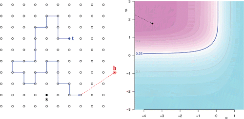
Figure 5 provides a heuristic interpretation of this result and also shows the region of the parameter space for which there is mixing, based on the fact that for the Ising lattice gas ρ_st = max _{k = 0, 1, 2, 3}{|1/(1 + exp {α + βk}) − 1/(1 + exp {α + β(k + 1)})|}, and Dobrushin’s condition reduces to ρ_st < 1/4.

Figure 5. Left panel: For a heuristic interpretation of the existence theorem established by Dobrushin (1968), adjoin a fictitious site (hole) h to S, and define S^* = S∪{h}, ρ_sh = 1 − ∑_{t ∈ S}ρ_st, and ρ_hh = 1. In these circumstances, {ρ_st: s, t ∈ S^*} is the transition matrix of a random walk on S^*, with h as absorbing state that is accessible in a single jump from every site in S; otherwise, jumps are allowed only between neighboring sites. A random walker, starting at t, carries a “message” about changes in value of the configuration there to other sites it visits. If the interaction is weak, the farther t is from s the more likely the walker is to fall into h, and the “message” never reaches s. Right panel: Map of ρ_st(α, β). Dobrushin’s condition suggests criticality when (α, β) lies above and to the left of the 0.25 contour line. This suggestion is conservative when α + 2β = 0 because in this case criticality obtains only once (α, β) is over the dashed segment starting at the black dot.

And if the processis finite-range Markovian, then mixing occurs at an exponential rate, which means that for each finite I ⊂ S, and each finite J ⊂ S disjoint from I, for some γ > 0, and where d(I, J) denotes the distance between sets I and J (for example, the minimum of the distances between sites of one and the other). When there is mixing at exponential rates, then central limit theorems can be proved for functionals of the process (Deo 1975; Bolthausen 1982).

Verhagen model

Verhagen (1977) described a very interesting model for a lattice gas that admits the unilateral construction described in the left panel of Figure 6 yet is homogeneous and Markov (Pickard 1977b). Homogeneity means that if τ is a rigid motion (translation, rotation, reflection) and I ⊂ S_n is such that τ(I) ⊂ S_n, then X_I and X_τ(I) have the same distribution. The Markov property in this case means that the conditional distribution of X_s, given the configuration at all of the other sites of S_n, depends only on the configuration at eight nearest or next-nearest neighbors of s. Owing to the Markov-Gibbs equivalence, , where the sufficient statistics are defined in the right panel of Figure 6.

Figure 6. Left panel: Given a joint distribution Q for (X_{1, 1}, X_{2, 1}, X_{1, 2}, X_{2, 2}) that is invariant under all symmetries of S₂ and such that X_{1, 2} and X_{2, 1} are conditionally independent given X_{1, 1}, the process is constructed considering that the conditional distribution of X_{i, j} (site (i, j) is indicated by the black dot) given the configuration on predecessors of (i, j) (sites within the polygonal outline) depends only on x_{i − 1, j − 1}, x_{i, j − 1}, x_{i − 1, j} (marked with diamonds). Other panels: The sufficient statistics {T_j(x)} count the numbers of clans of sites that are fully occupied. Clans , , and involve only sites on the boundary of S_n.

The distribution Q defined in the caption of Figure 6 may be parameterized in terms of , , and . Since its moments depend only on two of its three parameters, it follows that Verhagen’s model comprises many different distributions with the same second-order structure (Figure 2).

Estimation

Since the natural parameters λ₁,…, λ₈ of the Gibbs distribution of Verhagen’s lattice gas are functions of the three underlying parameters θ, α, and δ aforementioned, the maximum likelihood estimates (MLEs) are the solutions of the following three equations in three unknowns, where for j = 1, …, 8 can all be computed explicitly.

The possibility of computing the MLE in this simple fashion is the exception rather than the rule. Maximum pseudo-likelihood estimation (MPLE), introduced by Besag (1975), is generally practicable for Markov lattice gases and amounts to determining values of the parameters that, in the case of the Ising lattice gas, maximize .

Alternatively, the MLE can be computed using Markov chain Monte Carlo sampling (MCMLE; Geyer 1991). In general, MPLE is much cheaper computationally than MCMLE, but the estimates have greater variability, and MCMLE increasingly outperforms MPLE as the strength of the interaction (β) increases. van Duijn, Gile, and Handcock (2009) also have confirmed the superiority of the MLE over the MPLE for exponential family random graph models that are used to model social networks.

Point processes

When the space S where the stochastic mechanism scatters particles is a continuum (say, the Euclidean plane), point processes are modeled as random variables whose values are nonnegative, integer-valued measures that are finite on bounded subsets of S—these measures indicate where the particles are.

A point process η is completely random if η(B₁), …, η(B_n) are independent when B₁, …, B_n are disjoint and bounded subsets of S. Prékopa (1958) has shown that every (simple and atomless) completely random point process is Poisson; that is, there exists a measure λ such that η(B₁), …, η(B_n) have Poisson distributions with finite means λ(B₁), …, λ(B_n). (Simple means that it places no more than one particle at any location, and atomless that there is no location where it puts a particle with positive probability.)

Prékopa's (1958) characterization that point processes describing interactions must be other than Poisson and suggests that Poisson processes are a natural reference against which to compare more general point processes. Realizations of homogeneous Poisson processes (those whose intensity measure λ is proportional to Lebesgue measure) often appear clustered, and their particles are not evenly distributed in space: this is so because in a Poisson process it is as if particles are completely oblivious to the presence or absence of other particles nearby. Particles will be fairly regularly distributed only if they avoid landing near each other, which contradicts complete randomness.

Oil wells

Figure 7 shows the locations of oil wells in a region of Crawford County, Pennsylvania, each marked with a circle that indicates the volume of oil produced in 2013, which ranged from 15 to 9,470 barrels of oil (2.4 × 10³ L to 1.5 × 10⁶ L), as reported by the Oil and Gas Reporting Website of the Pennsylvania Department of Environmental Protection (https://www.paoilandgasreporting.state.pa.us/publicreports/Modules/Production/ProductionByCounty.aspx, retrieved April 26, 2015).

Figure 7. Locations of oil wells in a region of Crawford County, Pennsylvania, marked with circles that indicate the volumes of oil produced in 2013. The coordinates of the wells have been converted from longitude and latitude to Easting and Northing in a Lambert conic-conformal projection centered at longitude 80.3° west and with reference parallels 41.51° north and 41.80° north.

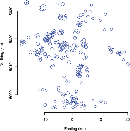
Questions that may be asked about these wells include (1) whether well locations are clustered in space and (2) whether there is a relation between spatial location and productivity. R packages spatstat (Baddeley and Turner 2005; Baddeley, Rubak, and Turner 2015) and splancs (Rowlingson and Diggle 2015) offer many exploratory data analysis tools that help answer these and many other questions about spatial point processes.

Figure 8 suggests that the wells are most concentrated in two areas and that generally they tend to be more clustered than would be expected for a homogeneous Poisson process, except that at very short distances they avoid each other (for example, for values of the interparticle distance r around 0.25 km, the nearest-neighbor cumulative distribution function G(r) dips below its counterpart for the Poisson process). However, the presence of a well does not seem to affect the presence of any other if they are more than 3 km apart.

Figure 8. Left panel: Density of the intensity measure that expresses average number of wells per unit of area. Center panel: Kaplan-Meier estimate of the cumulative probability distribution function of the distance D_s from a particle at s to its nearest neighbor, (solid [blue] line), and its counterpart for a Poisson process, G_pois(r) = 1 − exp (− λπr²) (dashed [red] line). Right panel: Pair correlation function g(r) = K′(r)/(2πr), where K′ is the derivative of Ripley’s K function such that μK(r) is the expected number of further particles within r of a particle and μ is the average number of particles per unit of area (for a homogeneous Poisson process K(r) = πr² and g(r) = 1). Therefore, g(r) is the ratio of the rate at which the number of particles within r of a further particle increases and the corresponding rate for a homogeneous Poisson process: g(r) < 1 suggests inhibition between particles r apart, and g(r) > 1 suggests clustering.

Figure 9 depicts aspects of the relationship between well location and productivity by considering the logarithm of the volume of oil produced as a mark associated with the location of each well. The correlation coefficient between the marks of nearest-neighboring wells is 0.57: a permutation test (Chihara and Hesterberg 2011) shows that it is significantly larger than 0. In particular, the figure shows how the size of the marks varies across the region, the mark correlation function that characterizes how the marks vary together depending on the distance between the particles they are associated with and a generalization of the K function (second-order structure) where the contribution of each pair of particles is weighted by the product of the values of the marks associated with them.

Figure 9. Left panel: Smooth map of the mean value of the marks (base 10 logarithm of the number of barrels of oil produced in 2013) and corresponding standard deviation (dashed contour lines). Center panel: Mark correlation function (solid [blue] line) (Stoyan and Stoyan 1994), where denotes the conditional expectation given that there are particles at locations s and t separated by a distance r, M(s) and M(t) denote the values of the marks attached to them, and M denotes the value of a mark drawn from the marginal distribution of the marks. k_f(r) is not really a “correlation” and it can take any nonnegative value. k_f(r) = 1 (dashed [red] line) obtains when the marks attached to the particles are independent and identically distributed. Right panel: K_f(r) (solid [blue] line) is the mark-weighted K function (Penttinen, Stoyan, and Henttonen 1992), which generalizes Ripley’s K function by weighing the contribution from each pair of particles with a weight proportional to the product of the values of the marks associated with them. The dashed (red) line corresponds to a homogeneous, marked Poisson process where the marks are a sample from their marginal distribution and are independently assigned to the particles.

Measuring finite strain

The raw materials of many of the rocks that we see today, often contorted into spectacular folds (Figure 10), were originally deposited in essentially horizontal layers, either at the bottom of seas and lagoons or on land, after transport by water or by wind. These materials eventually hardened into rocks as later sediments buried them and were compressed and deformed during collisions between continents, eventually being uplifted into mountains like the Alps or the Andes, only for the cycle to begin anew, that will weather them into a new generation of raw materials for the mountains of tomorrow—a process repeated many times already since the Earth was new (Prothero and Dott 2009).

Figure 10. Left panel: Folded limestones from the Jurassic Coast (Stair Hole, Lulworth Cove, Dorset, UK), originally deposited as horizontal sedimentary layers at the bottom of coastal lagoons and swamps about 135 million years ago. The mountain building processes that deformed and uplifted them were part of the Alpine orogeny and occurred about 50 million years ago (Geological Society of London 2015). Image copyright 2015 ScienceStockPhotos (Creative Commons Attribution 4.0 International), from http://sciencestockphotos.com/free/geology/slides/folded_sedimentary_layers.html. Right panel: Locally, deformation is approximately affine: circles become ellipses all with the same shape as the strain ellipse.

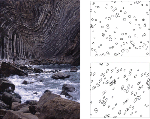
Although large-scale deformation as shown in Figure 10 is nonlinear, locally it may be approximately linear. Therefore, if the rock contained approximately spherical objects before deformation, after deformation they will be approximately ellipsoidal. Many different objects of nonspherical initial shape may also be used as strain markers, either individually or in groups; that is, they provide sufficient information to allow estimating the axial ratio and orientation of the axes of the ellipsoid (or ellipse, in 2D) that a sphere would be transformed into by locally linear finite strain (Ramsay and Huber 1983).

The left panel of Figure 11 shows the locations of centers of ooids in an oolite (Ramsay and Huber 1983, figure 7.7), which is a sedimentary rock composed of approximately spherical particles (typically consisting of multiple concentric layers) embedded in a matrix. If the mechanical properties of the ooids and of the matrix they are embedded in are different, then the ellipsoids that the ooids become as a result of finite strain provide biased estimates of the total strain the rock has undergone. However, the point process whose points are the centers of the ooids can be used as a strain marker.

Figure 11. Left panel: Locations of centers of ooids in a photomicrograph of an oolite (Ramsay and Huber 1983, figure 7.7), whose coordinates are provided as an example input file for EllipseFit (Vollmer 2015). Center panel: Fry plot (magnified) produced by function fryplot defined in R package spatstat (Baddeley and Turner 2005; Baddeley, Rubak, and Turner 2015). The ellipse fitted to the densest “ridge” surrounding the central conditioning location, is an estimate of the strain ellipse. Right panel: Simulation produced using Strauss hard-core model fitted to the data on the left panel, after “unstraining,” as described in the text. The (red) circle illustrates the interaction distance , and the (red) dot inside that circle illustrates the hard-core of radius .

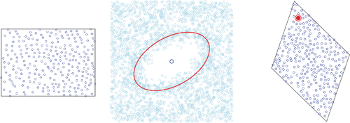
The idea, which Fry (1979) developed into a practicable method for strain estimation, is the following: if the point process is isotropic and otherwise such that the presence of a particle tends to inhibit the presence of other particles nearby, then the empty space around a typical particle acts as a “virtual” circular marker that becomes elliptical in the strained condition.

The informative attribute of the process is the intensity (expected value measure) of the conditional distribution of the process given that it has a particle at the origin (of the coordinates). The center panel of Figure 11 shows the process conditioned to have a particle at the origin (the center of the plot): the number of particles per unit of area is an estimate of the aforementioned conditional intensity measure. The ellipse fitted to the densest “ridge” is an estimate of the strain ellipse: it has axial ratio 1.7 and major axis at 30 ° from the horizontal axis.

Modeling

The point pattern displayed in the left panel of Figure 11 may possibly be modeled with a Strauss hard core model, which generally models inhibition or repulsion between neighboring particles, with the added constraint that no two particles may be closer together than a minimum distance. However, it is easier to fit such model after “unstraining” the pattern by applying to it a linear transformation that converts the estimated strain ellipse into a circle.

Baddeley (2010, Section 26.1) provides a general definition for the probability density of a point process. The Strauss hard core model has probability density f(x) = 0 when any two points are less than h > 0 apart, and f(x) = αβ^n(x)γ^s(x), where x denotes the set of locations of the particles of the process, n(x) is the number of particles within the sampling window, and s(x) is the number of pairs of points that are within r of each other. If γ < 1, then the presence of a particle at a particular location tends to inhibit the presence of other particles nearby.

This model may be fitted to the ooid centers (after “unstraining,” as described above) by maximum pseudo-likelihood estimation or the one-step approximation to maximum likelihood suggested by Huang and Ogata (1999), as implemented in R function ppm defined in R package spatstat (Baddeley and Turner 2005; Baddeley, Rubak, and Turner 2015). The hard-core range h is estimated by the minimum nearest neighbor distance multiplied by n(x)/(n(x) + 1). The range parameter r is estimated by maximum profile pseudolikelihood (Baddeley 2010, Section 26.1). For this data set, using the method suggested by Huang and Ogata (1999) and Ripley’s correction for boundary effects, we obtained (which confirms the inhibitory nature of the process), interaction distance , and hard-core radius . The right panel of Figure 11 shows a realization from this fitted model.

Maps

Maps depict the spatial variability of the values of a property as a function of the geographical coordinates. The maps we will consider in this section summarize measurements of radioactivity around Fukushima, Japan (Section 3.1), and of abundances of several chemical elements in geochemical surveys, uranium in Colorado, and titanium and thorium in the eastern seaboard of the United States.

Radioactivity in Fukushima

On March 11, 2011, sea waves raised by the magnitude 9.0 (M_w) Great East Japan earthquake over-topped the sea wall protecting the Fukushima Daiichi nuclear power plant, causing loss of power and also damaging backup generators, leading to the worst nuclear disaster since Chernobyl, which happened 25 years earlier.

Figure 12shows two maps derived from the same set of measurements of radioactivity made by Safecast during September 2011 in the region of Fukushima. Safecast is “a global project to empower people with data, primarily by mapping radiation levels and building a sensor network, enabling people to contribute and freely use the data collected” (http://blog.safecast.org/).

Figure 12. Left panel: Robust, locally quadratic regression implemented in R package locfit (Loader 1999, 2013). Right panel: Kriging interpolant implemented in R package intamap (Pebesma et al. 2010). The units of the labels of the contour lines are milliroentgen per hour (1 mR = 2.58 × 10⁻⁷ C/kg). The black dots near the top and right edges of the maps indicate the locations of the city of Fukushima and of the Fukushima Daiichi nuclear power plant, respectively.

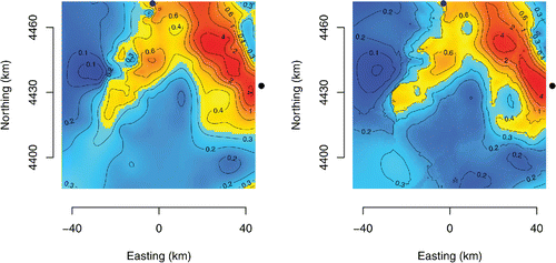
Both maps (Figure 12) involve interpolating measurements made at a discrete set of locations (a sample of 1,250 locations drawn from the set of almost 123,000 locations where a measurement was made). The interpolants were (1) a robust, locally quadratic regression (Loader 1999) implemented in R package locfit (Loader 2013), and (2) a kriging interpolant (Diggle and Ribeiro 2010) implemented in R package intamap (Pebesma et al. 2010).

Both the locally quadratic regression and the kriging interpolant were fitted to the measured values of radioactivity after applying a Box-Cox transformation that brings the marginal distribution of the transformed values closer to a Gaussian distribution and stabilizes the variance (Box and Cox 1964). The power λ = −0.42 was selected using function boxcox defined in R package MASS (Venables and Ripley 2002).

Listing 1 illustrates how intamap facilitates fitting a flexible kriging model (Gaussian process with Matérn’s covariance function; Matérn 1987; Stein 1999), taking any anisotropy into account. These facilities are an output of Interoperability and Automated Mapping, a 2006–2009 project funded by the European Commission used for near real-time mapping of gamma-ray dose rates across Europe.

require(intamap)  nx = ny = 900  x = seq(from=min(rad$x), to=max(rad$x), by=ny)  y = seq(from=min(rad$y), to=max(rad$y), by=nx)  xy = expand.grid(x=x, y=y)  coordinates(rad) = x+y  coordinates(xy) = x+y  kObj = createIntamapObject(            observations = rad,          formulaString=as.formula(z1),          predictionLocations=xy,            class = ''automap'',            ouputWhat = list(mean=TRUE, variance=TRUE),            params = list(doAnisotropy=TRUE, nmax=50))  checkSetup(kObj)  kObj = preProcess(kObj)  kObj = estimateAnisotropy(kObj)  kObj = estimateParameters(kObj)  kObj = spatialPredict(kObj)  kObj = postProcess(kObj)  zGRID = array(kObj$outputTable[,''mean''], dim=c(nx,ny)) LISTING 1. R code for “automatic” kriging using package intamap, assuming that dataframe rad has geographical coordinates in x and y and the Box-Cox transformed readings of radioactivity in z.

Cross-validation (Mosteller and Tukey 1977) is a reliable procedure to evaluate the accuracy of a predictor. In a spatial context, it needs to be applied considering the structure of the sampling locations. The measurements of radioactivity in the region of Fukushima following the nuclear disaster were made by volunteers using portable detectors, mostly along roads, as may be inferred from inspection of the left panel of Figure 13.

Figure 13. Left panel: Measurement locations marked by dots of the same hue are examples of subsets of measurement locations to be left out to assess prediction accuracy via cross-validation. Right panel: Comparison of kriging and local regression prediction “errors” (differences between predicted and observed values in measurement units that correspond to the Box-Cox transformation of milliroentgen per hour with exponent λ = −0.42).

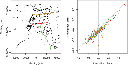
The principal challenge that the interpolants face consists of filling the large gaps between roads. Therefore, cross-validation ought to proceed by leaving out whole strings of measurements along individual roads, as indicated using different colors in the same panel of the same figure. The right panel shows differences between predicted and observed values that estimate the cross-validated prediction errors and also suggests that, albeit different in detail, both the local regression and the kriging interpolants perform comparably well.

Uranium in Colorado

The National Geochemical Survey maintained by the U.S. Geological Survey (U.S. Geological Survey Open-File Report 2004-1001, version 5.0 available at http://mrdata.usgs.gov/geochem/doc/home.htm, accessed March 22, 2015) includes data for 1,150 samples, primarily of stream sediments, collected in Colorado between 1975 and 1980 as part of the National Uranium Resource Evaluation (NURE) program (Smith 2001). The corresponding data may be downloaded (in any one of several formats) from http://mrdata.usgs.gov/geochem/select.php?place=fUS08&div=fips.

The mass fraction of uranium in these samples was measured using delayed neutron counting (Knight and McKown 2002). The measured values range from 1 to 147 mg/kg, and their distribution is markedly asymmetric, with right tail much longer than the left. A Box-Cox transformation with λ = −0.7 reduces such asymmetry substantially, and generally makes a Gaussian model more plausible.

The measurand is the function θ that, given the geographical coordinates (u, v) of a location within Colorado, produces an estimate of the mass fraction of uranium in sediments at that location. The generic model expresses the measured value of the mass fraction of uranium w(u, v) as (w(u, v)^λ − 1)/λ = θ(u, v) + ε(u, v).

The measurement errors {ε(u, v)} are assumed to behave like values of independent, Gaussian random variables with mean zero and the same standard deviation. The function θ is deterministic in two of the models considered below and stochastic in two others.

A polynomial (in the geographical coordinates) would be an example of a deterministic function. A collection of correlated Gaussian random variables, where each one describes the mass fraction of uranium at one location in the region, would be an example of a stochastic function. The correlations capture the fact that neighboring locations tend to have more similar values of mass fraction than locations that are far apart.

Figure 14 shows that both deterministic and stochastic functions can model very much the same patterns in the spatial variability of the data. Even though the function θ can be evaluated at any location throughout the region, here it is displayed as an image that depicts the values of θ at the center of each pixel in a regular grid comprising 40 × 30 pixels. These are the four models used for θ:

Figure 14. Four estimates of the spatial distribution of the mass fraction of uranium in stream sediments throughout Colorado: (1) Q (locally quadratic regression, top left); (2) K (ordinary kriging, top right); (3) G (generalized additive model, bottom left); and (4) L (multiresolution Gaussian process model, bottom right). The black square marks the location of the city of Denver, and the small dots mark the locations that were sampled. The geographical coordinates are expressed in kilometers, and the labels of the contour lines are expressed in milligrams per kilograms.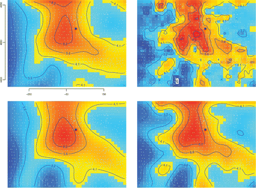

Q:	Locally quadratic regression model with nearest-neighbor component of the smoothing parameter chosen by cross-validation, as implemented in R package locfit (Loader 1999, 2013);
K:	Ordinary kriging model with Matérn’s covariance function and estimation of spatial anisotropy as implemented in R package intamap (Stein 1999; Pebesma et al. 2010);
G:	Generalized additive model with thin-plate regression splines and smoothing parameter chosen by generalized cross-validation, as implemented in R package mgcv (Wood 2003, 2006);
L:	Multiresolution Gaussian process model as implemented in R package LatticeKrig, with default settings for all the user adjustable parameters (Nychka et al. 2013, 2014).

The four estimates of θ are generally similar but clearly differ in many details. (Obviously, other models could also be reasonably entertained.) The significance of these differences depends on the uncertainty associated with each estimate. Instead of exploring the differences when evaluating uncertainty, one may choose instead to combine the estimates and then to capture the differences that are attributable to model uncertainty alongside other identifiable sources of uncertainty.

Model averaging is often used for this purpose (Hoeting et al. 1999; Clyde and George 2004), which typically is done by computing the weighted mean of the results corresponding to the different models, with weights proportional to the Bayesian posterior probabilities of the models given the data.

In this case, we adopt the simplest version possible of model averaging, which assigns to the pixel with center coordinates (u, v) the (unweighted) arithmetic average of the values that the four estimates described above take at this location: .

Figure 15shows this pixelwise average and also the endpoints of pixelwise probability intervals for θ (one interval at each of the pixels in the image) based on a Monte Carlo sample of size K = 1, 000 drawn from the probability distribution of θ. Each element in this sample, for k = 1, …, K, is a map built as follows, where m = 1, 150 denotes the number of locations where the mass fraction of uranium was measured:

Figure 15. The center panel shows the pointwise average of the four estimates of the spatial distribution of the mass fraction of uranium depicted in Figure 14. The black dot marks the location of the city of Denver, and the small dots mark the locations that were sampled. The geographical coordinates are expressed in kilometers, and the labels of the contour lines are expressed in milligrams per kilograms. The left and right panels show the left and right end-points of approximate 95% probability intervals for θ.

(1)	Draw a sample of size m, uniformly at random and with replacement, from the set of m locations where sediment was collected for analysis,
(2)	Since the same location may be selected more than once, the geographical coordinates of all of the locations that are drawn into the sample are jittered slightly, to avoid the occurrence of duplicated locations, which some of the software used cannot cope with,
(3)	Obtain estimates , , , as described above but using the sample drawn from the original data,
(4)	Compute .

The probability interval at the pixel whose center has coordinates (u, v) has left and right endpoints equal to the 2.5th and 97.5th percentiles of . These maps of percentiles indicate how much, or how little, of the structures apparent in are significant once measurement uncertainty is taken into account.

Contextual imputation of non-detects and missing values

In geochemical surveys, samples are often measured where the value of the measurand (typically the mass fraction of a particular chemical element) is found to be below the detection limit of the instrument used for measurement. Since knowing an upper bound for the property of interest at a particular location obviously is informative about the spatial variability of this property, the nondetects should contribute to geochemical mapping.

When the nondetects are a fairly small proportion of the data, it may be possible to impute them using the spatial context in which they occur, taking into account the upper bound on their value, thereby producing a more informative map than if nondetects were simply discarded.

We illustrate how this may be done using measurements of the mass fractions of titanium and thorium made on 834 samples collected in an area of the Eastern United States (data from the National Geochemical Survey, kindly compiled and shared by Dr. Andrew Grosz of the U.S. Geological Survey). For 156 of these samples the mass fraction of thorium is below the corresponding detection limit (6 mg/kg). The goal is to map the ratio of mass fractions of titanium (for which there are no missing data) and thorium, which we denote informally by Ti/Th.

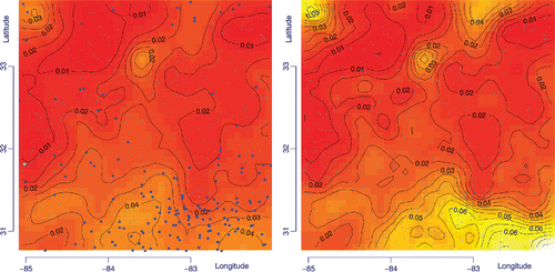
The ratios at those 156 locations are said to be (right) censored because all that one knows about them is that they are greater than (lie to the “right” of) Ti/6. To impute them we develop a geostatistical model for the spatial variability of Ti/Th, first using only the complete data. Next, we use the fitted model to estimate Ti/Th at each location where it is censored. This estimate is the conditional expectation of the value of the ratio that the model predicts for that location, given that the ratio should exceed the lower bound for that location. Afterward we repeat these two steps in alternation (model fitting using also the imputed values as if they were observed data, and updating of that conditional expectation) until the imputed values and the map itself stabilize (Figure 16).

Figure 16. Maps of the ratio of the mass fractions of titanium and thorium (Ti/Th). Left panel: Interpolation done using only the complete (uncensored) data and a Gaussian process model (and kriging estimate), with a powered exponential covariance function, fitted to log (Ti/Th) using facilities available in R package geoR (Ribeiro and Diggle 2001; Diggle and Ribeiro 2010). Right panel: Corresponding map built using the data after imputation of the right-censored observations.

Shapes

The Cambridge Dictionaries Online (2015) define shape as “the particular way something looks as a whole” and the 9th edition of the dictionary of the Académie Française (2015) defines forme as “Aspect extérieur, configuration caractéristique ou particulière.”

Shape has been recognized as an important attribute since long ago: “I doubt not but if we could discover the figure, size, texture, and motion of the minute constituent parts of any two bodies, we should know without trial several of their operations one upon another, as we do now the properties of a square, or a triangle” (Locke [1960] 1975, Book IV, Chapter III, Section 25). Shape is a key functional attribute of: cells in biological tissues, grains in industrial mineral powders (including cement), proteins in blood, carbon nanotubes in polymers, and parts in industrial machinery or in the human body.

Shape representation

The measurement of shape (shape metrology) involves the representation of shape and then the determination of the values of the constituent elements of this representation, suitably qualified with evaluations of the associated uncertainty. Particularly useful shape representations include collections of landmarks (Dryden and Mardia 1998; Lele and Richtsmeier 2001), deformable templates (Grenander and Miller 2007), level sets and active contours (Sethian 1999; Osher and Fedkiw 2003), and α-convex hulls and α-shapes (Edelsbrunner, Kirkpatrick, and Seidel 1983; Pateiro-López and Rodríguez-Casal 2010; Lafarge et al. 2014).

Figure 17 depicts samples drawn from two distributions of Gaussian polygons that are deformed instances of regular polygonal templates (Grenander and Miller 1994).

Figure 17. Samples from two populations (red and blue) of Gaussian polygons. Each polygon is an affine transformation of an underlying template, a regular polygon with a given number of sides and one vertex at the origin of the reference frame. The affine transformations involve a shift and a linear transformation, which may be parameterized in such a way that selecting a transformation at random is equivalent to making a drawing from a multivariate Gaussian distribution.

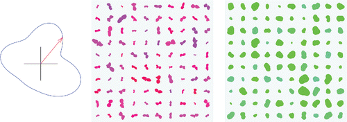
Figure 18 shows samples drawn from two distributions of star-shaped objects using the radial representation suggested by Hobolth, Pedersen, and Jensen (2003). A 2D star-shaped object is a closed, connected subset of the Euclidean plane for which there exists an interior point (“center”) such that the straight line segment connecting this “center” to any point on the boundary of the subset does not intersect the boundary anywhere else.

Figure 18. Left panel: Radial representation for star-shaped objects is based on a truncated Fourier representation of the radius vector that connects the “center” of the object to a point on its boundary, , so that the points on the boundary have Cartesian coordinates (X(t), Y(t)) = (X₀, Y₀) + S R(t)(cos (2πt), sin (2πt)). The parameters c₁ and d₁ define a “base” shape, S, C₂, C₃, … may be modeled as gamma random variables, and D₂, D₃, … as uniformly distributed random variables. Center and right panels: Realizations corresponding to two different sets of parameters for the gamma random variables.

α-convex hulls and α-shapes

The α-convex hull generalizes the concept of convex hull of a set of points. Figure 19 shows both α-convex hulls for the same set of points and two different values of α. Similarly to how the convex hull is characterized (intersection of half-spaces bound by planes tangent to the set), the α-convex hull is the intersection of the complements of open balls of radius α > 0 that do not intersect the set (what is left if carving out all the space with a spherical scoop of radius α without removing any of the points in the set; Walther 1997, 1999; Pateiro-López and Rodríguez-Casal 2010; Lafarge et al. 2014).

Figure 19. α-convex hulls of the same set of points corresponding to two different values of the probing radius α, the associated α-shapes, and their “outward” pointing surface normals.

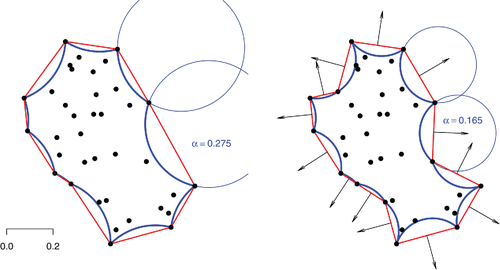
The boundary of the α-convex hull is a union of arcs of circles (in 2D) or of spherical caps (in 3D) and intersections of these elements. If this boundary is approximated by a polygonal curve (in 2D) or by a polyhedral surface (in 3D), the result is yet another approximation to the surface of the set, called the α-shape. Figure 19 shows the α-shapes corresponding to the α-convex hulls and also the “outward” pointing normals of the edges of the α-shapes.

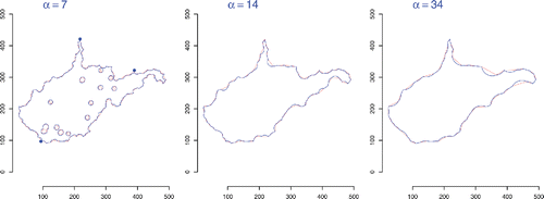
The value of the probing radius α is the scale at which one wishes to explore the structure of the surface of an object in 2D or 3D (Figure 20): small values of the radius allow the α-shape to track the surface closely, while large values lead to an approximation that captures the large features and overall aspect of the shape.

Figure 20. To compute the α-convex hull and α-shape of a bounded region of the plane (or of 3D space)—for example, using the facilities available in R packages alphahull (Pateiro-López and Rodríguez-Casal 2015) and alphashape3d (Lafarge and Pateiro-López 2014)—one draws a sufficiently large sample of points distributed uniformly at random over the region and uses its α-convex hull (or shape) as an estimate of the α-convex hull (or shape) of the region: Rodríguez Casal (2007) describes properties of such estimator.

Surface structure and intrinsic dimension

The α-shape facilitates estimating surface area, quantifying nonconvexity, characterizing the roughness and the local orientation of the surface, and querying the surface in other ways. In particular, it offers the flexibility to study the geometry of the surface at multiple spatial scales, depending on the tuning parameter α.

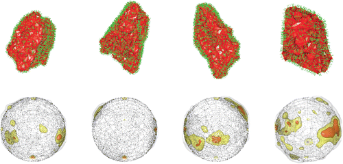
Figure 21 shows particular views of 3D α-shapes of cement particles, built from sets of points that sample the particles densely, using facilities available in R package alphashape3d (Lafarge and Pateiro-López 2014). Grain size, shape, and surface structure in particular, are key drivers of how quickly cement grains will hydrate when mixed with water, thereby determining the time it takes for the mixture to set (Garboczi et al. 2014). The variability of the outward pointing surface normals of the surface elements that comprise the α-shape, captured in probability density estimates on the surface of a sphere, is informative about the general orientation of the main features of the surface of the grains.

Figure 21. Top row: α-shapes and surface normals of cement particles whose shapes have been reconstructed using computed X-ray tomography. Bottom row: Probability density estimates of the orientations of the surface normals.

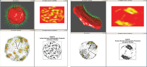
Figure 22 shows how α-shapes and derivative products (stereographic projection of surface normals, probability density of orientations of surface normals, and marked point process on the surface of a sphere indicating the orientation of the surface normals and with marks indicating the areas of the surface elements) may be used to probe the intrinsic dimensionality of an object: for example, whether it is essentially 3D (like a roughly spherical blob) or whether it is intrinsically 2D, even if embedded in 3D (like a thin pancake on a cylindrical surface).

Figure 22. Left panel: For a spherical blob, which is intrinsically 3D, α-shape (top left), probability density of the stereographic projection of surface normals (top right), probability density of orientations of surface normals (bottom left), and marked point process on surface of a sphere indicating the orientation of the surface normals and with marks indicating the areas of the surface elements. Right panel: Corresponding displays for a hyperbolic slab, which is intrinsically 2D.

Figure 23 shows the cloud of points (in 3D) used to sample a polymeric scaffold used for bioengineering applications and a corresponding α-hull. Because the latter is a polyhedral surface, it facilitates the computation of geometric attributes.

Figure 23. Left panel: Point cloud (in 3D) used to sample a polymeric scaffold. Center panel: α-shape derived from the point cloud, revealing a stack of tubular structures. Right panel: Probability density estimate for the tortuosity ratio.

For example, some of these scaffolds are seeded with osteoblasts or other biological cells intended to grow into a structured tissue (say, cartilage for an ear). It is then important to verify that the porosity (fraction of the total volume that is void) and permeability of the structure meets operational requirements for the development of the tissue and for nutrients to reach all of its parts.

Other meaningful attributes are the internal connectivity and tortuosity of the scaffold. Connectivity may be described as the probability that, given two interior points selected uniformly at random within the volume occupied by the scaffold, there will exist an unobstructed path leading from one to the other. Tortuosity quantifies the “wiggliness” of the pathway between two points selected randomly within the structure. It may be characterized by the ratio of two distances between these points: one distance is as the crow flies and the other is along unobstructed pathways within the structure. The right panel of Figure 23 shows a probabiity density estimate for the tortuosity ratio derived from pairs of random points within the structure.

Summation

In many applications, a choice must be made between (1) a model with independent, heterogeneous random components and an underlying, deterministic function that describes the spatial pattern and (2) a model with dependent, homogeneous random components, whose dependence structure describes the spatial pattern. Different choices typically involve different modeling costs.

Cross-validation must be responsive to how the data were acquired and to how the fitted model tracks the data and produces predictions.

Model selection and choice of “default” settings of software used in model-fitting are influential tasks in the statistical arts. Very often they make substantial contributions to the uncertainty of the results, and just about as often these contributions are ignored.

Spatial statistics is both interesting and challenging because it attempts to capture and model the fact that “Everything is related to everything else, but near things are more related than distant things” (Tobler 1970, p. 236).

About the author

Antonio Possolo is a NIST Fellow and the Chief Statistician for NIST (National Institute of Standards and Technology, U.S. Department of Commerce, in Gaithersburg, Maryland). He holds a Ph.D. in statistics from Yale University, where he was a student of John Hartigan’s. His primary focus areas are the evaluation of measurement uncertainty and the application of statistical models and methods in measurement science. He chairs the working group on Statistics and Uncertainty of the Technical Committee of the Sistema Interamericano de Metrologia (SIM) and is a member of the Commission on Isotopic Abundances and Atomic Weights (CIAA) of the International Union of Pure and Applied Chemistry (IUPAC) and of Working Group 1 (GUM) of the Joint Committee for Guides in Metrology at the Bureau International des Poids et Mesures (BIPM).

Acknowledgments

Peter Goos (University of Antwerp, Katholieke Universiteit Leuven) and Roger Hoerl (Union College) honored the author with an invitation to present this material at the 2015 Stu Hunter Research Conference that was held in Leuven, Belgium, March 9–11, 2015, in the Leuven Institute for Ireland in Europe. Denis Allard (INRA, France) and Alfred Stein (University of Twente, The Netherlands) greatly enriched the presentation by leading a thoughtful and valuable discussion of it. Marit Schoonhoven (University of Amsterdam) very kindly oversaw the refereeing and publication of this contribution for this Special Issue with great attention to detail. Andrew Grosz (U. S. Geological Survey) kindly compiled and shared the data from the National Geochemical Survey. Joy Dunkers (Biosystems and Biomaterials Division, Material Measurement Laboratory, NIST) shared the data about the polymeric scaffold used in Figure 23. Thomas Lafarge created the software application CAVOSS3D that uses α-shapes to measure properties of polymeric scaffolds (Dunkers et al. 2013). Adam Pintar and Jolene Splett (Statistical Engineering Division, Information Technology Laboratory, NIST) offered numerous suggestions for improvement. Olha Bodnar (Physikalisch-Technischen Bundesanstalt, Germany) provided inspiration for the sections on Marks and on Shapes.

References

- Académie Française. Dictionnaire de l’Académie française, neuviéme édition, 2015. http://www.academie-francaise.fr/le-dictionnaire. (accessed April 28, 2015).
- Baddeley, A. 2010. Analysing spatial point patterns in R. CSIRO Australia, December 2010.
- Baddeley, A. 2013. Spatial point patterns: Models and statistics. In Stochastic Geometry, Spatial Statistics and Random Fields, number 2068 in Lecture Notes in Mathematics, ed. E. Spodarev, 49–114. Berlin, Germany: Springer-Verlag.
- Baddeley, A., E. Rubak, and R. Turner 2015. Spatial point patterns: Methodology and applications with R. London, UK: Chapman and Hall/CRC Press.
- Baddeley, A. J., and B. W. Silverman 1984. A cautionary example on the use of second-order methods for analyzing point patterns. Biometrics 40:1089–94.
- Baddeley, A., and R. Turner 2005. spatstat: An R package for analyzing spatial point patterns. Journal of Statistical Software 12:1–42. http://www.jstatsoft.org/v12/i06/.
- Besag, J. 1975. Statistical analysis of non-lattice data. Journal of the Royal Statistical Society. Series D (The Statistician) 24 (3):179–95.
- Bolthausen, E. 1982. On the central limit theorem for stationary mixing random fields. The Annals of Probability 10 (4):1047–50.
- Box, G. E. P., and D. R. Cox 1964. An analysis of transformations. Journal of the Royal Statistical Society. Series B (Methodological) 26 (2):211–52.
- Cambridge Dictionaries Online 2015. American English. http://dictionary.cambridge.org (accessed April 28, 2015).
- Chihara, L. M., and T. C. Hesterberg 2011. Mathematical statistics with resampling and R. Hoboken, NJ: John Wiley & Sons.
- Clyde, M., and E. I. George 2004. Model uncertainty. Statistical Science 19:81–94.
- Cressie, N., and C. K. Wikle 2011. Statistics for spatio-temporal data. Hoboken, NJ: John Wiley & Sons.
- Daley, D. J., and D. Vere-Jones 2003a. An introduction to the theory of point processes—Volume I: Elementary theory and methods, 2nd ed. New York, NY: Springer.
- Daley, D. J., and D. Vere-Jones 2003b. An introduction to the theory of point processes—Volume II: General theory and structure, 2nd ed. New York, NY: Springer.
- Deo, C. M. 1975. A functional central limit theorem for stationary random fields. The Annals of Probability 3 (4):708–15.
- Diggle, P. J. 2003. Statistical analysis of spatial point patterns, 2nd ed. London, UK: Arnold.
- Diggle, P. J., and P. J. Ribeiro 2010. Model-based geostatistics. New York, NY: Springer.
- Dobrushin, R. L. 1968. The description of a random field by means of conditional probabilities and conditions of its regularity. Theory of Probability and Its Applications 13:197–224.
- Dryden, I. L., and K. V. Mardia 1998. Statistical shape analysis. Chichester, UK: John Wiley & Sons.
- Dunkers, J. 2013. CAVOSS3D - Computation and Visualization of Scaffold Structure. ASTM Scaffolds Workshop, Indianapolis, IN, May 2013.
- Edelsbrunner, H., D. G. Kirkpatrick, and R. Seidel 1983. On the shape of a set of points in the plane. IEEE Transactions on Information Theory 29:551–59.
- Fry, N. 1979. Random point distributions and strain measurement in rocks. Tectonophysics 60 (1–2):89–105.
- Garboczi, E. J., D. P. Bentz, K. A. Snyder, N. S. Martys, P. E. Stutzman, C. F. Ferraris, and J. W. Bullard 2014. Modeling and measuring the structure and properties of cement-based materials. Gaithersburg, MD: National Institute of Standards and Technology. http://ciks.cbt.nist.gov/monograph/.
- Geological Society of London. The rock cycle (ks3)—Folding, dorset. http://www.geolsoc.org.uk/ks3/gsl/education/resources/rockcycle/page3801.html (accessed April 26, 2015).
- Geyer, C. J. 1991. Markov chain Monte Carlo maximum likelihood. http://www.stat.umn.edu/geyer/f05/8931/c.pdf (accessed November 23, 2015).
- Grandell, J. 1977. Point processes and random measures. Advances in Applied Probability 9 (3):502–26.
- Grenander, U., and M. I. Miller 1994. Representations of knowledge in complex systems. Journal of the Royal Statistical Society 56 (4):549–603.
- Grenander, U., and M. Miller 2007. Pattern theory: From representation to inference. New York, NY: Oxford University Press.
- Hobolth, A., J. Pedersen, and E. B. V. Jensen 2003. A continuous parametric shape model. Annals of the Institute of Statistical Mathematics 55 (2):227–42.
- Hoeting, J. A., D. Madigan, A. E. Raftery, and C. T. Volinsky 1999. Bayesian model averaging: A tutorial. Statistical Science 14 (4):382–417.
- Huang, F., and Y. Ogata 1999. Improvements of the maximum pseudo-likelihood estimators in various spatial statistical models. Journal of Computational and Graphical Statistics 8:510–30.
- Julesz, B. 1962. Visual pattern discrimination. IRE Transactions on Information Theory 8 (2):84–92.
- Julesz, B., E. N. Gilbert, L. A. Shepp, and H. L. Frisch 1973. Inability of humans to discriminate between visual textures that agree in second-order statistics—Revisited. Perception 2:391–405.
- Kallenberg, O. 2002. Foundations of modern probability, 2nd ed. New York, NY: Springer-Verlag.
- Knight, R. J., and D. M. McKown 2002. Uranium and thorium by delayed neutron counting. In Analytical methods for chemical analysis of geologic and othermaterials, U.S. Geological Survey, ed. J. E. Taggart, Z1–Z5. Denver, CO: U.S. Geological Survey, U.S. Department of the Interior.
- Kolmogorov, A. N. 1933. Foundations of the theory of probability, 2nd ed., trans. N. Morrison. New York, NY: Chelsea Publishing Co..
- LaBella, V. P., D. W. Bullock, Z. Ding, C. Emery, A. Venkatesan, W. F. Oliver, G. J. Salamo, P. M. Thibado, and M. Mortazavi 2001. Spatially resolved spin-injection probability for gallium arsenide. Science 292 (5521):1518–21.
- Lafarge, T., and B. Pateiro-López 2014. alphashape3d: Implementation of the 3D alpha-shape for the reconstruction of 3D sets from a point cloud. http://CRAN.R-project.org/package=alphashape3d.
- Lafarge, T., B. Pateiro-López, Antonio Possolo, and J. P. Dunkers 2014. R implementation of a polyhedral approximation to a 3D set of points using the α-shape. Journal of Statistical Software 56.
- Lele, S. R., and J. T. Richtsmeier 2001. An invariant approach to statistical analysis of shapes. Boca Raton, FL: Chapman and Hall/CRC.
- Loader, C. 1999. Local regression and likelihood. New York, NY: Springer-Verlag.
- Loader, C. 2013. locfit: Local regression, likelihood and density estimation. http://CRAN.R-project.org/package=locfit.
- Locke, J. [1690] 1975. An essay concerning human understanding, ed. P. H. Nidditch. Oxford, UK: Oxford University Press.
- Matérn, B. 1987. Spatial variation, 2nd ed. Lecture Notes in Statistics. New York, NY: Springer-Verlag.
- McCoy, B. M., and T. T. Wu 1973. The two-dimensional ising model. Mineola, NY: Dover Publications.
- Møller, J., and R. P. Waagepetersen 2007. Modern statistics for spatial point processes. Scandinavian Journal of Statistics 34 (4):643–84.
- Mosteller, F., and J. W. Tukey 1977. Data analysis and regression. Reading, MA: Addison-Wesley Publishing Company.
- Nychka, D., S. Bandyopadhyay, D. Hammerling, F. Lindgren, and S. Sain 2013. A multi-resolution gaussian process model for the analysis of large spatial data sets. NCAR Technical Note NCAR/TN-504+STR, Boulder, CO: National Center for Atmospheric Research.
- Nychka, D., D. Hammerling, S. Sain, and N. Lenssen 2014. LatticeKrig: Multiresolution kriging based on Markov random fields. http://CRAN.R-project.org/package=LatticeKrig.
- Onsager, L. February 1944. Crystal statistics. I. A two-dimensional model with an order-disorder transition. Physical Review 65:117–49.
- Osher, S., and R. Fedkiw 2003. Level set methods and dynamic implicit surfaces. Number 153 in Applied Mathematical Sciences. New York, NY: Springer-Verlag.
- Pateiro-López, B., and A. Rodríguez-Casal 2010. Generalizing the convex hull of a sample: The R package alphahull. Journal of Statistical Software 34:1–28.
- Pateiro-López, B., and A. Rodríguez-Casal 2015. alphahull: Generalization of the convex hull of a sample of points in the plane. http://CRAN.R-project.org/package=alphahull (accessed November 23, 2015).
- Pebesma, E., D. Cornford, G. Dubois, G. B. M. Heuvelink, D. Hristopoulos, J. Pilz, U. Stoehlker, G. Morin, and J. O. Skoien 2010. INTAMAP: The design and implementation of an interoperable automated interpolation web service. Computers & Geosciences 37:343–52.
- Penttinen, A., D. Stoyan, and H. M. Henttonen 1992. Marked point processes in forest statistics. Forest Science 38:806–24.
- Pickard, D. K. 1976. Asymptotic inference for an ising lattice. Journal of Applied Probability 13 (3):486–97.
- Pickard, D. K. 1977a. Asymptotic inference for an ising lattice. II. Advances in Applied Probability 9 (3):476–501.
- Pickard, D. K. 1977b. A curious binary lattice process. Journal of Applied Probability 14 (4):717–31.
- Pickard, D. K. 1979. Asymptotic inference for an ising lattice. III. Non-zero field and ferromagnetic states. Journal of Applied Probability 16 (1):12–24.
- Prékopa, A. 1958. On secondary processes generated by a random point distribution of Poisson type. Annales Universitatis Scientarum Budapestinensis de Eotvos Nominatae, Sectio Mathematica 1:153–170.
- Prothero, D. R., and R. H. Dott, Jr 2009. Evolution of the earth, 8th ed., New York, NY: McGraw-Hill.
- R Core Team 2015. R: A language and environment for statistical computing. Vienna, Austria: R Foundation for Statistical Computing. http://www.R-project.org/ (accessed November 23, 2015).
- Ramsay, J. G., and M. I. Huber 1983. The techniques of modern structural geology: Volume 1. Strain analysis. San Diego, CA: Academic Press.
- Ribeiro, P. J., and P. J. Diggle 2001. geoR: A package for geostatistical analysis. R-NEWS 1 (2):14–18. http://CRAN.R-project.org/doc/Rnews/ (accessed November 23, 2015).
- Ripley, B. D. 1988. Statistical inference for spatial processes. Cambridge, UK: Cambridge University Press.
- Rodríguez Casal, A. 2007. Set estimation under convexity type assumptions. Annales de l’Institut Henri Poincare (B) Probability and Statistics 43 (6):763–74.
- Rowlingson, B., and P. Diggle 2015. splancs: Spatial and space-time point pattern analysis. http://CRAN.R-project.org/package=splancs (accessed November 23, 2015).
- Rue, H., and L. Held 2005. Gaussian Markov random fields: Theory and applications, Vol. 104 of Monographs on Statistics and Applied Probability. Boca Raton, FL: Chapman & Hall/CRC.
- Sethian, J. A. 1999. Level set methods and fast marching methods: Evolving interfaces in computational geometry, fluid mechanics, computer vision, and materials science. Cambridge, UK: Cambridge University Press.
- Small, C. G. 1996. The statistical theory of shape. New York, NY: Springer-Verlag.
- Smith, S. M. 2001. National Geochemical Database: Reformatted data from the National Uranium Resource Evaluation (NURE) Hydrogeochemical and Stream Sediment Reconnaissance (HSSR) Program. http://greenwood.cr.usgs.gov/pub/open-file-reports/ofr-97-0492/index.html (accessed November 23, 2015).
- Stein, M. L. 1999. Interpolation of spatial data: Some theory for kriging. New York, NY: Springer Verlag.
- Stoyan, D., and H. Stoyan 1994. Fractals, random shapes and point fields: Methods of geometrical statistics. Chichester, UK: John Wiley & Sons.
- Tobler, W. R. 1970. A computer movie simulating urban growth in the Detroit region. Economic Geography 46:234–40.
- van Duijn, M. A. J., K. J. Gile, and M. S. Handcock 2009. A framework for the comparison of maximum pseudo-likelihood and maximum likelihood estimation of exponential family random graph models. Social Networks 31 (1):52–62.
- Vasershtein, L. N. 1969. Markov processes on countable product space describing large systems of automata. Problemy Peredachi Informatsii 5:64–73.
- Venables, W. N., and B. D. Ripley 2002. Modern applied statistics with S, 4th ed., New York, NY: Springer. http://www.stats.ox.ac.uk/pub/MASS4 (accessed November 23, 2015).
- Verhagen, A. M. W. 1977. A three parameter isotropic distribution of atoms and the hard-core square lattice gas. The Journal of Chemical Physics 67 (11):5060–65.
- Vollmer, F. W. 2015. EllipseFit 3 user manual. http://www.frederickvollmer.com/ellipsefit/ (accessed November 23, 2015).
- Walther, G. 1997. Granulometric smoothing. The Annals of Statistics 25 (6):2273–99.
- Walther, G. 1999. On a generalization of Blaschke’s rolling theorem and the smoothing of surfaces. Mathematical Methods in the Applied Sciences 22:301–16.
- Wood, S. 2006. Generalized additive models: An introduction with R. Boca Raton, FL: Chapman & Hall/CRC.
- Wood, S. N. 2003. Thin-plate regression splines. Journal of the Royal Statistical Society (B) 65 (1):95–114.
- Younes, L. 2010. Shapes and diffeomorphisms, Vol. 171 of Applied mathematical sciences. Berlin, Germany: Springer-Verlag.