The revised Tennessee Eastman process simulator as testbed for SPC and DoE methods

Abstract

Engineering process control and high-dimensional, time-dependent data present great methodological challenges when applying statistical process control (SPC) and design of experiments (DoE) in continuous industrial processes. Process simulators with an ability to mimic these challenges are instrumental in research and education. This article focuses on the revised Tennessee Eastman process simulator providing guidelines for its use as a testbed for SPC and DoE methods. We provide flowcharts that can support new users to get started in the Simulink/Matlab framework, and illustrate how to run stochastic simulations for SPC and DoE applications using the Tennessee Eastman process.

Keywords:

• closed-loop
• design of experiments
• engineering process control
• simulation
• statistical process control
• tutorial

Introduction

Continuous production during which the product is gradually refined through different process steps and with minimal interruptions (Dennis and Meredith 2000) is common across different industries. Today these processes manufacture both consumption goods such as food, drugs, and cosmetics, and industrial goods such as steel, chemicals, oil, and ore. Full-scale continuous production plants present analytical challenges since they are characterized by, for example, high-technological and complex production machinery, low flexibility, engineering process control (closed-loop operations) and high production volume. Automated data collection schemes producing multi-dimensional and high-frequency data generate additional analytical challenges. However, these processes still need to be improved continuously to remain competitive. Statistical process control (SPC) and design of experiments (DoE) techniques are essential in these improvement efforts.

The main challenge of applying SPC and DoE in continuous process settings comes from that these processes are run under engineering process control (EPC). EPC works by adjusting process outputs through manipulated variables. This autonomous control implies that when EPC is in place, the traditional SPC paradigm to monitor the process outputs needs to be adjusted to be effective since the process output(s) most likely follows the set-point(s) closely. However, the primary goals of EPC and SPC differ. SPC as a methodology is not aimed to produce feedback-controlled stability, but to help the analyst detect and eliminate unexpected sources of variation and disturbances that otherwise may go undetected. Also, while EPC can be used to compensate for a process disturbance, it has limits to what disturbance types and sizes it can handle. However, delving deep into the possibilities and obstacles of EPC in these settings goes beyond the scope of this article, as we wish to study the place for SPC and DoE in an environment containing EPC.

DoE involves deliberately disturbing the process to study how the process reacts, and traditionally, this involves studying an important response such as a product quality characteristics or a process output such as the yield. In the process industrial context where processes are run under EPC, such efforts may be futile as EPC may counteract any deliberate changes. However, better process conditions may be found by changing set-points or studying manipulated variables. Adding SPC and working with improvements using DoE to a process already operating under EPC may thus help improve processes, as we further demonstrate in this article.

The literature on the use of SPC and DoE in process industrial applications is extensive. However, a majority of these examples fail to capture essential challenges that analysts face when applying these methods in modern continuous processes. Recent SPC literature highlights the need to adapt SPC practices to the new manufacturing environments with massive datasets, multistep production processes, or greater computing capabilities (Ge et al. 2013, Ferrer 2014, Vining et al. 2015). Similarly, features of continuous processes unavoidably affect experiments and how experimental design strategies should be adapted, see, e.g., Vanhatalo and Bergquist (2007) and Capaci et al. (2017).

Methodological work to upgrade current SPC and DoE methods to address the continuous production challenges is needed, but it is often overly complicated to do methodological development using real processes. Tests of SPC or DoE methods in full-scale plants tend to require considerable resources and may jeopardize the production goals. Simulators may offer a reasonable trade-off between the required flexibility to perform tests and the limitations in mimicking the behavior of a real process.

Reis and Kenett (2017) map a wide range of simulators that can be used to aid the teaching of statistical methods to reduce the gap between theory and practice. They classify existing simulators based on various levels of complexity and guide educators to choose a proper simulator depending on the needed sophistication. Reis and Kenett (2017) classify the Tennessee Eastman (TE) process simulator (Downs and Vogel 1993) as one of the more complex simulators (medium-/large-scale nonlinear dynamic simulator) suggesting its use for advanced applications in graduate or high-level statistical courses. Downs and Vogel (1993) originally proposed the TE process as a test problem providing a list of potential applications in a wide variety of topics such as plant control, optimization, education, non-linear control and, many others. However, older implementations of the TE process that we have come across have a fundamental drawback in that the simulations are deterministic, apart from the added measurement error. An almost deterministic simulator is of limited value in statistical methodological development, since random replications as in Monte Carlo simulations are not possible.

The revised TE process by Bathelt et al. (2015a) does provide sufficient flexibility to create random errors in simulations. Especially after this latest revision, we believe that the TE process simulator can help bridge the gap between theory and practice as well as provide a valuable tool for teaching. However, as argued by Reis and Kenett (2017), the TE process simulator together with other advanced simulators lack an interactive graphical user interface (GUI), which means that the methodological developer still needs some programming skills.

In this article, we aim to provide guidelines for how to use the TE process simulator as a testbed for SPC and DoE methods. We use the revised TE process presented in Bathelt et al. (2015a) run with a decentralized control strategy (Ricker 1996). Flowcharts based on the Business Process Modelling Notation (BPMN) illustrate the required steps to implement the simulations (Chinosi and Trombetta 2012). Finally, we provide examples of SPC and DoE applications using the TE process.

The next section of this article provides a general description of the revised TE process simulator and the chosen control strategy. Sections 3 and 4 describe how to run simulations for SPC and DoE applications, respectively. We then present two simulated SPC and DOE examples in the TE process (Sections 5 and 6). Conclusions and discussion are provided in the last section.

The Tennessee Eastman process simulator

The TE process simulator emulates a continuous chemical process originally developed for studies and development of engineering control and control strategy design. See, for instance, plant-wide strategies (Lyman and Georgakis 1995), or model predictive control strategies (Ricker and Lee 1995). Independently of the chosen control strategy, the TE process mimics most of the challenges continuous processes present. The TE process has also been popular within the chemometrics community. Simulated TE process data have been used extensively for methodological development of multivariate statistical process control methods. For instance, the TE process simulator has been used for work on integrating dynamic principal component analysis (DPCA) into process monitoring, see Ku et al. (1995), Rato and Reis (2013), and Vanhatalo et al. (2017). Other TE process simulator examples for multivariate monitoring include Kruger et al. (2004), Lee et al., (2004), Hsu et al., (2010), and Liu et al., (2015). However, examples of DoE applications using the TE process are limited. Capaci et al. (2017) illustrate the use of two-level factorial designs using the TE process run under closed-loop control. Likely, methodological work has been hampered by the previous TE process simulator's deterministic nature.

From an SPC and DoE method development perspective, the decentralized control strategy proposed by Ricker (1996) and later revised by Bathelt et al. (2015a) is attractive because of the characteristics of the simulator under this strategy. Therefore, we intend to illustrate how the new revised simulation model of the decentralized TE process implemented by Bathelt et al. (2015b) can be adjusted to allow stochastic simulations and replications. The simulator has the following additional advantages:

·	the simulator is implemented in the Simulink/Matlab® interface and can be obtained for free,
·	the set-points of the controlled variables and the process inputs can be modified as long as they are maintained within the restrictions of the decentralized control strategy,
·	the analyst can specify the characteristics of the simulated data as, for example, length of experimentation, sampling frequency, type and magnitude of process disturbances, and
·	the simulation speed is fast. For example, to simulate the SPC example in this article with 252 hours of operation in the TE process takes less than a minute (56.26 seconds) on a computer using an Intel® Core™ i5-4310U processor running at 2.0 GHz with 16 GB of RAM.

Process description

The TE process plant involves five major units: a reactor, a condenser, a vapor-liquid separator, a product stripper and a recycle compressor (Downs and Vogel 1993). The plant produces two liquid products (G and H) from four gaseous reactants through a reaction system composed of four irreversible and exothermic reactions. It also produces an inert product and a byproduct purged as vapors from the system through the vapor-liquid separator (Figure 1).

Figure 1. A simplified overview of the TE process flow.

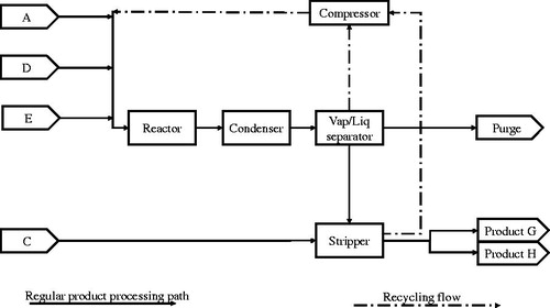
Reactants A, D and E flow into a reactor where the reaction takes place. The output from the reactor is fed to a condenser. Some non-condensable vapors join the liquid products, but the following vapor-liquid separator again splits the substances into separate flows. Vapor is partially recycled and partially purged together with the inert product and the byproduct. The stripper separates the remaining A, D and E reactants from the liquid and another reactant, C, is added to the product. The final products then exit the process and the remaining reactants are recycled.

The TE process has 12 manipulated variables (XMVs) and 41 measured variables (XMEAs). Tables in Downs and Vogel (1993) provide detailed information about all the process variables and the cost function that provides the process operating cost in $/h. The combination of three G/H mass ratios and four production rates of the final products define six different operating modes of the process. The user can also choose to activate 20 preset process disturbances (IDVs).

The TE process is open-loop unstable and it will rapidly leave the allowed process operations window and then shut down if it is run without engineering process control. Therefore, a control strategy is necessary for process stability. To avoid shutdowns and for securing plant safety, the control strategy should abide by five operating constraints related to the reactor pressure, level and temperature, the product separator level, and the stripper base level. Even with controllers working correctly, the TE process is sensitive and may shut down depending on the controller tuning and the set-points of the controlled variables.

Decentralized control strategy

The decentralized control strategy partitions the plant into sub-units and designs a controller for each one, with the intent of maximizing the production rate. Ricker (1996) identified nineteen feedback control loops to stabilize the process. Table 1 provides the control loops and the related controlled and manipulated variables. The original article by Ricker (1996) provides detailed information about the design phases of the decentralized control strategy.

Table 1. Controlled and manipulated variables in the 19 loops of the decentralized control strategy. The manipulated variables with codes such as F_p and r₇ come from the decentralized control strategy settings (Ricker 1996). XMV(i) and XMEAS(j) are numbered according to the original article by Downs and Vogel (1993).

Loop	Controlled variable	Code	Manipulated variable	Code
1	A feed rate (stream 1)	XMEAS(1)	A feed flow	XMV(3)
2	D feed rate (stream 2)	XMEAS(2)	D feed flow	XMV(1)
3	E feed rate (stream 3)	XMEAS(3)	E feed flow	XMV(2)
4	C feed rate (stream 4)	XMEAS(4)	A and C feed flow	XMV(4)
5	Purge rate (stream 9)	XMEAS(10)	Purge valve	XMV(6)
6	Separator liquid rate (stream 10)	XMEAS(14)	Separator pot liquid flow	XMV(7)
7	Stripper liquid rate (stream 11)	XMEAS(17)	Stripper liquid product flow	XMV(8)
8	Production rate (stream 11)	XMEAS(41)	Production index	Fp
9	Stripper liquid level	XMEAS(15)	Ratio in loop 7	r7
10	Separator liquid level	XMEAS(12)	Ratio in loop 6	r6
11	Reactor liquid level	XMEAS(8)	Set-point of loop 17	s.p. 17
12	Reactor pressure	XMEAS(7)	Ratio in loop 5	r5
13	Mol % G (stream 11)	XMEAS(40)	Adjustment of the molar feed rate of E	Eadj
14	Amount of A in reactor feed, yA(stream 6)	XMEAS(6)	Ratio in loop 1	r1
15	Amount of A+C in reactor feed, yAC(stream 6)	XMEAS(6)	Sum of loops 1 and 4 ratio	r1 + r4
16	Reactor temperature	XMEAS(9)	Reactor cooling water flow	XMV(10)
17	Separator temperature	XMEAS(11)	Condenser cooling water flow	XMV(11)
18	Maximum reactor pressure	XMEAS(7)	Production index	Fp
19	Reactor level override	XMEAS(8)	Compressor recycle valve	XMV(5)

The revised TE simulation model

Ricker (2005) devised the decentralized TE control strategy as a Simulink/Matlab® code. Bathelt et al. (2015b) recently developed a revised version of the simulation model. The revision is an update of Ricker's (2005) code that widens its usability by allowing for customization of the simulation by modifying a list of parameters in the process model function. Below we describe how to initialize the revised TE simulator and how to use the model function parameters to achieve intended simulator characteristics.

Initialization of the revised TE model

The files of the revised model are available as a Simulink/Matlab® code at the Tennessee Eastman Archive (Updated TE code by Bathelt et al. (2015b)). Figure 2 illustrates the workflow to initialize the simulator through a simulation test, using the BPMN standard (Chinosi and Trombetta 2012). The simulator requires three phases to be initialized: installation, test, and use. The installation mainly consists of downloading the files and setting them in the same computer directory. Then a simulation test can be launched to check if the installation has been successful. During the simulation test, four online plots display the reactor pressure, process operating cost, production flow, and product quality trend. When the simulation ends, the simulator provides datasets of XMVs and XMEAs as well as the related plots. The correct completion of the installation and test phases ensures that the simulator works properly and it is ready to be used. Initialization is then completed.

Figure 2. Main tasks required to initialize the simulator for operating Mode 1. Note that some symbols in the legend might be unused in this flowchart. Legend inspired by http://resources.bizagi.com/docs/BPMN_Quick_Reference_Guide_ENG.pdf

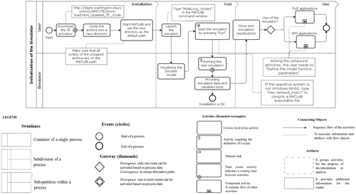
The simulator can be run in both operating Mode 1 and 3. Operating Mode 1, which we use in this article, seems to be the most commonly used in the literature. The model “MultiLoop_mode1” runs the process at Mode 1 when the set-points of the input variables not involved in control loops and of the controlled variables are set up according to the base case values given in Tables 2 and 3.

Table 2. Base case set-points of the input variables not involved in control loops for operating Mode 1.

Variable name	Code	Base case value (%)	Low limit (%)	High limit (%)
Compressor Recycle Valve	XMV(5)	22.210	0	100
Stripper Steam Valve	XMV(9)	47.446	0	100
Agitator Speed	XMV(12)	50.000	0	100

Table 3. Base case set-points of the controlled variables (available experimental factors) in the TE process for operating Mode 1.

Loop	Controlled variable	Base set-point
7	Stripper liquid rate (production)	22.949 m^3 h^−1
9	Stripper liquid level	50%
10	Separator liquid level	50%
11	Reactor liquid level	75%
12	Reactor pressure	2705 kPa
13	Mole % G	53.724 mol%
14	Amount of A in reactor feed (yA)	54.95%
15	Amount of A+C in reactor feed (yAC)	58.57%
16	Reactor temperature	120.40 ^oC

In Figure 2, “DoE applications” and “SPC applications” consist of different compound activities, expanded later, that the user must follow depending on which method is being applied. The definition of the model function parameters is one of these activities and can be done following the instructions below.

Using the model function parameters to customize the simulation

The model function “temexd_mod” contains the “TE code” and it is located in the “TE Plant” block of the Simulink model. A double-click on “temexd_mod” opens a dialog window. In the field “S-function parameters,” the user can define three model function parameters separated by commas. Square brackets are used for undefined parameters. The simulation can be customized to fit different needs by changing these parameters. Table 4 provides more details of the model function parameters.

Table 4. Description and settings of the parameter list for the process model function “temexd_mod” (Bathelt et al. 2015a). An example of settings for parameter 3 is given.

Parameter list of “temexd_mod”	Description		Setting
1	An array of the initial values of the 50 states of the model. The user can specify a vector of 50 states of the model to run the simulator in a specific operating mode		Empty: default values of process operating Mode 1 are used (Downs and Vogel 1993).
2	Initial value (seed) of the random generator		Every integer number greater than 0 is valid.
	Model structure flag
3	Bit	Description	Example	(11100010)2 = (226)10
	0	Additional measurements points	0	Integer value equivalent to the binary number activating/deactivating the bit of the model structure flag
	1	Monitoring outputs of the disturbances	1
	2	Monitoring outputs of the reaction and process	0
	3	Monitoring outputs of the component's concentration	0
	4	Deactivation of measurement noise	0
	5	Random generator uses different state variables for process disturbances and measurements noise	1
	6	Solver-independent calculations of the process disturbances	1
	7	Disturbances are scaled by the value of the activation flags	1
	15	Reset model structure to original structure of Ricker (2005)	0

Parameter 1 relates to the initial values of the model states. Since we wish to run the process in Mode 1, we hereafter assume that this parameter is set as empty unless otherwise specified. Therefore, the default “xInitial” array is used when we launch the simulator. Parameters 2 and 3 enable the customizations introduced in the revised TE code.

The possibility to change the seed of each simulation (parameter 2) creates the opportunity to avoid deterministic simulations, but only when the user activates process disturbances (IDVs) of the type random variation in the model, see Table 5. Parameter 3 allows for activating/deactivating the model flags listed in Table 4. Each model flag corresponds to a bit that can be switched using the binary notation. The value of parameter 3 corresponds to the decimal integer of the binary number obtained after setting the value of each bit. For example, the binary number (11100010)₂ is equivalent to the parameter value of (226)₁₀, which produces the exemplified model structure given in Table 4. Note that for the right conversion from a binary to a decimal number, the binary number must be written starting from the highest to the lowest bit position (from 15 to 0).

Table 5. The 28 process disturbances available (Downs and Vogel 1993, Bathelt et al. 2015a).

Variable Number	Process Variable	Type
IDV(1)	A/C feed ratio, B composition constant (stream 4)	Step
IDV(2)	B composition, A/C ratio constant (stream 4)	Step
IDV(3)	D feed temperature (stream 2)	Step
IDV(4)	Water inlet temperature for reactor cooling	Step
IDV(5)	Water inlet temperature for condenser cooling	Step
IDV(6)	A feed loss (stream 1)	Step
IDV(7)	C header pressure loss- reduced availability (stream 4)	Step
IDV(8)	A,B,C proportion in stream 4	Random variation
IDV(9)	D feed temperature (stream 2)	Random variation
IDV(10)	A and C feed temperature(stream 4)	Random variation
IDV(11)	Water inlet temperature for reactor cooling	Random variation
IDV(12)	Ater inlet temperatur for condenser cooling	Random variation
IDV(13)	Variation coefficients of reaction kinetics	Random variation
IDV(14)	Reactor cooling water valve	Sticking
IDV(15)	Condenser cooling water valve	Sticking
IDV(16)	Variation coefficient of the steam supply of the heat exchanger of the stripper	Random variation
IDV(17)	Variation coefficient of heat transfer in reactor	Random variation
IDV(18)	Variation coefficient of heat transfer in condenser	Random variation
IDV(19)	Unknown	Unknown
IDV(20)	Unknown	Random variation
IDV(21)	A feed temperature (stream 1)	Random variation
IDV(22)	E feed temperature (stream 3)	Random variation
IDV(23)	A feed flow (stream 1)	Random variation
IDV(24)	D feed flow (stream 2)	Random variation
IDV(25)	E feed flow (stream 3)	Random variation
IDV(26)	A and C feed flow (stream 4)	Random variation
IDV(27)	Reactor cooling water flow	Random variation
IDV(28)	Condenser cooling water flow	Random variation

As a rule of thumb, model flags 5 and 6 should be active during the simulation while the user can set the other model flags to adjust the model to the simulation needs. Further details of the model flag structure are given in Bathelt et al. (2015a).

Creating random simulations in the revised TE process simulator

The TE process is complex and in that sense mimics a real chemical process. While the high degree of complexity makes it useful as a testbed for methodological development, the same complexity imposes some limitations. As already stated, without customization, the TE simulator provides an output that does not differ much from a deterministic simulation where all measurement error is set to zero.

Figure 3 shows a schematic overview of the revised TE simulation model highlighting potential sources of random variation. Note that the TE process variables are only affected by white Gaussian noise mimicking typical measurement noise when random disturbances of type “random variation” are turned off. Thus, repeated simulations with the same setup will produce identical results, except for measurement error, which limit the model's value when running repeated simulations. Repeated simulations are for instance used when assessing the performance of an SPC method or when replicates of experimental runs are needed.

Figure 3. Schematic overview of the revised TE simulation model with a focus on potential sources of random variation.

To overcome this limitation, we suggest running the simulator with added measurement noise and one or more of the random disturbances (IDVs) listed in Table 5 activated. Indeed, the possibility to scale random variation disturbances allows the user to add variability without overly distorting the results. The possibility to change the seed is also important for our conclusion that the revised TE model is suitable for methodological tests of SPC and DoE methods.

It should be noted that the choice of the scale factor(s) to adjust the random variation depends on the random disturbance(s) introduced in the simulation model and the aim of the simulation study. The random disturbances vary in both magnitude and dynamics and hence impact the process differently. Therefore, we leave the choice of disturbances and the scale factor(s) to the user but explain the ideas behind our choices in our examples.

The TE process simulator in the SPC context

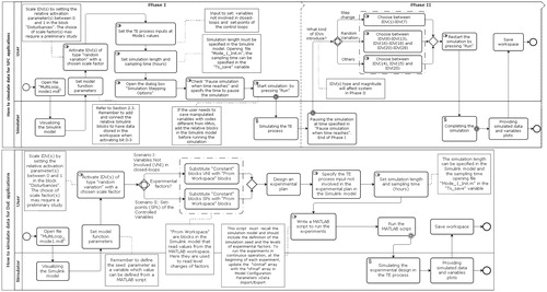
SPC applications require historical in-control data (Phase I dataset) and an online collection of data to perform Phase II analysis. Samples from Phase I and Phase II are typically collected in one shot in the TE process simulator. Using the BPMN standard, the upper half of Figure 4 presents the tasks required to simulate Phase I and Phase II data. Table 5 lists possible process disturbances (IDVs) that can be used as faults in Phase II. Note that the revised TE model adds eight “random variation” disturbances to the simulator, IDV(21)-IDV(28). A valuable characteristic of the revised simulator for SPC applications is the possibility to scale all process disturbances by setting their disturbance activation parameter values between 0 and 1.

Figure 4. Overview of tasks required to simulate data for SPC (upper) and DoE (bottom) applications. Symbols are explained in Figure 2.

Before we highlight three important SPC challenges that frequently occur in continuous processes and that the TE process simulator can emulate.

Multivariate data

The 53 variables available in the TE process (12 XMVs and 41 XMEAs), some of which are highly cross-correlated, allow for studies of multivariate monitoring methods. The TE process has been used extensively within the chemometrics literature to test monitoring applications and fault detection/isolation methods based on latent structures techniques such as principal component analysis (PCA) and partial least squares (PLS). The simulator does not produce missing data, but the analyst may remove data manually if needed.

Autocorrelated data

The user can choose the variables’ sampling rate in the TE process, but for most choices, the resulting data will be serially correlated (autocorrelated). Autocorrelation will require adjustment of the control limits of control charts since the theoretical limits will not be valid. This faulty estimation will affect in-control and out-of-control alarm rates (Bisgaard and Kulahci 2005, Kulahci and Bisgaard 2006), and this also extends to process capability analysis affecting both univariate and multivariate techniques.

Closed-Loop Operation

Closed-loop engineering process control is constantly working to adjust process outputs through manipulated variables, which represents an interesting SPC challenge. Control charts applied to controlled outputs could fail to detect a fault and might erroneously indicate an in-control situation. The traditional SPC paradigm to monitor the process output when engineering process control is in place requires proper adjustments and the TE process simulator provides a good testbed for this.

The TE process simulator in DoE context

The lower part of Figure 4 provides a guide on how to simulate data in using the TE process for testing DoE methods for continuous processes operating under closed-loop control. Note that one of the early tasks is to activate one or more process disturbances of type “random variation,” see Table 5, to overcome the deterministic nature of the simulator. Two experimental scenarios can, for example, be simulated using the TE process simulator (Capaci et al. 2017). In the first scenario, the experimental factors can include the three manipulated variables not involved in control loops, XMV(5), XMV(9), and XMV(12), see also Table 2, while the responses can include both manipulated and controlled variables. In the second scenario, the experimenter can use the set-point values of the control variables as experimental factors and the operating cost function as a response. However, a cascaded procedure based on directives generated by the decentralized control strategy will make some set-points dependent. Therefore, the experimenter only has the subset of the nine set-points given in Table 3 available as experimental factors in the second scenario.

The TE process simulator allows the user to pause, analyze the experiment, and make new choices based on the results. Thus, sequential experimentation, a cornerstone in experimental studies, is possible to simulate. The experimenter can repeat the experimental runs and expand the experiment with an augmented design since the seeds for the random disturbances can be changed. Hence, TE process simulator can emulate potential experimentation strategies such as response surface methodology (Box and Wilson 1951) and evolutionary operation (Box 1957). Even though cost and time concerns are irrelevant when experiments are run in a simulator and the number of experimental factor levels and replicates are practically limitless compared to a real-life experiment, there are only a few potential experimental factors available. The simulator may aid studies on the robustness and the analysis of an experiment where the number of experimental runs is limited, such as unreplicated designs with a minimum number of runs.

Below we highlight three challenges for the analyst when applying DoE in the TE process. These challenges are also commonly found in full-scale experimentation in continuous processes:

The closed-loop environment

The TE process experimenter must select experimental factors and analyze process responses while taking into account the presence of feedback control systems (Capaci et al. 2017). The decentralized control of the TE process will mask relationships between process input and output (see also McGregor and Harris 1990), and feedback control loops will limit the possibility to vary all the process inputs freely. Furthermore, the experimenter must restrict potential experimental factor changes within constrained operating regions to avoid any process shutdowns. As in open-loop systems, the choice of the experimental factor levels becomes crucial to assure the closed-loop process stability. However, one cannot expect the experimenter, new to the TE process, to predict the process behavior due to experimental factor changes. Instead, we have found that a trial-and-error approach of sufficiently stable operating regions has given sufficient a-priori knowledge of potentially feasible operating regions (such an approach is, of course, unfeasible in the real process case as it potentially involves multiple process shutdowns.) Later, results of the experimentation can provide an improved posteriori knowledge of actual feasible operating regions. Therefore, DoE methods can be used for factor screening, factor characterization, or process improvement and optimization in these processes. Moreover, it is fair to assume that a subsequent re-tuning of the control parameters at different sub-regions within the whole tolerable experimental region might lead to a further improvement of the process and an expansion of the region of tolerable operating conditions.

Transition times between runs

The time required for different responses to reach a new steady state in the TE process will differ depending on the factors and the magnitude of the change. The characterization of transition times is crucial to minimize their effect on the experimental results as well as to allocate the time needed for the treatments to take full effect (Vanhatalo et al. 2010). Long transition times between steady-state conditions add to the costs of randomizing the runs in a real experiment. The literature suggests using split-plot designs to restrict factor changes in this situation. Moreover, it is common to avoid resetting the levels of factors between consecutive runs where the factors are to be held at the same level for time and cost concerns. However, maintaining the factor level settings between adjacent runs and disregarding resetting lead to a correlation between neighboring runs and to designs called randomized-not-reset (RNR) designs (Webb et al. 2004). These can also be studied in the TE process.

Time series data for factors and responses

The continuous nature, the dynamic behavior, and the transition times of the TE process make it necessary to view experimental factors and responses as time series. The analysis of the experiments from the TE process allows for considering the time series nature of factors and responses. The response time series need to be summarized in averages or standard deviations to fit in a standard analysis such as the analysis of variance (ANOVA). Transfer function-noise modeling may be used to model the dynamic relations between experimental factors and the response(s) (Lundkvist and Vanhatalo 2014).

Example 1: The TE process simulator and SPC

Note that the aim of the example provided here (and in Section 6) is not to describe the most complex scenario available nor is it to suggest the “best solution” to the illustrated challenges. The examples are provided to show how the TE process can act as a testbed for developing and testing methodological ideas. In the first example, we illustrate how closed-loop operation can affect the shift detection ability of control charts. In particular, this example demonstrates how control charts applied to the (controlled) output could fail to detect a fault and, therefore, might erroneously indicate an in-control situation. It should be noted that this issue has been already handled in other research articles, see, for example, Rato and Reis 2014, 2015, and here we make use of it for illustration purposes.

The example focuses on control loops 9–12 and 16 (Table 1). These loops regulate the process operating constraints needed to secure plant safety and to avoid unwanted shutdowns. Five process inputs (r₅, s.p.₁₇, XMV(10), r_6, and r₇), i.e., the manipulated variables, control the related TE process outputs (XMEAS 7–9, 12 and 15). We here refer to control loops 9–12 and 16, and their related variables as critical control loops, critical controlled variables (C-XMEAS) and critical manipulated variables (C-XMVs) respectively.

Selecting and scaling disturbances

After a preliminary study of the process disturbances of type random variation (Table 5) available in the TE process, we further analyzed the behavior of IDV(8) and IDV(13). IDV(8) varies the proportion of the chemical agents (A, B, C) in stream 4 of the process, mimicking a reasonably realistic situation, whereas IDV(13) adds random variation to the coefficients of reaction kinetics, propagating its impact through the whole process. We performed 4 sets of 20 simulations each with a scale factor of the disturbances equal to 0.25, 0.5, 0.75 and 1 to understand the impact of IDV(8) and IDV(13) on process behavior. Each simulation, run with a randomly selected seed, lasted 200 hours in the TE process and the outputs of the random disturbances were collected with a sampling interval of 12 minutes. We kept constant the set-points of the inputs not involved in control loops and of the controlled variables at the base case values of operating Mode 1 (Tables 2 and 3).

Based on the averages and standard deviations presented in Table 6, to achieve random variation in the TE process, we ran Phase I and Phase II data collection with both IDV(8) and IDV(13) active, with randomly selected scale factors between 0 and 0.25 and, 0 and 0.5 respectively.

Table 6. Averages and standard deviations of IDV(8) and IDV(13) based on 20 simulations. Step size of IDV(4) for different scale factor values.

Variable number	Process variable	Scale factor	Average	Step size	Standard deviation
IDV(4)	Cooling water inlet temperature of reactor	0.25n n = 0,1,…,4	35	+1.25n	-
					n = 1	n = 2	n = 3	n = 4
IDV(8)	Proportion of A in stream 4	0.25n	48.51		0.372	0.748	1.126	1.50
	Proportion of B in stream 4	0.25n	0.50		0.038	0.074	0.110	0.15
	Proportion of C in stream 4	0.25n	50.99		0.374	0.751	1.130	1.51
IDV(13)	Variation coefficient of reaction kinetics A + C + D → G	0.25n	1		0.03n
	Variation coefficient of reaction kinetics A + C + D → G		1

We then performed a preliminary simulation with the same simulator settings for the random disturbances to select the magnitude of the step size (fault) for Phase II. Table 6 shows the magnitude of the step size for the scale factor equal to 0.25, 0.5, 0.75 and, 1. We, therefore, introduced a step change in the cooling water inlet temperature of the reactor in Phase II, i.e., IDV(4), with a randomly selected scale factor between 0.25 and 0.5.

Data collection

The TE process was first run for 144 hours at normal operating conditions (Phase I), i.e., base case values for operating Mode 1. A step change in the cooling water inlet temperature of the reactor (IDV4) was then introduced in the process for 108 hours (Phase II). The randomly selected scale factors of disturbances IDV(4), IDV(8) and IDV(13) in this simulation were 0.32, 0.1 and 0.25 respectively. Values on C-XMEAS and C-XMVs were collected in sequence during continuous operation of the process with a sampling time of 12 minutes.

Multivariate process monitoring

For illustration purposes, consider a standard Hotelling T² multivariate control chart for individual observations for the five critical controlled variables of the TE process (C-XMEAS). The Phase I sample was produced by excluding the start-up phase of the process. The critical controlled variables exhibit a dynamic behavior for about 36 hours or 180 samples at the start of the simulation. After this “warm-up phase,” the TE process was deemed to have reached steady-state.

Samples of C-XMEAS collected during steady-state operation provide a more stable estimation of the sample covariance matrix, S, and thus of the T² values. We discarded the first 180 observations and used datasets of 540 samples both in Phase I and Phase II to build the Hotelling T² chart, see Figure 5. The standard sample covariance matrix was used to form the T² chart. The theoretical Phase I and Phase II upper control limits were based on the β and F distributions and on the assumption that observations are time-independent (Montgomery 2012). This assumption is unrealistic because of the observed positive autocorrelation in the critical controlled variables (and as a result also in the T² values), and consequently, the upper control limits should be adjusted, see Vanhatalo and Kulahci (2015). However, the point we want to make here will still be evident from the appearance of Figure 5 using the theoretical control limits and we here intentionally avoid a detailed discussion on adjusted control limits.

Figure 5. Hotelling T² chart based on individual observations for the C-XMEAS (top) C-XMVs (bottom). The vertical line divides Phase I and Phase II data.

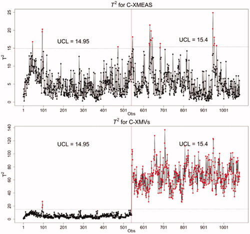
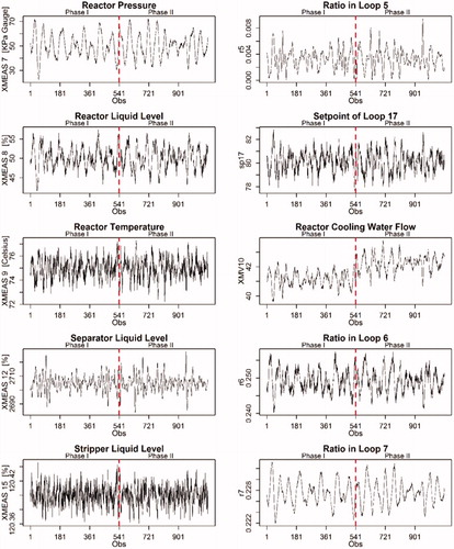
There are a few T² observations above the control limit in the Phase II sample based on C-XMEAS (top panel in Figure 5), but an analyst might as well conclude that there is little evidence to deem the process out-of-control. Moreover, a visual inspection of the C-XMEAS univariate plots in Figure 6 seems to support this conclusion, as the critical controlled variables appear to be insensitive to the step change in the cooling water inlet temperature of the reactor (IDV4). However, this conclusion is incorrect. Since the TE process is run in closed-loop operations, the analyst should know that the engineering process control seeks to displace most of the variability induced by the step change (fault) to some manipulated variable(s). In fact, the correct conclusion in this scenario is that the process is still working at the desired targets thanks to the feedback control loops. If the C-XMVs are studied, the analyst would probably deem the process to be out-of-control. That the process is disturbed becomes evident by studying the Hotelling T² chart based only on the five C-XMVs (bottom panel in Figure 5). While one may consider the process in control during Phase I, it is out-of-control in Phase II. Moreover, a visual inspection of the univariate C-XMVs plots in Figure 6 suggests that an increase in the flow of the reactor cooling water, XMV(10) compensates for the effect of the introduced fault in the inlet temperature. Such a control action could, of course, increase waste of water and/or energy while trying to maintain product properties on target.

Figure 6. Univariate time series plots for C-XMEAS (left column) and C-XMVs (right column) during both Phase I and II.

Closing remarks

The example above shows a possible application of how to use the TE process as a testbed for SPC methods. As the TE process is run in closed-loop operation, control actions may partly or entirely displace the impact of a disturbance from the controlled variables to manipulated variables. The traditional approach of applying a control chart on the (controlled) process output then needs to be supplemented with a control chart on the manipulated variables. The concurrent use of both of these control charts allows for [1] confirming the presence and effectiveness of the controller by analyzing the control chart for the controlled variables and [2] identifying potential assignable causes by analyzing the control chart for the manipulated variables.

Example 2: DoE in TE process simulator

This example illustrates a response surface methodology approach based on sequential experimentation using a subset of the set-points of the control loops in the TE process. The example starts with a two-level fractional factorial design, which is augmented to a central composite design, followed by confirmation runs in the simulator. The example describes how to use the TE process for experimentation. Hence, we conduct a simplified analysis of the experimental results applying ANOVA on the average values of the time series of the factors and the response of each experimental run, as suggested by Vanhatalo et al. (2013).

Closed-loop process performance may improve by exploring the relationships between the set-points of the controlled variables and an overall performance indicator such as production cost. Consider an experiment where we first want to identify reactor set-points that affect the operating cost and then aim to minimize this cost. Our experimental factors are in this case the five set-points of the controlled variables in loops 11, 12, 14, 15 and 16. The response is the process operating cost ($/h). Table 7 presents the set-points of the starting condition, the average operating cost (long-term value) given these set-points, and the chosen levels of the set-points in the two-level experimental design. Note that the choices of experimental factor levels were found using trial-and-error by changing the base case values, testing that these values yield a stable process. The input variables that were not involved in control loops were set at operating Mode 1 values (Table 2) in all simulations.

Table 7. Long-term average operating cost at the set-points of the starting condition. Low and high level of the set-points used as experimental factors.

Loop	Controlled variable	Set-points of the starting condition	Low level	High level
7	Stripper liquid rate (production)	22.949 m^3 h^−1	-	-
9	Stripper liquid level	50%	-	-
10	Separator liquid level	50%	-	-
11	Reactor liquid level	75%	70%	75%
12	Reactor pressure	2705 kPa	2600 kPa	2705 Kpa
13	Mole % G (product quality)	62 mol%	-	-
14	Amount of A in reactor feed (yA)	54.95%	55%	65%
15	Amount of A+C in reactor feed (yAC)	58.57%	50%	59%
16	Reactor temperature	120.40 ^oC	120 ^oC	127 ^oC
Long-term average operating cost		147.60 $/h

Selecting and scaling disturbances

Real processes are often disturbed by unknown sources. The random process variation in the simulator needs to be comparable to disturbances affecting a real process. We used the random disturbances IDV(8) and IDV(13) to add random disturbances to the process. The impact of IDV(8) on the operating costs of the process was studied using ten simulations with the starting set-points given in Table 7. The scale factor of IDV(8) was then increased in increments of 0.1 in each run. Each simulation, run with a random seed, lasted 200 hours (simulation time, not real time) and the operating cost was sampled every 12 minutes (simulation time). We repeated the procedure for IDV(13), increasing the scale factor in increments of 0.1 in each run. Visual inspection of the resulting cost time series led us to the conclusion that the scale factors for both IDV(8) and IDV(13) should be set between 0.1 and 0.4 to produce reasonable random variability.

The scale factors of IDV(8) and IDV(13) were set to 0.31 and 0.1 respectively throughout the simulations after drawing random numbers from a uniform distribution between 0.1 and 0.4. From another set of 20 simulations with these selected scale factors, the average (long-term) operating costs were 147.60 $/h with a standard deviation of 36.75 $/h. Visual inspection shows that the process operating cost exhibits a transition time of approximately 24 hours before reaching the steady state. Therefore, we removed observations of the cost function during the first 24 hours before calculating the average and standard deviation of the time series of the process operating cost.

Experimental design and analysis

Analyses reported in this section were all made using Design Expert® version 10.

Phase I: Screening

We chose a 2^5 − 1_V fully randomized fractional factorial design with four additional center runs to screen the five factors (reactor set-points) in Table 7. The experiment started by a “warm-up phase” where the TE process was run for 36 hours (180 samples) using the starting set-point settings in Table 7. After these 36 hours, the TE process was deemed to have reached steady-state. At steady-state, all runs were conducted in sequence according to their run order during continuous process operation. The simulation runs lasted 50 hours each (250 samples) and the simulation seed was randomly changed before each run. The operating cost was sampled every 12 minutes.

We calculated response averages for each run to analyze the response time series of the cost. We removed the observations of the transition time before calculating the run averages to avoid a biased estimation of the main effects and their interactions (Vanhatalo et al. 2013). The transition time during some runs was determined to be approximately 24 hours through visual inspection. Some settings thus affected process stability, which meant that the run averages were based on the run's last 26 hours (130 samples). Table 8 shows the run order during the experiment and the averages of the process operating cost for each run.

Table 8. Run order, standard order of the runs, and average operating cost after removing the transition time at the beginning of each run. The “c” in standard order marks the center points.

Block 1: 2^5 − 1V						Block 2: Augmented plan
Run order	Standard order	Operating Cost ($/h)	Run order	Standard order	Operating Cost ($/h)	Run order	Standard order	Operating Cost ($/h)
1	9	163.66	11	17c	128.83	21	27	147.82
2	14	162.79	12	19c	126.96	22	22	135.91
3	12	155.84	13	3	144.00	23	21	126.96
4	10	175.84	14	13	175.24	24	28	189.13
5	7	127.38	15	2	180.51	25	29	168.99
6	18c	131.29	16	1	140.62	26	26	136.39
7	20c	123.26	17	16	159.84	27	24	117.51
8	6	145.13	18	8	136.36	28	30	163.25
9	5	151.53	19	11	158.39	29	23	147.95
10	4	129.90	20	15	136.09	30	25	140.13

Table 9 presents an ANOVA table of active effects (at 5% significance level) based on the first 20 experimental runs of Table 8. Four main effects and two two-factor interactions have statistically significant effects on the operating cost. We also included the main effect of factor E in the model due to effect heredity. However, the significant curvature suggests that a higher order model may be needed.

Table 9. ANOVA and estimated effects based on the first 20 runs in Table 8. Third order and higher interactions are ignored.

Source	Sum of Squares	df	Mean Square	F Value	Prob > F	Estimated Standardized Effects ($/h)
Model	3941.46	7	563.07	29.65	< 0.0001
A: Reactor Liquid Level	151.89	1	151.89	8.00	0.0164	3.08
B: Reactor Pressure	1360.21	1	1360.21	71.64	< 0.0001	-9.22
C: Amount of A in the reactor feed (yA)	184.90	1	184.90	9.74	0.0097	-3.40
D: Amount of A+C in the reactor feed (yAC)	1093.39	1	1093.39	57.58	< 0.0001	8.27
E: Reactor Temperature	21.22	1	21.22	1.12	0.3131	-1.15
CE	225.63	1	225.63	11.88	0.0055	3.76
DE	904.21	1	904.21	47.62	< 0.0001	7.52
Curvature	2017.86	1	2017.86	106.27	< 0.0001	3.08
Residual	208.87	11	18.99
Lack of Fit	174.46	8	21.81	1.90	0.3234
Pure Error	34.41	3	11.47
Cor Total	6168.18	19
				R^2		63.90%
				Adjusted R^2		42.84%
				R^2 prediction		34.71%

Phase 2: Second-order model

Augmenting the resolution V fractional factorial design with ten additional axial points run in a new block produced a central composite design, allowing for estimation of a second-order model. We simulated the second block of experimental runs in sequence as a continuation of the first 20 runs and used the same procedure to calculate run averages as in the first block. We did not impose any blocking effect in the simulations. The analysis of the 30-run augmented design gives the second-order model shown in the ANOVA table (Table 10). The residual analysis indicated that the 15^th run (standard order #2) could be an outlier. However, since we did not find a reasonable explanation for this outlier, we chose to include it in the model despite a slight decrease in the R², R² adjusted, and R² predicted statistics. Table 10 thus presents the ANOVA table of the augmented design in Table 8 (5% significance level). The non-significant lack of fit and the high values of the R² statistics indicate that the model fits the data well and has good predictive ability.

Table 10. ANOVA and estimated effects for the augmented design using observations in both blocks. The model includes only those terms significant on a 5% significance level. Third order and higher interactions are ignored.

Source	Sum of Squares	df	Mean Square	F Value	Prob > F	Estimated Standardized Effects ($/h)
Block	0.49	1	0.49
Model	9896.57	10	989.66	51.10	< 0.0001
A: Reactor Liquid Level	188.15	1	188.15	9.72	0.0060	2.80
B: Reactor Pressure	1809.73	1	1809.73	93.45	< 0.0001	-8.68
C: Amount of A in the reactor feed (yA)	159.56	1	159.56	8.24	0.0102	-2.58
D: Amount of A+C in the reactor feed (yAC)	1924.18	1	1924.18	99.36	< 0.0001	8.95
E: Reactor Temperature	37.30	1	37.30	1.93	0.1821	-1.25
CE	225.63	1	225.63	11.65	0.0031	3.76
DE	904.21	1	904.21	46.69	< 0.0001	7.52
C^2	160.68	1	160.68	8.30	0.0100	2.40
D^2	2772.06	1	2772.06	143.14	< 0.0001	9.95
E^2	2453.31	1	2453.31	126.68	< 0.0001	9.36
Residual	348.58	18	19.37
Lack of Fit	314.17	15	20.94
Pure Error	34.41	3	11.47
Cor Total	10245.64	29
				R^2		96.60%
				Adjusted R^2		94.71%
				R^2 prediction		89.49%

We then minimized the operating cost within the experimental design region spanned by the low and high levels of the factors in Table 7 based on the model in Table 10. The numerical optimization tool in the Design Expert® was used to search the design space, and Table 11 presents the settings of the reactor set-points that result in the lowest predicted cost.

Table 11. The suggested setting of the reactor set-points to obtain lowest operating cost.

Loop	Controlled variable	Suggested set-points setting
7	Stripper liquid rate (production)	Not in model (refer to Table 7)
9	Stripper liquid level	Not in model (refer to Table 7)
10	Separator liquid level	Not in model (refer to Table 7)
11	Reactor liquid level	70.37%
12	Reactor pressure	2701.30 kPa
13	Mole % G (product quality)	Not in model (refer to Table 7)
14	Amount of A in reactor feed (yA)	63.67%
15	Amount of A+C in reactor feed (yAC)	52.25%
16	Reactor temperature	124.25 ^oC
Estimated process operating cost		117.07 $/h

Phase 3: Confirmation runs

Three additional confirmation runs were simulated in the TE process using the suggested set-points (Table 11). The average cost of these runs was 117.16 $/h. An average operating cost of 117.16 $/h represents a reduction of 30.44 $/h compared to the operating cost when starting set-point values are used, a reduction that we assume most production engineers would deem considerable.

Closing remarks

The sequential experimentation example illustrates how DoE methodologies can be explored in processes where engineering process control is present using the TE process simulator as a testbed. The example shows how a continuous process operating in closed-loop can be improved by shifting the set-points of the controlled variables. Experimental plans can help to explore the relationship between set-points and overall process performance indicators such as process cost or product quality. Note that the change in operating conditions invoked by the recommended change of the set-points may require re-tuning of the controllers in the system. We have not done that. That is, we assume that the control configuration and settings can still maintain the stability of the system in the new operating condition based on the new set-points. In our approach, we use DoE as a systematic solution to reduce the cost of the TE process based on an existing control system without redesigning it. As such, it resembles ideas in the so-called retrofit self-optimizing control approach from the engineering control domain described by Ye et al. (2017).

Conclusions and discussion

The TE process simulator is one of the more complex simulators available that offers possibilities to simulate a nonlinear, dynamic process and operates in closed-loop useful for both methodological research and teaching. In this article, we provide guidelines for using the revised TE process simulator, run with a decentralized control strategy, as a testbed for new SPC and DoE methods. In our experience, understanding the details of the TE process simulator and getting it to run may be challenging for novice users. The main contribution of this article is the flowcharts coupled with recommended settings of the TE process that will help a novice user of the simulator to get started. Another contribution is the suggested approach of how to induce random variation in the simulator. The possibility of introducing random variability in the simulator improves the usability of the TE process simulator in SPC and DoE contexts. This way, independent simulations can now be produced for SPC applications and independent replicates can be run in an experimental application.

In the two examples provided, we illustrate some of the challenges that an analyst normally faces when applying SPC and DoE in continuous processes operating under closed-loop control. We would like to reiterate that the illustrated examples are only examples of applications for which the TE process simulator can be used. We believe that the revised TE process simulator offers ample opportunities for studying other and more complicated scenarios that will mimic real-life applications.

SPC methods do not jeopardize the production or the product quality since these methods use observational data and require human intervention if out-of-control situations are indicated. For instance, in a real scenario, the process engineer may deem that the out-of-control situation is too marginal to stop the process for corrective actions but keep the disturbance in mind the next time the process is overhauled. However, when developing and testing SPC methods, the revised TE process simulator can quickly provide datasets with the desired characteristics as, for example, sample size, sampling time, or occurrence of a specific fault.

Unlike SPC methods, developing of DoE methods requires data from a process that was deliberately disturbed and getting access to such data could mean loss of product quality or risking the plant integrity. Consequently, the method developer will have trouble getting production managers to accommodate requests for disturbing the processes, just for the sake of developing new methods. Experimental campaigns in continuous processes tend to be lengthy and expensive. Therefore, simulators are particularly useful for developing DoE methods in such environments.

As a suggestion for further research, the possibility to develop other statistically based methods such as times series modelling or predictive analytics to be useful for a continuous process environment using the revised TE process in other applications on a wide variety of topics should of course be possible.

About the authors

Francesca Capaci is a doctoral candidate in Quality Technology at Luleå University of Technology (LTU) in Sweden. She has a Master's degree in Industrial and Management Engineering from the University of Palermo, Italy. Her research is focused on experimental design and statistical process control for continuous processes. She is a member of the European Network for Business and Industrial Statistics (ENBIS).

Erik Vanhatalo is associate professor of Quality Technology at LTU. He holds an MSc degree in Industrial and Management Engineering and Ph.D. in Quality Technology from LTU. His research is mainly focused on the use of statistical process control, experimental design, time series analysis, and multivariate statistical methods, especially in the process industry. He is a member ENBIS.

Murat Kulahci is a professor of Quality Technology at LTU and Associate Professor in theDepartment of Applied Mathematics and Computer Science, at the Technical University of Denmark. His research focuses on the design of physical and computer experiments, statistical process control, time series analysis and forecasting, and financial engineering. He has presented his work in international conferences, and published over 70 articles in archival journals. He is the co-author of two books on time series analysis and forecasting.

Bjarne Bergquist is Professor and Chair of Quality Technology LTU. His current research interests are focused on the use of statistically based methods and tools for improvements, particularly in the continuous process industries, as well as on statistically based railway maintenance. He has a background in Materials Science but lately has mainly published in the field of operations management, quality technology, and quality improvements.

Acknowledgements

We gratefully acknowledge the constructive suggestions made by the two reviewers of the paper.

Additional information

Funding

The authors gratefully acknowledge the financial support from the Swedish Research Council under grant number 340-2013-5108.

References

- Bathelt, A., Ricker, N.L., and Jelali, M. (2015a). Revision of the Tennessee Eastman Process Model. IFAC-PapersOnLine, 48(8):309–314.
- Bathelt, A., Ricker, N.L., and Jelali, M. (2015b). Tennessee Eastman Challenge Archive. http://depts.washington.edu/control/LARRY/TE/down-load.html#Updated_TE_Code. (accessed 2017 May).
- Bisgaard, S., and Kulahci, M. (2005). Quality Quandaries: The Effect of Autocorrelation on Statistical Process Control Procedures. Quality Engineering, 17(3):481–489.
- Box, G.E.P. (1957). Evolutionary Operation: A Method for Increasing Industrial Productivity. Journal of the Royal Statistical Society. Series C (Applied Statistics), 6(2):81–101.
- Box, G.E.P., and Wilson, K.B. (1951). On the Experimental Attainment of Optimum Conditions. Journal of the Royal Statistical Society, Series B (Methodological) 13(1):1–45.
- Capaci, F., Bergquist, B., Kulahci, M., and Vanhatalo, E. (2017). Exploring the use of design of experiments in industrial processes operating under closed-loop control. Quality and Reliability Engineering International. 33:1601–1614. doi:10.1002/qre.2128.
- Chinosi, M., and Trombetta, A. (2012). BPMN: An Introduction to the Standard. Computer Standards & Interfaces, 34(1):124–134.
- Dennis, D., and Meredith, J. (2000). An Empirical Analysis of Process Industry Transformation Systems. Management Science, 46 (8):1058–1099.
- Downs, J.J., and Vogel, E.F. (1993). A Plant Wide Industrial Process Control Problem. Computers & Chemical Engineering, 17(3):245–255.
- Ferrer, A. (2014). Latent Structures-Based Multivariate Statistical Process Control: A Paradigm Shift. Quality Engineering, 26(1):72–91.
- Ge, Z., Song, Z., and Gao, F. (2013). Review of Recent Research on Data-Based Process Monitoring. Industrial & Engineering Chemistry Research, 52(10):3543–3562.
- Hsu, C., Chen, M., and Chen, L. (2010). A Novel Process Monitoring Approach with Dynamic Independent Component Analysis. Control Engineering Practice, 18(3):242–253.
- Kruger, U., Zhou, Y., and Irwin, G.W. (2004). Improved Principal Component Monitoring of Large-Scale Processes. Journal of Process Control, 14(8):879–888.
- Ku, W., Storer, R.H., and Georgakis, C. (1995). Disturbance Detection and Isolation by Dynamic Principal Component Analysis. Chemometrics and Intelligent Laboratory Systems, 30(1):179–196.
- Kulahci, M., and S. Bisgaard. (2006). Challenges in Multivariate Control Charts with Autocorrelated Data. Proceedings to the 12th ISSAT International Conference on Reliability and Quality in Design, Chicago, IL.
- Lee, G., Han, C., and Yoon, E.S. (2004). Multiple-Fault Diagnosis of the Tennessee Eastman Process Based on System Decomposition and Dynamic PLS. Industrial & Engineering Chemistry Research, 43(25):8037–8048.
- Liu, K., Fei, Z., Yue, B., Liang, J., and Lin, H. (2015). Adaptive Sparse Principal Component Analysis for Enhanced Process Monitoring and Fault Isolation. Chemometrics and Intelligent Laboratory Systems, 146:426–436.
- Lundkvist, P., and Vanhatalo, E. (2014). Identifying Process Dynamics through a Two-Level Factorial Experiment. Quality Engineering, 26(2):154–167.
- Lyman, P.R., and Georgakis, C. (1995). Plant-Wide Control of the Tennessee Eastman Problem. Computers & Chemical Engineering, 19(3): 321–331.
- McGregor, J., and Harris, T.J. (1990). Exponentially Moving Average Control Schemes: Properties and Enhancements – Discussion. Technometrics, 32(1): 23–26.
- Montgomery, D. (2012). Statistical process control: A modern introduction. 7th ed., Hoboken (NJ): Wiley.
- Rato, T.J., and Reis, M.S. (2013). Fault Detection in the Tennessee Eastman Benchmark Process using Dynamic Principal Components Analysis Based on Decorrelated Residuals (DPCA-DR). Chemometrics and Intelligent Laboratory Systems, 125:101–108.
- Rato, T.J., and Reis, M.S. (2014). Sensitivity enhancing transformations for monitoring the process correlation structure. Journal of Process Control, 24:905–915.
- Rato, T.J., and Reis, M.S. (2015). On-line process monitoring using local measures of association: Part I – Detection performance. Chemometrics and Intelligent Laboratory Systems, 142: 255–264.
- Reis, M., and Kenett, R.S. (2017). A Structured Overview on the use of Computational Simulators for Teaching Statistical Methods. Quality Engineering, 29(4):730–744.
- Ricker, L.N. (1996). Decentralized Control of the Tennessee Eastman Challenge Process. Journal of Process Control, 6(4):205–221.
- Ricker, L.N. (2005). Tennessee Eastman Challenge Archive. http://depts.washington.edu/control/LARRY/TE/download.html#Decentralized_control (accessed 2017 May).
- Ricker, L.N., and Lee, J.H. (1995). Non-Linear Model Predictive Control of the Tennessee Eastman Challenge Process. Computers & Chemical Engineering, 19(9): 961–981.
- Vanhatalo, E., Bergquist, B., and Vännman, K. (2013). Towards Improved Analysis Methods for Two-Level Factorial Experiment with Time Series Responses. Quality and Reliability Engineering International, 29(5):725–741.
- Vanhatalo, E., Kvarnström, B., Bergquist, B., and Vännman, K. (2010). A Method to Determine Transition Time for Experiments in Dynamic Processes. Quality Engineering, 23(1):30–45.
- Vanhatalo, E., and Bergquist, B. (2007). Special Considerations when Planning Experiments in a Continuous Process. Quality Engineering, 19(3):155–169.
- Vanhatalo, E., Kulahci, M., and Bergquist, B. (2017). On the Structure of Dynamic Principal Component Analysis used in Statistical Process Monitoring. Chemometrics and Intelligent Laboratory Systems, 167:1–11.
- Vanhatalo, E. and Kulahci, M. (2015). The Effect of Autocorrelation on the Hotelling T2 Control Chart. Quality and Reliability Engineering International, 31(8):1779–1796.
- Vining, G., Kulahci, M., and Pedersen, S. (2015). Recent Advances and Future Directions for Quality Engineering. Quality and Reliability Engineering International, 32(3):11–21.
- Webb, D.F., Lucas, J.M., and Borkowski, J.J. (2004). Factorial Experiments when Factor Levels are Not Necessarily Reset. Journal of Quality Technology, 36(1):1–11.
- Ye, L., Cao, Y., Yuan, X., and Song, Z. (2016). Retrofit self-optimizing control of Tennessee Eastman Process. Industrial Electronics IEEE Transactions 64:4662–4670. ISSN 0278-0046.