Exploratory text data analysis for quality hypothesis generation

Abstract

Freestyle text data such as surveys, complaint transcripts, customer ratings, or maintenance squawks can provide critical information for quality engineering. Exploratory text data analysis (ETDA) is proposed here as a special case of exploratory data analysis (EDA) for quality improvement problems with freestyle text data. The EDTA method seeks to extract useful information from the text data to identify hypotheses for additional exploration relating to key inputs or outputs. The proposed four steps of ETDA are: (1) preprocessing of text data, (2) text data analysis and display, (3) salient feature identification, and (4) salient feature interpretation. Five examples illustrate the methods.

Keywords:

• cyber security
• exploratory data analysis
• graphical data analysis
• pattern discovery
• quality improvement
• text analytics
• twitter analysis

Introduction

In this article, we propose exploratory text data analysis (ETDA) as a technique for use in the analysis of text-based data sets to generate hypotheses relating to system improvement. Quality engineers often have text data available on multiple subjects. These could be in the form of customer surveys, complaints, line transcripts, maintenance squawks, or warranty reports. Yet, they often lack the techniques to use these data effectively for quality improvement purposes.

Tukey (1977) proposed exploratory data analysis (EDA) as a general method for generating hypotheses using visualizations for statistical problems. De Mast and Trip (2007) proposed a prescriptive framework for applying EDA in the context of quality improvement projects. Here, we focus on EDA in the context of both quality improvement and text data. Therefore, ETDA is intended to be a special case of EDA and the associated quality framework of De Mast and Trip (2007). Beyond providing a set of techniques or data visualization methods, ETDA like EDA seeks to provide a set of principles and methods to guide the performance of data analysis (Tukey 1977).

As noted by Tukey (1977) and others, EDA contrasts with confirmatory data analysis (CDA). EDA seeks to generate hypotheses while CDA has the goal of testing existing hypotheses. For instance, in a regression/hypothesis testing problem, EDA might be conducted as a first step to identify possible regressors to include in a model using scatter or XY plots. The shot size in injection molding, for example, might be hypothesized to affect the fraction of nonconforming units. Once the model form is selected, then CDA proceeds to calculation of the p-values and interpretation of their implications for proving hypotheses. Then, proof might be generated that shot size does indeed affect the fraction of nonconforming units.

Another type of analysis called descriptive data analysis (DDA) is potentially used as part of both EDA and CDA (De Mast and Trip 2007). DDA is concerned with the summary of data, for example, statistics such as the sample mean and sample standard deviation. DDA also suppresses the uninformative part of the set to highlight its important features. In large-scale problems dealing with big data arrays, measurements such as means and standard deviations, visualizations in tables and graphs, or other descriptive statistics reduce the complexity of the data sets (Good 1983). DDA helps inquirers to prune unimportant data and focus on the salient features. In the context of our proposed ETDA framework, preprocessing of data may be viewed as DDA. Therefore, like EDA, ETDA is intended to be an extension of DDA.

As noted previously, ETDA is proposed to be a special case of EDA that analyzes plain text datasets to derive high-quality information in quality improvement topics. Allen and Xiong (2012) and Sui (2017) provide examples of the application of ETDA techniques in exploring Toyota Camry user reviews. Allen et al. (2016) leverage ETDA for hypothesis generation for call center improvement factors. Here, we seek to provide a prescriptive framework for ETDA for all quality improvement projects using real-life applications of ETDA from case studies like those used by De Mast and Trip (2007). These cases are selected to represent a variety of areas relevant to quality practitioners including automotive engineering, calling centers, and information technology. Even though the nature of text mining is associated with low signal-to-noise ratios, our framework can identify suggestive patterns in unstructured data.

In the following section, a motivating example is described which relates to consumer reports on the Toyota Camry. Next, we propose the ETDA framework and describes its relationship to the framework from De Mast and Trip (2007). Subsequent sections elaborate on the steps of the ETDA: identifying the problems and associated text data; preprocessing of the text data; text data analysis and display options; text data salient feature identification; and lastly salient identification interpretation. Four additional examples further illustrate the principles and methods. Finally, we offer remarks relating to the discussion of the issues that a practitioner might encounter while employing ETDA.

Example 1: Quality improvement for Toyota Camry

In the first example, the Toyota Camry consumer report dataset from Allen and Xiong (2012) is used. This dataset contains 1,067 records of user reports for the automobile model between the years 2000 to 2010. Additional details about the analysis method and “topic models” are shown in a later section. The data including customer complaint or survey results were available in many industries and were provided by Consumer Reports.

The records include fields of summary, pros, cons, comments, and driving experience. Here, only cons texts are analyzed to generate quality hypotheses. Natural language processing (NLP) and latent Dirichlet allocation (LDA) are applied using 10 topics. NLP and LDA are discussed in more detail in the next section and the Appendix. The resulting Pareto chart is given in Figure 1. In the chart, the clusters or topics are represented by the top words ranked using estimated posterior probability. The charted quantities are the estimated posterior cluster proportions following Allen and Xiong (2012).

Figure 1. Topic proportion for cons in Toyota Camry Consumer Report.

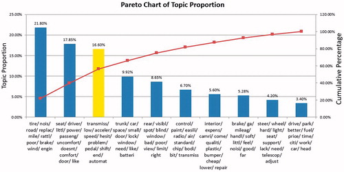
The first topic can be interpreted to mean that consumers are complaining about road noise or wind noise because of tire problems. This topic accounts for 21.80% of con words among the 10 topics. The second most frequent topic is about uncomfortable seating, accounting for 17.85%. This is consistent with the 2010 Camry recalls for seat heater/cooler problems caused by damage to electrical wiring in the seat heater when the seat cushion is compressed. The third most frequent topic (yellow column) verifies the well-known uncontrolled acceleration problem which embarrassed the Toyota Corporation during the 2009–2011 period.

The implications for quality improvement projects are clear. The data and charts serve to clarify that priority should be given to addressing the widely publicized unintended acceleration problem over tire noise and uncomfortable seats. Such analysis can not only help in putting problems into better perspective but also generate hypotheses for further investigation. Even complete remediation of the unintended acceleration would reduce only approximately 17% of the claims, although this was a catastrophic symbolic quality problem for Toyota.

The principles and framework of ETDA

In this section, we review the purposes of EDA from De Mast and Trip (2007) and describe the special context of text modeling and ETDA. Also, we clarify our extension of their framework. As noted by those authors, EDA’s main purposes are “to generate hypotheses”, “to generate clues”, “to discover influence factors”, and “to build understanding of the nature of the problem”. Like the EDA framework, the ETDA framework also seeks to reveal the potential relationships between key process output variables (KPOVs) in six sigma terminology or Y’s and the associated key process input variables (KPIVs) or X’s. Thus, the first principle formalizes the purpose:

A. The purpose of ETDA is to leverage text documents to help in the identification of dependent variables, Ys, and independent variables, Xs, that may prove to be of interest for understating or solving the problem under study.

De Mast and Trip (2007) draw a distinction between situations in which there is a relatively easy way to identify the key output variables (KOVs, Ys) and other situations. When it is easier to differentiate (situation #1), the total negative instances, for example, defects, are the sum of available categories of instances: (1) $$Y=Y_1+Y_2+Y_3+\cdots \mathrm{ }$$(1)

In these situations, EDA (and ETDA) should be able to identify the leading terms and associate hypotheses for clear follow-up activities. The first example in Figure 1 shows how ETDA identifies dependent variables (Ys) for further study using NLP and a popular clustering method called LDA (Blei, Ng, and Jordan 2003). Additional details about NLP and LDA are described in the next section. The important new element here is that word counts are associated with the quality issues rather than simple counts of nonconformities or other numerical process information.

In the second type of situation classified by De Mast and Trip (2007), the data are more limited. The practitioner can only identify that there is another lower level of attribution and analysis needed. Then, the sum of negative events is written: (2) $$Y=E_1+E_2+E_3+\cdots$$(2) where $E_i=f(X_{j1},X_{j2},\mathrm{ }{X}_{j3},\dots )$. The investigators could acquire clues about causal factors ($E_i$) by analyzing the text documents with respect to independent variables (Xs). A case study of how ETDA helps to identify clues for further investigation about independent variables (Xs) is described in Example 2.

De Mast and Trip (2007) proposed a three-step process for quality improvement-related EDA. Because of the complexities of text modeling, in ETDA the first step of their process is divided into two parts creating four steps:

1. Text data preprocessing.

2. Text data analysis and display.

3. Salient feature identification.

4. Salient feature interpretation.

The next sections describe additional principles elaborating on those in De Mast and Trip (2007) for these steps. The key aspects of text include the ability of the text data itself to directly provide causal insights in a way that ordinary data cannot.

While NLP is an entire field of inquiry with many possible complications, the general emphases of Tukey and EDA are transparency and simplicity (Tukey 1977). Therefore, the second ETDA (new) principle is as follows:

B1. NLP methods for ETDA should be simple with stop words that can be adjusted and standard stemming. Then, the users should perceive NLP as transparent and understandable.

In our examples, results are primarily based on simple word counts on different topics or clusters. Simple weightings of words associated with sentiment scores are also considered. Also, in general, NLP methods create word or document cluster “tags” and numerical values to permit further data exploration steps. This leads to the principle:

B2. Apply clustering methods to tag documents with numbers relating to cluster membership. These tags can be either manually or automatically generated and are useful for plotting and hypothesis generation.

Among the most widely cited and used methods for unstructured text clustering and automatic tag generation is LDA (Blei et al. 2003). LDA is described in more detail in the Appendix. LDA involves fitting a distribution to the words with probabilities often through Bayesian estimation of the chances that a random word is in a cluster (or “topic”) and that it will assume a specific selection from the dictionary, that is, the topic definition posterior mean probability estimates.

Both assigning words and document proportions to topics and defining topics through word probability estimates permit the study of quality issues at a higher granularity than the cluster level.

B3. Apply a simple and relatively transparent sentiment score analysis to transform the text to values (positive, zero, or negative numbers for further analysis).

There are many methods for assigning values to individual words, sentences, or documents relating to their positive or negative value (Liu 2012; Pang and Lee 2008; Turney 2002).

Text data preprocessing

Methods to permit word tabulations and sentiment analyses generally require NLP methods (Feldman and Sanger 2007). There are variants, of course. Yet, commonly irrelevant or “stop” words are first removed such as “of” and “a” which often offer limited contributions to meaning. Sometimes custom words with little meaning are manually added to stop word lists. Then, words are “stemmed” so that “qualities” and “quality” might become “quality” and, potentially, synonyms are replaced. Finally, the stemmed words are replaced by numbers for clustering or other analysis activities.

After the stop words are removed and the words are stemmed, a list of distinct words is called a “dictionary” for each set of documents. A simple approach used here to address multiple fields in a database is to append field titles to these stemmed nonstop words. Porter (1980) proposed an algorithm to handle words that have different forms for grammatical reasons as well as derivationally related words with similar meanings. Combining all these steps the methods used in the example are:

• Step 1. Split the document into words.

• Step 2. Remove the punctuation or symbols and (optionally) make all words lower case.

• Step 3. Remove the stopping words.

• Step 4. Stem the words with the Porter Stemming Algorithm.

• Step 5. Append the field titles in parentheses to each word (if appropriate).

Once the dictionary is available and the words are pre-processed, clustering and assignments of weights or “semantic” analysis are generally the primary techniques for additional processing.

Of primary interest in LDA is the probabilities defining the clusters or topics (“topic probabilities”) and the probabilities relating to the changes that words in specific documents relate to the topics (“document-topic” probabilities). The estimated mean values for these defining probabilities provide inputs to further analyses.

The direct Bayesian approach to estimate these mean posterior probabilities defining the clusters is called “collapsed Gibbs” sampling (Griffiths and Steyvers 2004; Teh et al. 2007). Allen et al. (2017) and Parker et al. (2017) created an approximate but relatively computationally efficient method for estimating the topic probabilities and the document-topic matrices based on k-means clustering. In this method, the clusters are used as topics by calculating the Euclidean distance from each quantified document to the estimated cluster centers and using the inverse of distance as the probabilities of the stemmed words falling in each topic (Sui and Allen 2016; Parker et al. 2016).

Some clusters might be associated with problems or customer complaints of specific nature, as we illustrate in Figure 1. Yet, in general, words in topic models do not have clear positive or negative interpretations. In many situations, methods that explicitly place values on words in the dictionary can facilitate additional insights.

In some cases, words could be related to emotional states such as “angry”, “anxious”, “happy”, “sad”, or “neutral”. In other cases, the “sentiments” could even be customized for quality professionals to tally a specified list of terms indicating likely quality defects. With arbitrariness, words can be rated individually with scores about their strengths. Here, to reduce the arbitrariness and for simplicity, words are generically rated as positive or negative. The sum of the positive words in a document is denoted by P and the sum of the negative words by N. The sentiment score (S) used in our examples is (3) $$S=\ln \left(0.5+P\right)-\ln \left(0.5+N\right).$$(3)

In general, our objectives for clustering and for sentiment scoring are to produce quantitative data to facilitate hypothesis generation. In the next section, we describe how the derived outputs can be used to create visualizations to aid in quality improvements.

Text data analysis and display

After preparing text-creating numbers relating to cluster identities and membership or sentiment score, one can follow steps 2–4 which derive from methods of De Mast and Trip (2007). Then, graphical presentations in ETDA can aid in highlighting and presenting findings to analysts (Good 1983; Hoaglin et al. 1983; Bisgaard 1996). Therefore, after preprocessing, the next step is to display text data in a straightforward way that exploits the power of pattern recognition.

C. Process and display the quantitative text data to reveal distributions and potential hypotheses for ways to improve system quality.

As for non-text EDA, graphical presentations can reveal what the inquirer did not expect beforehand (Bisgaard 1996). For EDTA, revealing patterns can relate to counts of words on specific topics (clusters) or differences across topics. At this phase, the primary visualization tools include Pareto or sorted bar charting methods, running charts, and so on to view different topics, contents, and quantitative text data. Note that, in Figure 1, the topic proportions are captured through Pareto charts. The inquirer could examine the topics from the largest probability to the least and, therefore, illuminate potential causes of defects.

C1 (Stratified Data). Process and display the quantitative text data so as to reveal distribution across and within strata.

Quality ratings can provide ordered strata. ETDA can help the inquirer to narrow down the searching range for the defects by focusing only on the low ratings into which defects mostly fall. Hence, practitioners can display cluster information at different strata levels to generate hypothesis for design inputs as illustrated in Example 2.

A special type of strata explored by De Mast and Trip (2007) is time strata. From their analysis, the following principle is derived:

C2 (Data plus time order). Process and display the quantitative text data such that they will reveal distribution throughout the whole-time duration.

This principle is illustrated in the following example. The example also illustrates roles for regression modeling, histogram, and trend plotting.

C3 (Multiple field data). Process and display the quantitative text data to reveal distributions for different fields.

In relation to the Toyota Camry case explored in Example 1, Allen and Xiong (2012) presented topic modeling across multiple data fields including summary, pros, cons, comment, and driving experience. To handle the multiple field data, the words in the dictionary are labeled with the field labels, for example, “(summary) wear” which increases the size of the dictionary but does not affect the mechanics of clustering in the Appendix. An alternative way to handle multiple field text data would be to plot the causal relationships for all the fields on the same chart and compare them to look for variations within or across fields.

Text data salient feature identification

The next step in EDTA is the identification of the salient features again following EDA in De Mast and Trip (2007). Those authors wrote that salient features are the “finger prints” that clarify the key Xs and causes. Shewhart (1931, 1939) defined the identification of salient features as finding out “the clues to the existence of assignable causes” for the non-randomness. The causes being sought, therefore, often relate to deviations of system outputs from standards or predicted outputs. This leads to the following principle:

D. Search for deviations or variations from reference standard.

Text data are different from normal numerical data in that they typically do not conform to certain distributions and contain a good deal of noise information. However, if certain causes of variation dominate, they would still leave clues for their identification. Also, the scales used such as sentiment analyses contain arbitrariness. As an example of this principle consider the residual analysis in Example 3 in Figure 3(b). The deviation signals another cause.

Another type of variation is between groups. This leads to the following principle.

D1 (Stratified data). Look for deviations or variations from other groups.

In the Honda Civic’s consumer report in Example 2, it is seen that while the green line topic has a decreasing trend from rating score 1 to 5, most of the other topics have either a flat or an increasing trend. In Example 2, clearly, the green line differs greatly from other groups. This deviation of trending behavior reveals clues of salient features for the quality problem. This leads to clarity about the importance of transmission issues over other “groups” or types.

Another type of deviation relates to time periods leading to the following principle.

D2 (Data plus time order). Look for deviations or variations from previous time intervals.

Time series plots of cluster posterior probabilities (proportions) or sentiments can facilitate the search for important inputs (Xs). These could include partial autocorrelation function or, alternatively, simple difference plots. Example 4 illustrates the use of a run chart of the period-to-period differences in the posterior mean topic proportions revealing a salient feature. In this case, the salient feature relates to a new cause generating cyber security incidents.

As described in De Mast and Trip (2007), the final principle of the framework is:

E. The identified salient features should be interpreted using context knowledge. This knowledge can be supplemented with word clouds and using the top words in topics in decision trees or cause and effect diagrams.

In this step, salient features are turned into hypotheses using context knowledge. Niiniluoto (1999) introduced the concept of abductive reasoning in which “the inquirers compare conceptual combinations to the observations until all the pieces seem to fit together and a possible explanation pops up.” In the following examples, these principles and methods are illustrated. Hypotheses are generated about the key input or output variables and the likely causes of quality problems.

Illustrative examples

In this section, four additional examples are used to illustrate application of the principles and methods described previously. The hypotheses generated are tied to practical decision-making and outcomes.

Example 2: Quality improvement for Honda Civic

This example relates to 628 records for the Honda Civic model between the years 2000 and 2010. The data are associated with the scores from 1 (very dissatisfied) to 5 (very satisfied). The field of comments and rating scores are used for data display and analysis. To improve customers’ satisfaction, analysts are assigned to look for the reasons for low ratings from customers. Gibbs sampling estimation of LDA modeling are employed to cluster the comments into 10 topics.

Next, line charts of topic proportions for the documents associated with the different rating scores are present in Figure 2. Only five top cluster definitions are denoted as rated by their proportions. The green line topic has 25.35%, 20.51%, 22.01%, 10.07%, and 5.50% for ratings from 1 (the poorest) to 5 (the best) respectively, which implies that the topic is associated with 25.6% of all words associated and rating level 1, and 20.5% among all topics at rating level 2, and so on. This topic relates to complaints that “Honda has a transmission problem and needs to be repaired or replaced.” Inspecting Figure 2, the hypothesis that focusing on transmission warrantee production would likely remove the major negative causes at all levels. It also suggests that a variety of levels of distress may be attributable to the same transmission cause.

Figure 2. Topic proportion vs. rating scores for comments in Honda Civic Consumer Report.

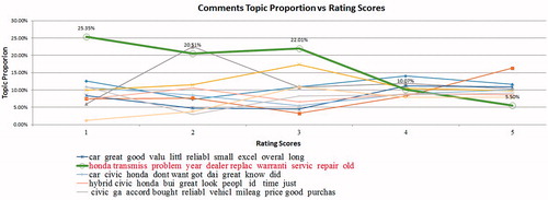
Therefore, the decision variables associated with transmission design (Xs) are targeted for prioritization in design changes. The strata (rating scores) for different topics are the “variable containers” (De Mast and Trip 2007), and the causal relationship is suggested through the variations of topic proportions across strata.

Example 3: Quality improvement for the Ford F-150

This example is also based on Consumer Reports data providing 369 records for the Ford F-150. The example involves the years 2000–2010 and the actual numbers of recalls from 2000–2010 during those years. Sentiment analysis is done for each of the 369 comments in the consumer report using Eq. [3](3) $$S=\ln \left(0.5+P\right)-\ln \left(0.5+N\right).$$(3) tabulated using software from CX Data Science. By tabulated recall counts against the sentiment scores from the report text, a relationship can be established. The linear relationship of sentiment scores and the actual number of recalls is shown in Figure 3(a). From this, the following linear regression model is derived: (5) $$\widehat{S}=0.4950-0.03767\mathrm{ }(\#\text{Recalls})$$(5)

Figure 3. Linear regression model and residual plots for comments sentiment scores.

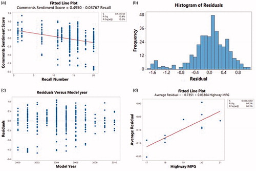
The sentiment score is predicted to be high when the recall number is low. The histogram of residuals of the linear regression relationship is plotted in Figure 3(b). Based on the bimodality of the distribution for the residual plot, it seems that there is likely another cause for the low scores in addition to recalls. This shows the evidence of presence of a “lurking variable” worth investigating for the quality improvement.

Plotting the residuals by time strata (model year) in Figure 3(c) provides information about the timeliness of the missing cause. Most importantly, perhaps, the residual plot indicates that the causes do not endure to the latest model years.

The highest negative sentiment score residuals are found in 2000 and 2002. Exploration of the comments in 2000 and 2001 shows that many are about poor gas mileage. In 2000, the trucks miles-per-gallon averaged only 13 city/17 highway miles per gallon (MPG). From 2002 to 2007, truck MPG improved resulting in fewer customer complaints about this shortcoming. This is reflected in the less negative residuals in 2003–2007. After 2008, fuel consumption improved further, reaching more than 20 MPG on highways. Figure 3(d) shows the linear relationship between yearly average residuals of the comments sentiment score versus MPG. Combining both the inferences from Figure 3(b) and (d), it is suggested that further improvements might not reduce negative sentiment after 2010 since mean negative sentiment is dominated by recalls.

Example 3 illustrates how ETDA can provide insights relevant to design teams and related prioritization. This is a case in which text data is used to help discover dependent variables (Xs) by focusing on one or more time intervals in the data. The bimodality distribution of residuals deviates from the expected normal distribution of linear regression residuals. To summarize, an approximate model of sentiment is first generated using recall counts. Then, inspecting the residuals, an additional factor relating to miles per gallon is hypothesized and may lead to a refined model. Further investigation suggests that the effects for the F-150 associated with gas mileage might only be operating in the early years of the time period studied.

Example 4: Cyber attack incidents related to Heartbleed

This example uses the cyber security Twitter account data detailed in Allen et al. (2017) and Sui et al. (2015). A large Midwest institution suffered from a high number of cyber-attacks and experienced a sudden computer intrusion hike in April 2014. To leverage ETDA for the quality hypothesis generation, inquirers collected 16,047 Tweets from January 2014 to December 2014 from 16 Twitter accounts of noted cyber experts. The collapsed Gibbs Sampling Topic Modeling techniques is used to break the Tweets into 10 topics. For each topic, the topic proportions are acquired for each month and the differences from the previous month are charted in the running time chart in Figure 4. The third topic in the legend is associated with the grey-colored line and references the famous “Heartbleed” vulnerability. Retweets (rt) is a common and potentially uninformative common term. Adding “rt” to the “stop word” list may be desirable so that it can be removed from consideration in the analysis.

Figure 4. Topic proportion differences (month-to-month) vs. months.

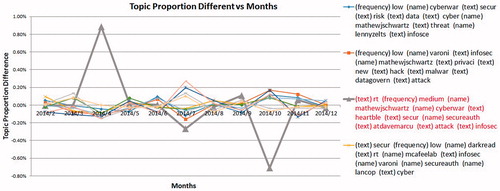
Cluster or topic 3 experiences a sudden increase in topic proportion in April 2014 and a sudden decrease in topic proportion in October 2014, while other topics’ changes are relatively constant, fluctuating around zero. This pattern is consistent with the timing of the public disclosure of the vulnerability, “Heartbleed”, on April 1, 2014. This vulnerability resulted from a lack of bounds in memory allocations for operating systems, which allowed large amounts of information to be stolen from any susceptible computer.

Upon this disclosure, many hackers made use of the vulnerability before a patch could be created resulting, among other disruptions, in the roughly 400% increase in cyberattacks experienced by the large Midwest institution in the month of April 2014. The sudden increase in topic proportion that month shows a surge in discussion of the issue on Twitter. Figure 4 suggests both that the uptick in incidents might likely have been caused by Heartbleed and that the issues was resolved by September.

Example 4 also shows how cluster posterior probability estimates can provide reference values for comparisons between clusters. General reference comparisons lead to the principle:

D3. Look for deviations or variations from other references which could be other fields.

For data with multiple fields, a comparison of causal relationships across and within fields can be beneficial. If one or some of the fields behave differently from most other fields, the salient features of those abnormal fields could be explored for quality hypothesis generation.

D4. Look for salient feature based on prior perceptions, rules, or knowledge.

Prior experience or field knowledge can help to identify salient features. In Example 2, the finding that a topic has a high proportion of low ratings and a low proportion of high ratings, obviously suggests it is worth exploring for salient features related to quality.

Example 5 illustrates the use of context knowledge to generate hypotheses in a customer support feedback call center. In this case, the context knowledge enters explicitly in the clustering process. Also, it enters in identifying the subsystems that should likely be prioritized for additional study.

Example 5: Call center improvement

Allen et al. (2016) presented a call center service improvement problem to an insurance company. Using 2,378 records of conversations between the service representatives and callers, Allen et al. (2016) extended and applied the topic modeling with subject matter refined topic (SMERT) to acquire 10 topics. Applying this variation of LDA allowed a process of topic editing and refinement of the topic definitions. Mulaik (1985) argued that iterative interpretation of salient features is often crucial in exploring problems. The incorporation of subject matter expertise could greatly help with the interpreting through subject matter knowledge. This combination could further achieve a more definitive result relating to the root cause of problems under study. The estimated topic proportions that emerged are shown in Figure 5.

Figure 5. Call center clusters from SMERT model with manually entered interpretations.

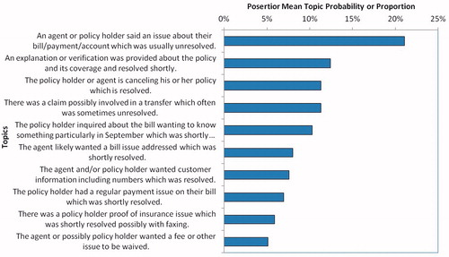
By describing the topics as sentences instead of word lists, the result is directly relevant to call center operations. Automatic answering logic can then target the top issues. This logic could permit reducing the burden on the order answerers. For example, improved logic relating to bills and payment could address over 20% of the call volume. Further, by studying Figure 5, we estimate that improved automatic information and verification (relating to topic 2) might reduce the call volume by approximately 12%.

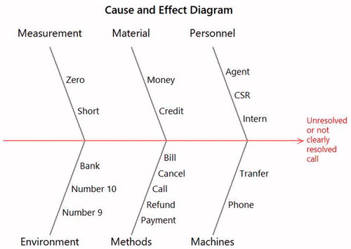
Analyzing the top topic (topic #1) by proportion further can suggest additional salient features and suggest more detailed causal hypotheses. Topic #1 relates to a certain type of unresolved calls and therefore a quality-related problem. To gain insights into addressing this problem, the word cloud software from Davies (2017) is applied in Figure 6. Figure 6(a) shows the word cloud from all the call center data. Figure 6(b) shows a word cloud from an artificial corpus created by expressing words in proportion to the posterior mean topic probability estimates. From this comparison, a hypothesis is generated that the cause of the problem relates to note-taking involving the customer service representative (CSR) and agents. Similarly, the words with the highest posterior mean probabilities in this topic probability can be used to populate a cause and effect matrix in Figure 7. The result might be interpreted as a need to improve the specific methods: billing, canceling, refunds, and payments. Therefore, the results illuminate the proportion of each of the common issues that can be addressed and relatively specific hypotheses about how to make improvements.

Figure 6. (a) Word cloud of all call center data and (b) word cloud of words associated with topic #1.

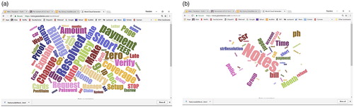
Figure 7. Cause and effect matrix populated using the top words from topic #1.

Final remarks

In this article, we describe how the exploratory (EDA) framework of De Mast and Trip (2007) applies to text data. The resulting ETDA principles are developed using examples from real-world quality improvement projects. The purposes of the overall analysis can be identified first. Then, ETDA involves an initial “preprocessing” step which could involve clustering, sentiment analysis, or another procedure which transforms the text into quantitative inputs for further analysis. The first set of proposed principles and methods (A) primarily relates to identification of key input and output variables. The second set relates to using transparent word counts or weighted counts (B) and the third relates to studying the nature of the variation (C). Methods for investigating deviations from a standard are then studied (D) and methods for exploring the salient features are described (E).

While automated algorithms could help in certain steps such as text data analysis and display (Step 2) and identification of salient features (Step 3), it is difficult to imagine that interpretation (Step 4) could easily be automated. In our examples, it required intuition to relate the topics or semantic relationships with possible causes of interest to practitioners. Automatic preprocessing, however, is perhaps the main motivation for the use of text modeling methods with millions of Tweets, for example, being transformed in seconds into a Pareto chart as in Figure 1.

Also, it should be noted that ETDA only generates hypotheses and not confirmed results. Additional data collection and CDA are generally needed to generate facts about the causes of problems. The subjectivity of text, clustering, and semantic analyses only compound the inherent indeterminacy of EDA. Therefore, if the results of ordinary EDA are regarded skeptically, this skepticism should likely be deepened for EDTA.

Data available for ETDA are growing and likely compromises most of all data. Yet, there is the common issue that available data might not be representative of the relevant populations. In Example 2, inputs from Consumer Reports members may not be representative of the owner population. Therefore, there is a need to combine EDTA with other statistical methods in the analysis process. Further, while there is no clear problem with using the same data to generate and test hypotheses, the subjectivity of text data suggest an additional burden in collecting new data for confirmation will often be needed. Text data might rarely seem appropriate for proving physical effects in a manner like other types of engineering data.

We developed ETDA with various forms of text inputs to quality and design engineering in mind: surveys, complaint transcripts, customer ratings, or maintenance squawks. We hope that the principles, methods, and diagrams introduced here may become a standard part of the analysis process for these types of data. Then, more promising hypotheses about the causes for quality problems and avenues for improvements may be generated in part because the clinical “mind set” commonly in use relating to other types of data can be extended to text data.

Many topics are available for future research. Example 4 illustrates the partial exploitation of the document topic matrix (DTM) from LDA to visualize the time series of issues. Other possibilities for exploiting the DTM matrices include clustering the documents and retrieving documents primarily relevant to specific topics which can be explored. Additional investigations can illuminate relevant routines in software familiar to quality professionals including in R, Python, SAS, JMP, and SPSS Modeler.

Acknowledgments

We appreciate Mrs. Jodie Allen for her help in proofreading. Consumer Reports generously provided the data for Examples 1–3. Major Nate Parker provided encouragement. The anonymous reviewers provided key ideas about additional analyses relating to topic modeling and for improving the organizational structure of the paper.

Additional information

Funding

NSF grant #1409214 partially supported this work.

Notes on contributors

Theodore T. Allen

Theodore T. Allen is an associate professor of Integrated Systems Engineering at The Ohio State University and the founder and president of factSpread. He received his Ph.D. in Industrial Operations Engineering from the University of Michigan. He is the author of over 50 peer reviewed publications including two textbooks. He is the president of the INFORMS social media analytics section and a simulation area editor for Computers & Industrial Engineering (IF: 3.2).

Zhenhuan Sui

Zhenhuan Sui received his Ph.D. in Integrated Systems Engineering at The Ohio State University in 2017. His interests relate to natural language processing (NLP), data-driven banking decision-making, hierarchical Bayesian models, and machine learning algorithms.

Kaveh Akbari

Kaveh Akbari graduated with his M.S. in Integrated Systems Engineering department at The Ohio State University. His interests include decision making under uncertainty in energy systems, large-scale optimization algorithms and natural language processing (NLP).

Appendix

The latent Dirichlet allocation (LDA) model is a probabilistic model of a corpus. This statistical model is proposed in Blei et al. (2003). In LDA, documents are random mixtures over latent topics and each topic is characterized by a distribution over the words. Assume that $w_{d,j}$ is the $j^{}$th word in dth document with d = 1, …, D and j = 1, …, N_d, where D is the number of documents, and N_d is the number of words in the dth document. Therefore, $w_{d,j}\in \{1,\dots ,W\}$, where $W$ is the number of distinct words in all documents. The clusters or “topics” are defined by the estimated probabilities, ${\widehat{\varphi }}_{t,c}$, which signifies a randomly selected word in cluster t = 1, …, T (on that topic) achieving the specific value c = 1, …, W. Also, ${\widehat{\theta }}_{d,t}$ represents the estimated probability that a randomly selected word in document d is assigned to cluster or topic t. The model variables $z_{d,j}$ are the cluster assignments for each word in each document, d = 1, …, D and j = 1, …, N_d. Then, the joint probability of the word $w_{d,j}$ and the parameters to be estimated, ($z_{d,j},\mathrm{ }{\theta }_{d,t},{\varphi }_{t,c}$), is: $$P\left(w_{d,j},z_{d,j},\mathrm{ }{\theta }_{d,t},{\varphi }_{t,c}|N_d,\alpha ,\beta ,\mathrm{ }d=1,\dots ,D,\mathrm{ }t=1,\dots ,T,c=1,\dots ,W\right)=\left[\prod _{t=1}^T\frac{\Gamma \left({\sum }_{c=1}^W\beta \right)}{\prod _{c=1}^{WC}\Gamma \left(\beta \right)}\prod _{c=1}^W{\varphi }_{t,c}^{\beta -1}\right]\left[\prod _{d=1}^D\frac{\Gamma \left({\sum }_{c=1}^W\alpha \right)}{\prod _{c=1}^{WC}\Gamma \left(\alpha \right)}\prod _{t=1}^T{\theta }_{d,t}^{\alpha -1}\right]\times \left[\prod _{d=1}^D\prod _{t=1}^T{\theta }_{d,t}^{n_t^{\left(d\right)}}\right]\times \left[\prod _{t=1}^T\prod _{c=1}^W{\varphi }_{t,c}^{n_t^{\left(c\right)}}\right]$$ where $\Gamma \left(\dots \right)$ is the gamma function and: (6) $$n_t^{\left(d\right)}=\sum _{j=1}^{N_d}\sum _{c^{\mathrm{\prime }}=1}^{W}I\left(z_{d,j}=t\mathrm{ }\&\mathrm{ }c=c^{\mathrm{\prime }}\right)\text{ and }{n}_t^{\left(c\right)}=\sum _{d=1}^D\sum _{j=1}^{N_d}I\left(z_{d,j}=t\mathrm{ }\&{\mathrm{ }w}_{d,j}=c\right)$$(6) and where $I(\dots )$ is an indicator function giving 1 if the equalities hold and zero otherwise.

Note Eq. [6](6) $$n_t^{\left(d\right)}=\sum _{j=1}^{N_d}\sum _{c^{\mathrm{\prime }}=1}^{W}I\left(z_{d,j}=t\mathrm{ }\&\mathrm{ }c=c^{\mathrm{\prime }}\right)\text{ and }{n}_t^{\left(c\right)}=\sum _{d=1}^D\sum _{j=1}^{N_d}I\left(z_{d,j}=t\mathrm{ }\&{\mathrm{ }w}_{d,j}=c\right)$$(6) is a simple representation of human speech in which words, ${\mathrm{ }w}_{d,j}$, and topic assignment,$\mathrm{ }{z}_{d,j}$, are both multinomial draws associated with the given topics. The probabilities ${\varphi }_{t,c}$ that define the topics are also random with a hierarchical distribution. The estimates that are often used for these probabilities are Monte Carlo estimates for the posterior means of the Dirichlet distributed probabilities ${\widehat{\theta }}_{d,t}$ and ${\widehat{\varphi }}_{t,c}$, produced by low values or diffuse prior parameters $\alpha$ and $\beta$.

To estimate the parameters in the LDA model in Eq. [6](6) $$n_t^{\left(d\right)}=\sum _{j=1}^{N_d}\sum _{c^{\mathrm{\prime }}=1}^{W}I\left(z_{d,j}=t\mathrm{ }\&\mathrm{ }c=c^{\mathrm{\prime }}\right)\text{ and }{n}_t^{\left(c\right)}=\sum _{d=1}^D\sum _{j=1}^{N_d}I\left(z_{d,j}=t\mathrm{ }\&{\mathrm{ }w}_{d,j}=c\right)$$(6) , “collapsed Gibbs” sampling (Teh et al. 2007; Griffiths and Steyvers 2004) is widely used. First the values of the topic assignments for each word $z_{d,j}$ are sampled uniformly. Then, iteratively, multinomial samples are drawn for each topic assignment $z_{d,j}$ iterating through each document d and word j using the last iterations of all other assignments $z_{-\left(d,j\right)}$. The multinomial draw probabilities are (7) $$P\left(z_{d,j}=t|{d,j,z}_{-\left(\mathit{d},\mathit{j}\right)},w_{d,j}\right)\propto \left(\frac{n_t^{\left(w_{d,j}\right)}-I\left(z_{d,j}=t\mathrm{ }\right)+\beta }{n_t^{(·)}-I\left(z_{d,j}=t\mathrm{ }\right)+W\beta }\right)\left(\frac{n_t^{\left(d\right)}-I\left(z_{d,j}=t\mathrm{ }\right)+\alpha }{n_{·}^{\left(d\right)}-1+T\alpha }\right)$$(7) where $n_t^{(w_{d,j})}={\sum }_{d^{\mathrm{\prime }}=1}^D{\sum }_{j^{\mathrm{\prime }}=1}^{N_d}I\left(z_{d^{\mathrm{\prime }},j^{\mathrm{\prime }}}=t\mathrm{ }\&{\mathrm{ }w}_{d^{\mathrm{\prime }},j^{\mathrm{\prime }}}=w_{d,j}\right)$, $$n_t^{\left(·\right)}={\sum }_{d^{\mathrm{\prime }}=1}^D{\sum }_{j^{\mathrm{\prime }}=1}^{N_d}I\left(z_{d,j^{\mathrm{\prime }}}=t\mathrm{ }\right)$$ $$n_t^{\left(d\right)}=\sum _{j=1}^{N_d}\sum _{c^{\mathrm{\prime }}=1}^{W}I\left(z_{d,j}=t\mathrm{ }\&\mathrm{ }c=c^{\mathrm{\prime }}\right)$$ and $$n_{·}^{\left(d\right)}=\sum _{t^{\mathrm{\prime }}=1}^T\sum _{j^{\mathrm{\prime }}=1}^{N_d}I\left(z_{d,j^{\mathrm{\prime }}}=t\right)$$

In words, each word is randomly assigned to a cluster with probabilities proportional to the counts for that word being assigned multiplied by the counts for that document being assigned. After M iterations, the last set of topic assignments generate the estimated posterior means using: (8) $${\widehat{\varphi }}_{t,c}=\frac{n_t^{\left(c\right)}+\beta }{n_t^{(·)}+W\beta }$$(8)

And the posterior mean topic definitions using (9) $${\widehat{\theta }}_{d,t}=\frac{n_t^{\left(d\right)}+\alpha }{n_{·}^{\left(d\right)}+T\alpha }$$(9)

Therefore, if words are assigned commonly to certain topics by the Gibbs sampling model, their frequency increases the posterior probability estimates both in the topic definitions ${\widehat{\varphi }}_{t,c}$ and the document probabilities ${\widehat{\theta }}_{d,t}$.

References

- Allen, T. T., N. Parker, and Z. Sui. 2016. Using innovative text analytics on a military specific corpus. 84th Military Operations Research Society (MORS) Symposium, Quantico, VA, June, 170. https://www.jstor.org/stable/24910203?seq=1#page_scan_tab_contents.
- Allen, T. T., Z. Sui, and N. L. Parker. 2017. Timely decision analysis enabled by efficient social media modeling. Decision Analysis 14 (4):250–260. doi:10.1287/deca.2017.0360.
- Allen, T. T., and H. Xiong. 2012. Pareto charting using multifield freestyle text data applied to Toyota Camry user reviews. Applied Stochastic Models in Business and Industry 28 (2):152–163. doi:10.1002/asmb.947.
- Allen, T. T., H. Xiong, and A. Afful-Dadzie. 2016. A directed topic model applied to call center improvement. Applied Stochastic Models in Business and Industry 32 (1):57–73. doi:10.1002/asmb.2123.
- Bisgaard, S. 1996. The importance of graphics in problem solving and detective work. Quality Engineering 9 (1):157–162. doi:10.1080/08982119608919028.
- Blei, D. M., A. Y. Ng, and M. I. Jordan. 2003. Latent Dirichlet allocation. Journal of Machine Learning Research 3:993–1022. doi:10.1162/jmlr.2003.3.4-5.993.
- Davies, J. 2017. https://www.jasondavies.com/wordcloud/ (accessed February 2017).
- De Mast, J., and A. Trip. 2007. Exploratory data analysis in quality-improvement projects. Journal of Quality Technology 39 (4):301–311. doi:10.1080/00224065.2007.11917697.
- Feldman, R., and J. Sanger. 2007. The text mining handbook: advanced approaches in analyzing unstructured data. Cambridge, UK: Cambridge University Press.
- Good, I. J. 1983. The philosophy of exploratory data analysis. Philosophy of Science 50 (2):283–295. doi:10.1086/289110.
- Griffiths, T. L., and M. Steyvers. 2004. Finding scientific topics. Proceedings of the National Academy of Sciences 101 (Supplement 1):5228–5235. doi:10.1073/pnas.0307752101.
- Hoaglin, D. C., F. Mosteller, and J. W. Tukey. 1983. Understanding robust and exploratory data analysis. New York, NY: Wiley.
- Liu, B. 2012. Sentiment analysis and opinion mining. Synthesis Lectures on Human Language Technologies 5 (1):1–167. doi:10.2200/S00416ED1V01Y201204HLT016.
- Mulaik, S. A. 1985. Exploratory statistics and empiricism. Philosophy of Science 52 (3):410–430. doi:10.1086/289258.
- Niiniluoto, I. 1999. Defending abduction. Philosophy of Science 66:S436–S451. doi:10.1086/392744.
- Pang, B., and L. Lee. 2008. Opinion mining and sentiment analysis. Foundations and Trends in Information Retrieval 2 (1–2):1–135. doi:10.1561/1500000011.
- Parker, N., T. T. Allen, and Z. Sui. 2017. K-Means Subject Matter Expert Refined Topic Model Methodology. (No. TRAC-M-TR-17-008). TRAC-Monterey Monterey, United States. http://www.dtic.mil/docs/citations/AD1028777
- Porter, M. F. 1980. An algorithm for suffix stripping. Program 14 (3):130–137. doi:10.1108/eb046814.
- Shewhart, W. A. (1939) 1986. Statistical method from the viewpoint of quality control. Washington: The Graduate School of the Department of Agriculture. Reprint, New York: Dover Publications.
- Shewhart, W. A. 1931. Economic control of quality of manufactured product. Princeton: Van Nostrand Reinhold. doi:10.2307/2277676.
- Sui, Z. 2017. Hierarchical Text Topic Modeling with Applications in Social Media-Enabled Cyber Maintenance Decision Analysis and Quality Hypothesis Generation. PhD dissertation, The Ohio State University, Integrated Systems Engineering. http://rave.ohiolink.edu/etdc/view?acc_num=osu1499446404436637
- Sui, Z., and T. T. Allen. 2016. NLP, LDA, SMERT, k-means and Efficient Estimation Methods with Military Applications. INFORMS Annual Meeting, Nashville, Tennessee, November.
- Sui, Z., D. Milam, and T. T. Allen. 2015. A visual monitoring technique based on importance score and Twitter, 319. INFORMS Annual Meeting, Philadelphia, Pennsylvania, November.
- Teh, Y. W., D. Newman, and M. Welling. 2007. A collapsed variation Bayesian inference algorithm for latent Dirichlet allocation. Advances in Neural Information Processing Systems 19:1353–1360. doi:10.1.1.85.9574.
- Tukey, J. W. 1977. Exploratory data analysis. Reading, PA: Addison-Wesley.
- Turney, P. D. 2002. Thumbs up or thumbs down?: Semantic orientation applied to unsupervised classification of reviews. Proceedings of the 40th Annual Meeting on Association for Computational Linguistics, 417–424. doi:10.3115/1073083.1073153.