Network based credit risk models

Abstract

Peer-to-Peer lending platforms may lead to cost reduction, and to an improved user experience. These improvements may come at the price of inaccurate credit risk measurements, which can hamper lenders and endanger the stability of a financial system. In the article, we propose how to improve credit risk accuracy of peer to peer platforms and, specifically, of those who lend to small and medium enterprises. To achieve this goal, we propose to augment traditional credit scoring methods with “alternative data” that consist of centrality measures derived from similarity networks among borrowers, deduced from their financial ratios. Our empirical findings suggest that the proposed approach improves predictive accuracy as well as model explainability.

Keywords:

• credit scoring models
• network models
• peer-to-peer lending

Introduction

In the recent years, the emergence of financial technologies (fintechs) has redefined the roles of traditional intermediaries and has introduced many opportunities for consumers and investors. Here we focus on peer-to-peer (P2P) online lending platforms, which allow private individuals to directly make small and unsecured loans to private borrowers. The recent growth of peer to peer lending is due to several “push” factors. First, when compared to classical banks, P2P platforms have much lower intermediation costs. Second, the evolution of big data analytics enables them to provide banking services that can improve personalization and, therefore, user experience. A third push factor is the presence of favorable, or absent, regulation. For instance, the European Payment Service Directive (PSD2) which is going to disclose bank clients’ account information, previously reserved to banks, also to fintechs, through application payment interfaces that take consumer’s consent and ethics into account.

P2P lending business models vary in scope and structure: a comprehensive review is provided by Claessens et al. (2018). Here we specifically refer to the platforms that enable lending to small and medium enterprises (SME), as in the paper by Giudici and Hadji-Misheva (2017).

A key point of interest to assess the sustainability of P2P business lenders is to evaluate the accuracy of the credit risk measurements they assign to the borrowers. While both classic banks and P2P platforms rely on credit scoring models for the purpose of estimating the credit risk of their loans, the incentive for model accuracy may differ significantly. In a bank, the assessment of credit risk of the loans is conducted by the financial institution itself which, being the actual entity that assumes the risk, is interested to have the most accurate possible model. In a P2P lending platform, credit risk of the loans is determined by the platform but the risk is fully borne by the lender. In other words, P2P lenders allow for direct matching between borrowers and lenders, without the loans being held on the intermediary’s balance sheet (Milne and Parboteeah 2016).

From a different perspective, while in classical banking a financial institution chooses its optimal tradeoff between risks and returns, subject to regulatory constraints, in P2P lending a platform maximizes its returns, without taking care of the risks which are borne by the lenders.

Another factor that penalizes the accuracy of P2P credit scoring models is that they often do not have access to borrowers’ data usually employed by banks, such as account transaction data, financial data and credit bureau data.

For these reasons, the accuracy of credit risk estimates provided by P2P lenders may be poor. However, P2P platforms operate as social networks, which involve their users and, in particular, the borrowers, in a continuous networking activity. Data from such activity can be leveraged not only for commercial purposes, as it is customarily done, but also to improve credit risk accuracy.

We believe that the usage of “alternative” data, consisting of networking information, can offset the mentioned disadvantages and can improve credit risk measurement accuracy of P2P lenders. From a regulatory viewpoint, this implies that P2P lenders should not be penalized, with stringent rules, or with the imposition of high capital buffers.

Classical banks have, over the years, segmented their reference markets into specific territorial areas and business activities, increasing the accuracy of their ratings but, on the other hand, increasing concentration risks. Classical banks automatically receive data that concern the transaction of each company with the bank and can easily obtain further information about the financial situation and the payment history of each company.

Differently, P2P platforms are based on a “universal” banking model, fully inclusive, without space and business type limitations, that benefits from diversification. P2P platforms automatically receive data from the participants in the platforms, that concern transactions and/or relationships of each company not just with the platform but also with each other. Provided that enough companies populate the platform, the resulting networking data are richer than the that of banks as it contains more information. In particular, it contains data about how companies interact with each other, in terms of payments, demand and supply chains, control and governance.

The latter information can be used for the purpose of creating a network model which can quantify how borrowers are interconnected with each other. A model that can be employed to improve loan default predictions.

Our aim is to build a network model from the publicly available platform data. A model that can be applied by regulators and supervisors and, more generally, for the external evaluation of the credit risk generated by a P2P lender.

To achieve this goal, we inevitably face the problem that, typically, networking data are available internally to the platform but not externally. This also because, differently from the traditional baking sector, the fintech sector is still largely unregulated.

To overcome this issue, one approach is building correlation networks based on the pairwise correlations that can be deduced from the time series of publicly available balance sheets of SMEs, possibly standardized according to common accounting standards. Correlation network models have indeed proven to be effective, even in the interbank lending context, where actual network data are usually available (see e.g., Brunetti et al. 2015; Giudici, Sarlin, and Spelta 2017) and, for this reason, we rely on them.

Correlation network models can combine the rich structure of financial networks (see, e.g., Battiston et al. 2012; Lorenz, Battiston, and Schweitzer 2009; Mantegna 1999) with a parsimonious approach based on the dependence structure among market prices. Important contributions in this framework are Billio et al. (2012); Hautsch, Schaumburg, and Schienle (2015), Ahelegbey, Billio, and Casarin (2016), Giudici and Spelta (2016), and Giudici and Parisi (2018), who propose measures of connectedness based on similarities, Granger-causality tests, variance decompositions and partial correlations between market price variables.

Our model extends the above approaches, as it employs: i) centrality measures obtained from the similarity networks that emerge between SME companies and ii) a dependency model, based on logistic regression, that allows embedding network information into an explainable logistic regression model that is not just descriptive but also predictive.

To summarize, the main methodological contributions of this article are: i) a novel network model between economic entities (borrowers) using financial variables, rather than market prices; ii) the insertion of summary information on how SMEs are connected to each other in the scoring models, making them predictive.

Our empirical findings show that the proposed scoring model, enhanced by similarity networks, considerably improves the predictive accuracy of credit scoring model, and it helps its explainability, even to non-technical experts.

We remark that our work is related to two main other recent research streams. First, some authors have carried out investigations on the accuracy of credit scoring models of P2P platforms. We improve these contributions with a more formal statistical testing procedure and, furthermore, with the extension to SME lending. Second, our network models relate to a recent and fast expanding line of research which focuses on the application of network analysis tools, for the purpose of understanding flows in financial markets, as in the papers of Allen and Gale (2000), Leitner (2005) and Giudici and Spelta (2016). We improve these contributions, extending them to the P2P context and linking network models, that are often merely descriptive, with logistic regression models, thus providing a predictive framework.

The article is organized as follows. Section 2 explains the methodology we propose, to achieve the stated research goals, Section 3 presents the data we have considered, whereas Section 4 presents the results obtained applying the developed methods to the data. We conclude with a final discussion.

Methodology

Scoring models

The most popular statistical model to estimate the probability of default of a borrower is the logistic regression. In the context of P2P lending, logistic regression has been used by Barrios, Andreeva, and Ansell (2014), Emekter et al. (2015) and Serrano-Cinca et al. These authors classify P2P borrowers in two groups, characterized by a different history of payments of the loans that were funded through the platform: 0 = active (all loans have been paid on time); 1 = default (at least one loan has not been paid on time).

A logistic regression model estimates the probability that a borrower defaults, using data on a set of borrower specific variables. More formally: $$\mathit{ln}\left(\frac{p_i}{1-p_i}\right)=\alpha +\sum _j{\beta }_j{x}_{\mathit{ij}},$$ where, for each borrower $i=(1,\dots ,I)$: p_i is the probability of default; $x_i=(x_{i1},\dots ,x_{\mathit{ij}},\dots ,x_{\mathit{iJ}})$ is a vector of borrower-specific explanatory variables; the intercept parameter α, and the regression coefficients β_j, for $j=1,\dots ,J$, are unknown, and need to be estimated from the available data.

From the previous expression the probability of default of each borrower can be obtained as: $$p_i=\frac{1}{1+e^{\alpha +\sum _j{\beta }_j{x}_{\mathit{ij}}}},$$ the credit score of i, whose default status will be predicted to be 1 or 0 depending on whether p_i exceeds or not a set threshold θ. Common choices for the threshold are $\theta =.5$ or $\theta =d/I$, with d the observed number of defaults.

The previous model, once estimated on a training sample, can be used to predict the probability of default of a new loan, so that lenders can decide whether to invest on it, or not. This decision crucially depends on the accuracy of the prediction which, in turn, depends on the validity of the employed model.

As discussed in the introduction, peer to peer lending platforms may underestimate the probability of default of a loan, because of a high set threshold or because of a lack of explanatory variables data. While the choice of a threshold remains a subjective decision, the improvement of the explanatory variables can be achieved exploiting borrowers’ networking data. We believe that incorporating network information into a credit scoring model could improve default predictive accuracy. This requires building an appropriate network analysis model.

Network models

Network analysis models have become increasingly recognized as a powerful methodology for investigating and modeling interactions between economic agents (Minoiu and Reyes 2010). In particular, correlation network models, that rely on correlations between the units of analysis (borrowers, in our context), according to a given set of statistical variables, have been proposed by Giudici, Sarlin, and Spelta (2017), in the context of interbank lending. The authors compare correlation networks with “physical” networks, based on actual transactions, and show that they can achieve comparable predictive performances.

Mathematically, correlation network models are related to graphical models. A graphical model can be defined by a graph $\mathcal{G}=(\mathcal{V},\mathcal{W})$ where V is a set of vertices (nodes) and $W=V\times V$ is a set of weights (links) between all the vertices.

In a graphical Markov model (see e.g., Lauritzen 1996) the weight set specializes to an edge set E, that describes whether any pair of vertices (i, j) is connected $(i,j)\in E$ or not $(i,j)\notin E$. A graphical Markov model can be fully specified by an adjacency matrix, A. The adjacency matrix A of a vertex set V is the I × I matrix whose entries are a_ij = 1 if $(i.j)\in E$, and 0 otherwise.

From a statistical viewpoint, each vertex $v\in V$ in a graphical Markov model can be associated with a random variable X_v. When the vector of random variables $(X_v,v\in V)$ follows a multivariate Gaussian distribution, the model becomes a graphical Gaussian model, characterized by a correlation matrix R which can be used to derive the adjacency matrix. This because the following equivalence holds: $$(i,j)\notin E\iff {(R^{-1})}_{\mathit{ij}}=0,$$ which states that a missing edge between vertex i and vertex j in the graph is equivalent to the partial correlation between variables X_i and X_j being equal to zero.

Building on the previous equivalence, a graphical Gaussian model is able to learn from the data the structure of a graph (the adjacency matrix) and, therefore, the dependence structure between the associated random variables. In particular, an edge can be retained in the model iff the corresponding partial correlation is significantly different from zero.

In a network analysis model (see e.g., Barabasi 2016), the set W is a set of weights, which usually connect each variable with all others. In other words, the graph is fully connected.

From a statistical viewpoint, each vertex $v\in V$ in a network analysis model is associated with a statistical unit, and each weight describes an observed relationship between a pair of units, such as a quantity of goods or a financial amount. While the adjacency matrix in a graphical Markov models is symmetric, the weight matrix does not need to be so. For instance, in interbank lending, which is one of the main application of network analysis to the financial domain, the weights are financial transactions, with w_ij indicating how much i lends to j and w_ji indicating how much j lends to i. The aim of a network analysis model is not to learn from the data the structure of a graph but, rather, to summarize a complex structure, described by a graph, in terms of summary measures, or topological properties.

A correlation network model (see e.g., Giudici, Sarlin, and Spelta 2017; Mantegna 1999) is a network analysis model for which the weights are not directly observed, but are calculated as correlations between the observed values of a given random vector X_v, $(1, \dots ,N$), for each pair of statistical units.

Note that correlation network models are similar to graphical Markov models, as they are based on statistical relationships between variables. However, differently from graphical Markov models, (and similarly to network analysis models) they relate units, rather than variables, and they are based on correlations, rather than on partial correlations.

Note also that correlation networks are different from financial networks, the network analysis models typically considered in the financial literature (see e.g., Battiston et al. 2012). Financial networks are based on data that describe the actual financial flows between each pair of borrowers, in a given time period. If this information is available we could use them as weights, directly. However, this is an approach that we cannot follow when the transactions between borrowers are not available or, even when they are, when they lead to a sparse weight matrix. In addition, Giudici, Sarlin, and Spelta (2017) showed, in the context of international banking, that, even when available and not sparse, financial networks can be matched, or even improved, in terms of predictive performance, by correlation networks.

In the peer to peer lending context, each vertex of a correlation network corresponds to a borrower company; while each edge represents a correlation (a distance) between any two companies.

More precisely, suppose we have financial information about the borrowing companies collected in a vector ${\mathbf{x}}_n$, extracted from the financial ratios of n companies in a given year. We follow the convention of credit scoring models and consider the financial ratios of the year that precedes the observation of whether a company defaults or not.

We can define a metric that provides the relative distance between any two companies by applying the standardized Euclidean distance between each pair $({\mathbf{x}}_i,{\mathbf{x}}_j)$ of institutions feature vectors. More formally, we define the pairwise distance $d_{i,j}$ as: [1] $$d_{i,j}=({\mathbf{x}}_i-{\mathbf{x}}_j){\mathbf{\Delta }}^{-1}({\mathbf{x}}_i-{\mathbf{x}}_j)\prime$$[1] where $\mathbf{\Delta }$ is a diagonal matrix whose i-th diagonal element is $S_i^2$, being S the vector of standard deviation. Namely, each coordinate difference between pairs of vectors $({\mathbf{x}}_i-{\mathbf{x}}_j)$ is scaled by dividing by the corresponding element of the standard deviation. The distances can be embedded into a N × N dissimilarity matrix D such that the closer the companies i, j features are in the Euclidean space, the lower the entry $d_{i,j}$. In other words, the stronger the similarity (i.e., the force that connects two companies’ characteristic vectors), the weaker the link connecting the institutions. Pairs of companies that are dissimilar receive higher weights since they are placed far away from each other, while values approaching zero are assigned to pairs with highly similar characteristics.

Although D can be informative about the distribution of the distances between the companies, the fully-connected nature of this set does not help to find out whether there exist dominant patterns of similarities between institutions. Therefore the extraction of such patterns demands a representation of the system where sparseness replaces completeness in a suitable way. To accomplish this purpose we can follow the Minimal Spanning Tree (MST) approach introduced by Mantegna (1999).

To find out the MST representation of the system we use the Prim algorithm where we start with any single node and we add new nodes one by one to the tree so that at each step, the node closes to the nodes includes so far, is added.

Network centralities

Understanding the structure of a correlation network, and in particular determining which nodes act as hubs or as authorities, is key to understand the origin of companies failures and to inform policymakers on how to prepare and recover from adverse shocks hitting an economic system.

The research in network theory has dedicated a huge effort to developing measures of interconnectedness, related to the detection of the most important players in a network. The idea of centrality was initially proposed in the context of social systems, where a relation between the location of a subject in the social network and its influence on group processes was assumed. Various measures of centrality have been proposed in network theory, including local measures, such as the degree centrality, which counts the number of neighbors of a node; or measures based on the global spectral properties of the graph. The latter include the eigenvector centrality (Bonacich 2007), Katz centrality (Katz 1953), PageRank (Brin and Page 1998), hub and authority centralities (Kleinberg 1999). These measures are feedback centrality measures and provide information on the position of each node relative to all other nodes.

For our purposes we employ both families of centrality measures. In particular, for each node we compute the degree and strength centrality together with the PagePank centrality.

The degree k_i of a vertex i with $(i=1,\dots ,N)$ is the number of edges incident to it. More formally, let the binary representation of a network be $\widehat{\mathbf{D}}$ such that: $${\widehat{\mathbf{D}}}_{\mathit{ij}}=\{\begin{array}{c}1 \mathrm{if} d_{\mathit{ij}}>0\\ 0\mathrm{otherwise}\end{array}$$ then, the degree a vertex i is: [2] $$k_i=\sum _{j=1}^N{\widehat{\mathbf{D}}}_{\mathit{ij}}.$$[2]

Similarly, the strength centrality measures the average distance of a node with respect to its neighbors. Formally the strength of vertex i is: [3] $$s_i=\sum _{j=1}^N{\mathbf{D}}_{\mathit{ij}}.$$[3]

The previous centrality measures provide no information about the higher order similarities among institutions: no information is provided about the way in which these similarities compound each other affecting the overall system.

The PageRank centrality, on the other hand, measures the importance of a node in a network by assigning relative scores to all nodes in the network, based on the principle that connections to few high scoring nodes contribute more to the score of the node in question than equal connections to low scoring nodes.

Suppose that each unit of input in the system moves according to a Markov process defined by an N × N transition probability matrix $\mathbf{p}={[\mathbf{p}]}_{\mathit{ij}}$. Under a regularity condition (ergodicity of p), there exists a real, positive vector ${\mathbf{\pi }}_{\mathit{in}}={[{\mathbf{\pi }}_{\mathit{in}}]}_i,i=1,\dots ,N$ such that ${\mathbf{\pi }}_{\mathit{in}}=\mathbf{p}{\mathbf{\pi }}_{\mathit{in}}$ and $\sum {\mathbf{\pi }}_{\mathit{in}}(i)=1.$ This is the PageRank vector. When p is not ergodic, one typically assumes that with some small probabilities a unity of input moves from any i to any j, so ${\mathbf{\pi }}_{\mathit{in}}$ exists. The input PageRank is formally defined as: [4] $${\mathbf{\pi }}_{\mathit{in}}=\epsilon \left(\mathbf{D}\mathbf{\Phi }+\mathbf{f}{\mathbf{d}}_{\mathit{out}}^{\prime }\right){\mathbf{\pi }}_{\mathit{in}}+\left(1-\epsilon \right)\mathbf{f}$$[4]

The parameter $\epsilon \in (0,1)$ is a dumping parameter that determines the relative importance of the matrix $(\mathbf{D}\mathbf{\Phi }+\mathbf{f}{\mathbf{d}}_{\mathit{out}}^{\prime })$ and the teleportation distribution f. D is the adjacency matrix of the MST representation of the network and $\mathbf{\Phi }$ is a diagonal matrix with elements ${\mathbf{\Phi }}_{\mathit{ii}}=\min \left(\frac{1}{k_{\mathit{out},i}},1\right)$. The second component is $\mathbf{f}{\mathbf{d}}_{\mathit{out}}^{\prime }$ where ${\mathbf{d}}_{\mathit{out}}$ is a column vector with elements ${\mathbf{d}}_{\mathit{out},i}=1$ if $k_{\mathit{out},i}=0$ and otherwise 0. The vector ${\mathbf{d}}_{\mathit{out}}$ identifies those individuals that have no outgoing links and avoids that the random walker “gets stuck” on a dead-end node. Furthermore, not all nodes in the network are necessarily directly connected to one another. Therefore, the PageRank is adjusted again so that with probability $(1-\epsilon )$ the walker is allowed to jump to any other node in the network according to f. This is the reason why the vector f is called the teleportation distribution.

Note that, in our networks that are based on distances between objects, the higher the centrality measures associated to a node, the more the node is dissimilar with respect to its peers (or with respect to all other nodes in the network).

Network based scoring models

The final part of our model specification is to embed the obtained centrality measures, one for each measurement, into a predictive model. We propose to incorporate network measures in the logistic regression context, taking the multi-layer dimension into account through an additive linear component. More formally, our proposed network-based scoring model takes the following form: $$\mathit{ln}\left(\frac{p_i}{1-p_i}\right)=\alpha +\sum _j{\beta }_j{x}_{\mathit{ij}}+\sum _k{\gamma }_k{g}_{\mathit{ik}},$$ where p_i is the probability of default, for borrower i; $x_i=(x_{i1},\dots ,x_{\mathit{ij}},\dots ,x_{\mathit{iJ}})$ is a vector of borrower-specific explanatory variables, g_ik is the kth degree centrality measure for borrower i; the intercept parameter α and the regression coefficients β_j and γ_k, for $j=1,\dots ,J$ and $k=1,\dots ,K$ are to be estimated from the available data.

It follows that the probability of default can be obtained as: $$p_i=\frac{1}{1+e^{\alpha +\sum _j{\beta }_j{x}_{\mathit{ij}}+\sum _k{\gamma }_k{g}_{\mathit{ik}}}},$$

We expect that by “augmenting” a logistic regression credit scoring model, by means of the proposed centrality measures, its predictive performance will improve.

Assessing model performance

Credit risk models aim at distinguishing between vulnerable (defaulted) and sound (active) institutions. For assessing whether the inclusion of network topological measures underlying relevant patterns of similarities between credit institutions has an ex-ante forecasting capability for predicting default events we rely on standard measures from classification and machine learning literature.

For evaluating the performance of each model, we employ, as a reference measure, the indicator $\gamma \in \left\{0,1\right\}$ that is a binary variable which takes value one whenever the institutions has defaulted on its loans and value zero otherwise. For detecting default events represented in γ, we need a continuous measurement $p\in \left[0,1\right]$ to be turned into a binary prediction B assuming value one if p exceeds a specified threshold $\tau \in$ $\left[0,1\right]$ and value zero otherwise. For a given threhsold, the correspondence between the prediction B and the ideal leading indicator γ can be summarized in a so-called contingency matrix, as described in Figure 1.

Figure 1. Contingency matrix. The figure reports the four possible cases for default signaling. The rows of the contingency matrix correspond to the true class and the columns correspond to the predicted class. Diagonal and off-diagonal cells correspond to correctly and incorrectly classified observations, respectively.

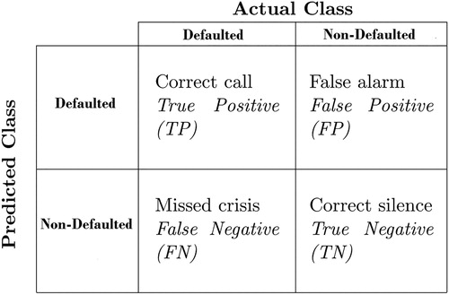
The calculation of the contingency matrix, under different threshold levels, can illustrate the performance capabilities of a binary classifier system. The receiver operating characteristic (ROC) curve plots the false positive rate (FPR) against the true positive rate (TPR), varying the threshold levels, as follows: [5] $$\mathit{FPR}=\frac{\mathit{FP}}{\mathit{FP}+\mathit{TN}}T\mathit{PR}=\frac{\mathit{TP}}{\mathit{TP}+\mathit{FN}}$$[5]

The precision recall (PR) curve instead plots the precision (P) versus the recall (R), varying the threshold levels, as follows: [6] $$P=\frac{\mathit{TP}}{\mathit{TP}+\mathit{FP}}R=\frac{\mathit{TP}}{\mathit{TP}+\mathit{FN}}$$[6]

While the previous measures take into account differences in the error types, further summaries can be calculated, such as the accuracy ratio. The accuracy of each model can be computed as: [7] $$\mathit{ACC}=\frac{\mathit{TP}+\mathit{TN}}{\mathit{TP}+\mathit{TN}+\mathit{FP}+\mathit{FN}}$$[7] and it characterizes the proportion of true results (both true positives and true negatives) among the total number of cases under examination.

Data

In this Section we describe the data set employed in our analysis and the necessary pre-processing stage.

We consider data supplied by Modefinance, a European Credit Assessment Institution (ECAI) that specializes in credit scoring for P2P platforms focused on SME commercial lending. Specifically, the analysis relies on a dataset composed of financial information (financial ratios calculated on balance sheets of the companies) on 9981 SMEs, mostly based in Southern Europe. Table 1 provides the summary statistics of the financial ratios contained in the original dataset obtained by modefinance.

Table 1. Summary statistics of the original dataset.

Statistic	N	Mean	St. Dev.	Min	Pctl (25)	Pctl (75)	Max
leverage_ratio	9,981	16.095	321.687	−5,249.217	1.111	10.568	25,798.100
total_asset_total_liab	9,981	2.137	27.787	0.002	1.057	1.532	2,598.092
current_ratio	9,981	4.381	207.257	0.001	0.959	1.796	20,514.310
quick_ratio	9,981	2.557	64.654	0.001	0.658	1.478	5,826.812
ROI	9,981	−7.012	195.250	−15,710.820	−0.405	3.528	472.135
ROE	9,981	7.119	462.523	−28,549.680	0.552	27.422	18,679.840
asset_turnover	9,981	1.303	1.540	−8.754	0.731	1.618	95.309
ROS	9,981	−35.312	1,652.441	−145,591.500	0.006	0.062	261.815
debt_coversion_ratio	9,981	39.608	5,382.764	−293,161.000	0.000	0.052	294,258.000
debt_ratio	9,981	0.995	5.597	0.0004	0.653	0.946	452.066
ROCE	9,981	12.998	1,099.395	−1,698.160	0.020	0.459	107,973.000

Note. For each balance sheet ratio we report the observed average (Mean) along with the standard deviation (St. Dev.), the minimum (Min), the 25-th and 75-th percentiles (Pctl) and the maximum (Max).

From Table 1 it is evident that the majority of the observed ratios show a presence of observations that lie at a large distance from the mean, which can be considered as outliers. Since a large presence of outliers can alter the results of regression models, we opt for removing data points greater than the 95th percentile and smaller than the 5th percentile. Table 2 provides the summary statistics of the resulting dataset.

Table 2. Summary statistics the transformed dataset.

Statistic	N	Mean	St. Dev.	Min	Pctl (25)	Pctl (75)	Max
leverage_ratio	7,033	8.475	10.482	−17.685	1.932	11.091	57.602
total_asset_total_liab	7,033	1.384	0.486	0.547	1.083	1.482	3.976
current_ratio	7,033	1.473	0.793	0.032	1.001	1.707	5.509
quick_ratio	7,033	1.157	0.745	0.002	0.686	1.379	4.970
ROI	7,033	1.600	4.799	−36.778	0.111	3.135	20.017
ROE	7,033	10.533	25.376	−103.360	0.802	19.717	142.834
asset_turnover	7,033	1.261	0.655	0.0001	0.790	1.603	4.043
ROS	7,033	0.035	0.062	−0.457	0.015	0.058	0.257
debt_coversion_ratio	7,033	0.103	0.386	−1.109	0.000	0.058	2.912
debt_ratio	7,033	0.784	0.189	0.251	0.675	0.924	1.830
ROCE	7,033	0.309	0.499	−1.729	0.059	0.414	2.934

Note. For each balance sheet ratio we report the observed average (Mean) along with the standard deviation (St. Dev.), the minimum (Min), the 25-th and 75-th percentiles (Pctl) and the maximum (Max).

From Table 2, note that most variables are on a similar scale. From a financial viewpoint, they represent different financial aspects of a company, as reported in the annual balance sheet, including information on the company financial exposure (leverage ratio, debt ratio), operational efficiency (ROI and ROE) and market power (asset turnover)

As a complementary note on the available data, we remark that many of the companies included in the sample are small and medium enterprises with less than 20 employees and a strong focus on manufacturing.

We finally point out that the proportion of companies in the sample that default in the year 2016 (one year after the reported financial information) is 2.9%, indicating a highly unbalanced sample, which makes statistical learning and predictive accuracy a quite challenging task.

Empirical findings

This Section is devoted to show the results of the analysis. First we report the similarity network obtained applying the methodology described in Section 2 to the data summarized in Table 2.

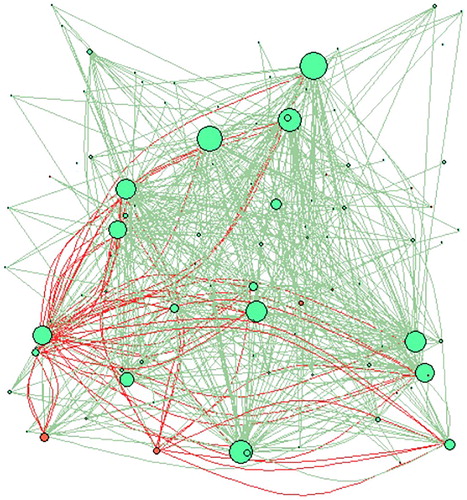
Figure 2 shows the minimal spanning tree representation of the borrowing companies network. Nodes are colored according to the financial soundness of the 7,033 considered companies, with red nodes representing defaulted companies and green nodes representing non-defaulted (active) ones.

Figure 2. Minimal spanning tree representation of the borrowing companies networks. The tree has been obtained by using the Euclidean distance between companies, based on the available 11 financial ratios institutions features and the Prim algorithm. Nodes are colored according to their financial soundness, red nodes represent defaulted institutions while green nodes are associated with active companies. Notice how defaulted institutions strongly occupy certain specific communities not being equally distributed among the networks.

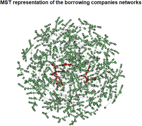
From Figure 2 note how defaulted institutions (marked in red) cluster with each other. This suggest that the topology of the network can be a relevant discriminator between different risk classes.

To better understand, and make more explainable, the network representation in Figure 2, we focus on three of the 11 considered financial variables: the asset turnover, indicating the market performance; the return on equity, indicating operational efficiency; and the leverage ration, indicating the level of financial sustainability of each company. All plots are based on the same sample, corresponding to about 10% of the considered companies.

Figure 3 shows the similarity network obtained using only the asset turnover to calculate correlations and, therefore, distances. In the figure, nodes are colored based on their status, with red indicating companies that have defaulted in the considered period, and green still active companies. The nodes are not equal but, rather, have a size proportional to their degree centrality, with bigger nodes indicating more connected ones. Edges are instead colored according to the sign of the found correlation: green for a positive correlation, and red for a negative correlation.

Figure 3. Correlation network based on the asset turnover.

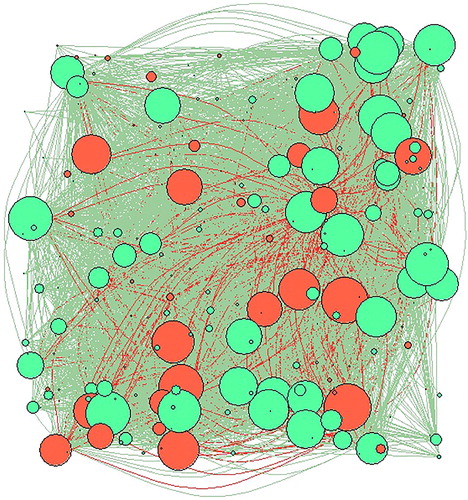
Figure 3 indicates that many companies are central and that, among them, there are both defaulted and not defaulted companies. This indicates the presence of a potential contagion effect, in terms of credit risk.

The graph also indicates that both negative and positive correlations arise. This indicates that the asset turnover ratio emphasizes mainly “similarities” between companies, expressed by positive edges, rather than dissimilarities, expressed by negative edges.

From an economic viewpoint, a positive edge between two companies indicates that their two relative sales volumes move together: they are complementary to each other so that when one fails the other is damaged too; a negative edge indicates instead that they are competing on the market so that, when one fails, the other gets the corresponding market share. The figure indicates that, in the considered data, complementarity prevails, and this reinforces the found presence of a contagion effect.

Figure 4 shows the network obtained using the leverage ratio to calculate correlations. The figure is based on the same assumptions as in Figure 3.

Figure 4. Correlation network based on the leverage.

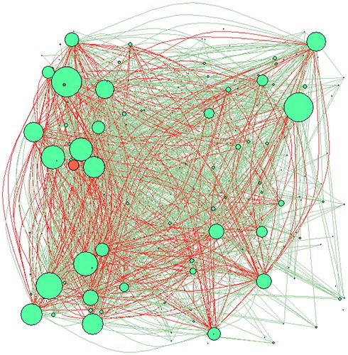
Figure 4 indicates that the central companies are much less than before and that most of them are good companies. In addition, the few that can be visualized appear to have a small centrality. This indicates a lower impact of contagion, through the leverage channel, than it was for the asset turnover. The finding can be an indication of the idiosyncratic nature of the leverage ratio, which leads to low correlations between defaulted and active companies. Conversely, what observed in Figure 3 for the asset turnover are high correlations between bad and good companies, which suggest the existence of a common systematic driver (such as the economic cycle), whose behavior induces correlations between all companies.

We also consider the similarity network model that emerges using the correlations between companies calculated in terms of the return on equity indicator over the considered period. Figure 5 presents the corresponding representation, maintaining the same assumptions as before.

Figure 5. Correlation network based on the return on equity. Number of nodes = 226.

Looking at Figure 5, the similarity network obtained using the return on equity indicator shows a low number of central nodes and a limited presence of defaulted companies. These findings point towards the idiosyncratic nature of the return on equity indicator, which appears company specific, rather than driven by a systematic driver, consistently with the economic intuition.

To summarize, the analysis of specific balance sheet ratios, that we retain representative of the main financial aspect of a company: market power (asset turnover), indebtness (leverage) and operational efficiency (ROE) reveal that the similarities in Figure 2 are most likely due to the companies sharing similar markets, rather than to their specific financial and/or operational management. This is indeed in line with the economic intuition, particularly in times of economic downturns as the considered one.

We now move to the calculation of the centrality measures, for the similarity network obtained in Figure 2.

Figure 6 shows the log-log plot of the cumulative distribution function and maximum likelihood power-law fit for the centrality measures employed in the analysis: degree, strength and PageRank. In the figure we separate the cumulative distributions of such measures, between the defaulted and the non-defaulted institutions.

Figure 6. Centrality measure distributions. The panels represent the distribution of the centrality measures separated according to the defaulted indicator γ, together with the corresponding power-law coefficient estimate. In the left panels, we represent the degree distributions, the central panels refer to the strength distributions while the right panels encompass the PageRank distributions. The different values of the scaling coefficients related to the distributions of defaulted and active institutions suggest their potential value for discriminating between such companies.

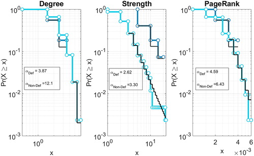
From Figure 6 note that, for all the considered centrality measures, we observe different scaling of the power-law exponents for institutions belonging to the defaulted set and for the sound ones. This suggests that the centrality measures that account for nodes’ importance are useful variables for discriminating between companies, and will likely improve credit scoring models.

To assess whether network centrality measures, embedded in network based scoring models, do improve standard models, we now compare the results obtained from different logistic regression models.

More precisely, Table 3 contains the estimates obtained applying three different types of logistic regression models: a logistic regression model with all explanatory variables; a logistic regression model with only the explanatory variables selected through a stepwise procedure (based on thresholding the deviance test p-value at 0.05); a logistic regression model with the variables selected by the previous stepwise procedure and the three considered centrality variables: degree, strength and page rank.

Table 3. Estimation results.

	Dependent variable
	Status
	(1)	(2)	(3)
leverage_ratio	−0.048*** (0.012)	−0.041*** (0.011)	0.001 (0.010)
total_asset_total_liab	0.943*** (0.358)	0.871** (0.358)	−0.767*(0.454)
current_ratio	−0.820** (0.322)	−0.802** (0.321)	−0.847*** (0.313)
quick_ratio	0.948*** (0.320)	0.934*** (0.320)	0.472 (0.330)
ROI	−0.011 (0.022)	−0.014 (0.020)	−0.014 (0.018)
ROE	−0.005* (0.003)
asset_turnover	−0.392** (0.166)	−0.427*** (0.165)	−0.620*** (0.162)
ROS	−6.792*** (1.359)	−7.032*** (1.326)	−0.675 (1.245)
debt_coversion_ratio	−0.049 (0.283)
debt_ratio	3.847*** (0.836)	3.467*** (0.835)	−0.573 (0.938)
ROCE	−0.012 (0.250)
degree_mst			−1.567*** (0.276)
strenght_mst			1.474*** (0.100)
pr_mst			−2,358.950 (5,601.062)
Constant	−6.933*** (1.122)	−6.573*** (1.128)	−0.457 (1.450)
Observations	4,924	4,924	4,924
Log Likelihood	−541.995	−543.455	−387.592
Akaike Inf. Crit.	1,107.991	1,104.911	799.184

Notes. (1) Logit regression with all variables; (2) Logit regression with stepwise selection of variables; (3) Logit regression with stepwise selection of variables and network parameters (estimated on the MST network).

*p < 0.1; **p < 0.05; ***p < 0.01.

From Table 3 note that in the regression output of Model (1) which includes all available financial ratios, eight variables are found statistically significant; most of them are in line with the expected sign of dependence. In particular, the asset turnover reports a negative sign, suggesting that companies stronger on the market are less likely to default. This is consistent with the results in Figure 3. This remains consistent across the two additional models we consider, that is, the step-wise selection and the network-augmented model. The estimated coefficient for the current ratio is highly statistically significant and has the expected negative sign, suggesting that companies with higher liquidity are less like to enter default. The debt and debt conversion ratios also report the expected sign and are found to be significant predictors of the SMEs’ probability of default. The leverage ratio reports an ambiguous sign for Model (1) and (2) whereas in the network-augmented specification, Model (3) is found not statistically significant. This consistently with what observed in Figure 4. Similar results are obtained for the ROE profitability indicator.

Looking at the network measures included in Model (3), we find both the degree and strength centrality to be statistically significant predictors of SMEs’ probability of default. In the context of the degree centrality, the finding indicates that the higher the number of connected companies, the lower the probability a company defaults. This is likely because it can “spread” its risk on more counterparts. On the other hand, the effect of the strength centrality counterbalances this effect, showing the presence of the complementarity contagion effect described before: companies with a high strength degree operate in complementary markets to many other companies and, therefore, are more affected by economic downturns, through contagion from the others.

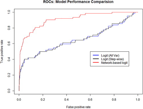
To compare the three models in terms of their predictive accuracy, Figure 6 reports the Receiver Operating Characteristic for all three models.

Figure 6 shows that the network based logistic regression model brings substantial improvement of the predictive performance. The AUROC of the three models are, respectively, equal to: 65.34, 65.39 and 90.89, showing a considerable improvement in predictive accuracy when network centralities are considered.

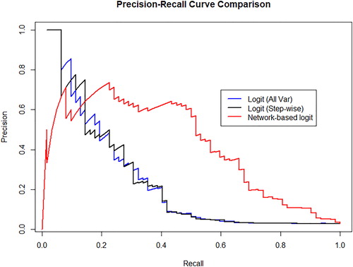
Figure 7 compares the models in terms of precision and recall.

Figure 7. Model comparison. The panels represent the comparison of the predictive performance of the three models considered taking into account the receiver operating characteristic curve for all three trained classifiers. Specifically, we represent the predictive performance of: (i) the logit classifier taking into account all available variables (black line), (ii) the logit classifier taking into account variables obtained through a stepwise selection and (iii) logit classifier taking into account variables obtained through a stepwise selection and the network parameters obtained from the MST representation of borrower companies.

Figure 8 shows once more the superior performance of the network based logistic regression model.

Figure 8. Precision Recall (PR) curves for the baseline credit risk models and for the network-augmented models. In the panel, similarly as in Figure 4, the blue line represents the precision-recall curve for the logit regression with all variables; the black line represents the precision-recall curve for the logistic regression with variables selected through step-wise and the red line represents the precision-recall for the network augmented regression.

The improvement in predictive performance determined by network models can also be appreciated looking at the predictions of the alternative models for 8 randomly selected companies in the test dataset, 4 known to be bad and 4 known to be good. The results are reported in Table 4.

Table 4. PD estimations of the three classifiers: (i) PD from baseline logit with all variables, (ii) PD from baseline logit with variables selected through step-wise, (iii) PD from network-augmented model.

Company	PD from BL	PD from BL (step)	PD from NAM	Status
Company A	0.171523	0.153451	0.895582	Defaulted
Company B	0.014322	0.01481	0.735145	Defaulted
Company C	0.116105	0.106103	0.887896	Defaulted
Company D	0.062864	0.058229	0.672447	Defaulted
Company E	0.014985	0.014741	0.008551	Active
Company F	0.447202	0.453344	0.263082	Active
Company G	0.327268	0.369632	0.131306	Active
Company H	0.471775	0.372646	0.098285	Active

From Table 4 note how the estimated PD of active companies decreases, moving from the baseline to the network based model. Conversely, the PD of defaulted companies increases moving along the same direction. This confirms, on real out-of-sample cases, the better predictive accuracy of the proposed network based models.

To summarize the results, it is quite clear that the inclusion of topological variables describing institutions centrality in similarity networks increases the predictive performance the credit scoring model. In addition, as our proposed model is, essentially, an augmented logistic regression model, its explainability remains high, differently to what occurs to many machine learning and deep learning models.

Besides the named advantages, our proposed model may have some drawbacks. First, the model is constrained by the simplified nature of similarity networks, which assume the adjacency matrix to be non-negative, thus inducing a mathematical asymmetry between positive and negative ties. The consequent summary measures, such as degree centrality, mean therefore something inherently different than in an unweighted network. To overcome this issue, more advanced network models could be considered, such as that of Labianca and Brass (2006), Stillman et al. (2017), Wilson et al. (2017) and Desmarais and Cranmer (2012). Second, logistic regression models may not be satisfactory in the presence of rare events or when more than one source of financial data is available. To overcome this issue, more advanced models can be employed, as shown in Giudici and Bilotta (2004), Figini and Giudici (2011), and Calabrese and Giudici (2015).

Conclusions

Peer-to-peer lending platforms, are becoming part of the everyday life. They can increase financial inclusion and user experience, but at the price of an increased credit risks, amplified by systemic risks, due to the high interconnectdness of Fintech platforms, which increases contagion.

Despite the fact that both classic banks and peer-to-peer platforms rely on credit scoring models for estimating credit risk, incentives for optimizing the model are different for peer-to-peer lending platforms since they, differently from banks, do not internalize credit risk that. Against this background, Fintech risk management becomes a central point of interest for regulators and supervisors, to protect consumers and preserve financial stability.

In this article we have shown how to exploit alternative data, generated by the platform themselves, to improve credit risk measurement. Specifically, we have shown how similarity networks can be exploited to increase the predictive performance of credit scoring models. To summarize the topological information contained in similarity networks we have calculated centrality measures and included them in logistic regression based scoring models. Our empirical results have revealed that the inclusion of centrality parameters can improve predictive accuracy. Furthermore, the obtained networks can be a very useful and “explainable” information of how risks are transmitted along an economic system.

The proposed network based credit scoring models can thus be usefully employed, not only by borrowers and lenders, to evaluate the performance of the platform, but also by regulators and supervisors to monitor peer to peer lenders, protecting consumers and safeguarding financial stability.

Acknowledgments

The authors thank the discussants, the participants and the organizers of Stu Hunter meeting in Villa Porro Poretti for a very stimulating research environment that has facilitated discussion and research improvements. The authors also thank the two anonymous referees, and the editor, for useful discussion and suggestions, which have led to an improved paper version.

Additional information

Funding

This research has received funding from the European Union’s Horizon 2020 research and innovation program “FIN-TECH: A Financial supervision and Technology compliance training programme” under the grant agreement No 825215 (Topic: ICT-35-2018, Type of action: CSA). In addition, the Authors thank ModeFinance, a European ECAI, for the data; the partners of the FIN-TECH European project, for useful comments and discussions.

References

- Ahelegbey, D. F., M. Billio, and R. Casarin. 2016. Bayesian graphical models for structural vector autoregressive processes. Journal of Applied Econometrics 31 (2):357. doi:10.1002/jae.2443.
- Allen, F., and D. Gale. 2000. Financial contagion. Journal of Political Economy 108 (1):1. doi:10.1086/262109.
- Barabasi, A. L. 2016. Network science. Cambridge University Press.
- Barrios, L. J. S., G. Andreeva, and J. Ansell. 2014. Monetary and relative scorecards to assess profits in consumer revolving credit. Journal of the Operational Research Society 65 (3):443–53. doi:10.1057/jors.2013.66.
- Battiston, S., D. Delli Gatti, M. Gallegati, B. Greenwald, and J. E. Stiglitz. 2012. Liasons dangereuses: Increasing connectivity risk sharing, and systemic risk. Journal of Economic Dynamics and Control 36 (8):1121. doi:10.1016/j.jedc.2012.04.001.
- Billio, M., M. Getmansky, A. W. Lo, and L. Pelizzon. 2012. Econometric measures of connectedness and systemic risk in the finance and insurance sectors. Journal of Financial Economics 104 (3):535. doi:10.1016/j.jfineco.2011.12.010.
- Bonacich, P. 2007. Some unique properties of eigenvector centrality. Social Networks 29 (4):555–64. doi:10.1016/j.socnet.2007.04.002.
- Brin, S., and L. Page. 1998. The anatomy of a large-scale hypertextual web search engine. Computer Networks and ISDN Systems 30 (1–7):107–17. doi:10.1016/S0169-7552(98)00110-X.
- Brunetti, C., J. H. Harris, S. Mankad, and G. Michailidis. 2015. Interconnectedness in the Interbank Market. FED Working Paper No 2015090.
- Calabrese, R., and P. S. Giudici. 2015. Estimating bank default with generalized extreme value regression models. Journal of the Operational Research Society 66 (11):1783–92. doi:10.1057/jors.2014.106.
- Claessens, S., J. Frost, G. Turner, and F. Zhu. 2018. Fintech credit markets around the world: Size, drivers and policy issues. Working Paper, Bank for International Settlements, Basel.
- Desmarais, B. A., and S. J. Cranmer. 2012. Statistical inference for valued-edge networks: The generalized exponential random graph model. PLoS One 7 (1):e30136. doi:10.1371/journal.pone.0030136.
- Emekter, R., Y. Tu, B. Jirasakuldech, and M. Lu. 2015. Evaluating credit risk and loan performance in online peer-to-peer (P2P) lending. Applied Economics 47 (1):54–70. doi:10.1080/00036846.2014.962222.
- Figini, S., and P. Giudici. 2011. Statistical merging of rating models. Journal of the Operational Research Society 62 (6):1067–74.
- Giudici, P., and A. Bilotta. 2004. Modelling operational loss: A Bayesian approach. Quality and Reliability Engineering International 20 (5):407–15. doi:10.1002/qre.655.
- Giudici, P., and B. Hadji-Misheva. 2017. P2P lending scoring models: Do they predict default? Journal of Digital Banking 2 (4):1–16.
- Giudici, P. S., and L. Parisi. 2018. CoRisk: Credit risk contagion with correlation network models. Risks 6 (3):95. doi:10.3390/risks6030095.
- Giudici, P. S., and A. Spelta. 2016. Graphical network models for international financial flows. Journal of Business and Economic Statistics 34 (1):126–38.
- Giudici, P. S., P. Sarlin, and A. Spelta. 2017. The interconnected nature of financial systems: Direct and common exposures. Journal of Banking and Finance. To Appear.
- Hautsch, N., J. Schaumburg, and M. Schienle. 2015. Financial network systemic risk contributions. Review of Finance 19 (2):685–738. doi:10.1093/rof/rfu010.
- Katz, L. 1953. A new status index derived from sociometric analysis. Psychometrika 18 (1):39–43. doi:10.1007/BF02289026.
- Kleinberg, J. M. 1999. Authoritative sources in a hyperlinked environment. Journal of the ACM 46 (5):604–32. doi:10.1145/324133.324140.
- Labianca, G., and G. Brass. 2006. Exploring the social ledger: Negative relationships and negative asymmetry. Academy of Management Review 31 (3):596–614. doi:10.5465/amr.2006.21318920.
- Lauritzen, S. L. 1996. Graphical models. Oxford: Clarendon Press.
- Leitner, Y. 2005. Financial networks: Contagion, commitment, and private sector bailouts. The Journal of Finance 60 (6):2925. doi:10.1111/j.1540-6261.2005.00821.x.
- Lorenz, J., S. Battiston, and F. Schweitzer. 2009. Systemic risk in a unifying framework for cascading processes on networks. The European Physical Journal B 71 (4):441–60. doi:10.1140/epjb/e2009-00347-4.
- Mantegna, R. N. 1999. Hierarchial structure in financial markets. The European Physical Journal B 11 (1):193–7. doi:10.1007/s100510050929.
- Milne, A., and P. Parboteeah. 2016. The business models and economics of peer-to-peer lending. Technical Report, European Credit Research Institute.
- Minoiu, C., and J. Reyes. 2010. A network analysis of global banking: 1978-2009. Washington, D.C.: IMF Working Paper, 11/74.
- Stillman, P. E., J. D. Wilson, M. J. Denny, B. A. Desmarais, S. Bhamidi, S. J. Cranmer, and Z. L. Lu. 2017. Statistical modeling of the default mode brain network reveals a segregated highway structure. Scientific Reports 7 (1):11694. doi:10.1038/s41598-017-09896-6.
- Wilson, J. D., M. J. Denny, S. Bhamidi, S. J. Cranmer, and B. A. Desmarais. 2017. Stochastic weighted graphs: Flexible model specification and simulation. Social Networks 49:37–47. doi:10.1016/j.socnet.2016.11.002.