A high dimensional functional time series approach to evolution outlier detection for grouped smart meters

Abstract

Smart metering infrastructures collect data almost continuously in the form of fine-grained long time series. These massive data series often have common daily patterns that are repeated between similar days or seasons and shared among grouped meters. Within this context, we propose an unsupervised method to highlight individuals with abnormal daily dependency patterns, which we term evolution outliers. To this end, we approach the problem from the standpoint of High Dimensional Functional Time Series and we use the concept of functional depth to exploit the dynamic group structure and isolate individual meters with a different evolution. The performance of the proposal is first evaluated empirically through a simulation exercise under different evolution scenarios. Subsequently, the importance and need for an evolution outlier detection method are shown by using actual smart-metering data corresponding to photo-voltaic energy generation and circuit voltage records. Here, our proposal detects outliers that might go unnoticed by other approaches of the literature that have demonstrated to be effective capturing magnitude and shape abnormalities.

Keywords:

• evolution outlier
• functional data
• functional depth
• functional time series
• high dimensional functional time series
• robustness
• smart meters
• unsupervised outlier detection

1. Introduction

Smart metering infrastructures are spreading and with them the ability to improve the quality, efficiency, and sustainability of electricity systems. Nowadays, numerous features such as energy consumption, household circuit voltage, and photo-voltaic energy generation are available for long time periods, at a very high-frequency rate. Furthermore, these features are contemporaneously collected for a multitude of grouped meters. For example, residential smart meters record data from different households in a given neighborhood or city (Street 2012). Another example is a solar energy farm collecting power generation data at the inverter level, providing as many time series as inverters (Kanal 2020). This data ecosystem provides not only big data but complex data structures that requires new advance methodologies (Meeker and Hong 2014; Sangalli 2018, 2020).

Within smart metering data analysis, outlier detection has become a topic of high interest (Sun et al. 2018). Additionally to its application to data quality (Angelos et al. 2011; Sun and Hou 2016; Jindal et al. 2016; Liu et al. 2020), outlier detection methods stand out due to their capability to monitor abnormalities and discover hidden patterns. Methodologies with this aim have been termed as outlier mining methods (Sun et al. 2018) and have been useful to reveal consumer behavior, capture energy theft, find system vulnerabilities and failures, and improve service quality (Angelos et al. 2011; Liu et al. 2020; Tanasa and Trousse 2004; Vallakati, Mukherjee, and Ranganathan 2015; Yin et al. 2019; Wang et al. 2019b).

The literature of outlier detection is vast and surveys on methodologies and applications have classified the literature by groups of data analytic methodologies (Sun et al. 2018; Blázquez-García et al. 2022; Himeur et al. 2021). Recently, Himeur et al. (2021) have provided an extensive taxonomy of the existing algorithms based on the different modules and parameters adopted, such as machine learning algorithms, feature extraction approaches, anomaly detection levels, computing platforms, and application scenarios. From the point of view of time series analysis, Blázquez-García et al. (2022) propose a classification by the type of input data (univariate or multivariate time series), outlier type (point, subsequence, or time series), and nature of the method (univariate or multivariate). Specific to the context of smart metering, Sun et al. (2018) classify the available approaches into distance-based methods, density-based methods, Support Vector Machines (SVM) methods and hybrid methods.

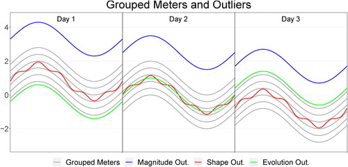
The above methodologies have been successfully used in many applications to detect abnormal phenomena of importance for smart meters problems. In fact, methods based on L-p distances between the observations of the meters’ functional feature of interest are particularly useful to identify magnitude outliers. For instance, the blue curve in Figure 1 represents an outlier of this kind since it is far away from the majority in all the days under consideration and, therefore, it features an abnormally large $\mathrm{L}-p$ distance with respect to the other curves. This figure also includes two other types of outliers. The red profile represents a shape outlier, since it is not far away from the majority, but it exhibits more wiggles than the other curves. The green one is an example of what we have termed an evolution outlier, because it has similar magnitude and shape as the majority, but its day-to-day variation is quite particular. Note that the green plot increases from day to day, while the other curves decrease. As a result, the green plot evolves abnormally with respect to its peers day after day. One important drawback of cross-sectional methods, like the ones based on L-p distances, is that they might fail to detect both shape outliers (Marron and Tsybakov 1995) and individuals evolving in time differently from the rest of the members of the group (i.e., what we have called evolution outliers).

Figure 1. Taxonomy of outliers. Magnitude (blue) and shape (red) outliers follow the decreasing dynamics from Day 1 to Day 3 of the bulk of data (grey curves). In contrast, the evolution outlier (green), which does not exhibit magnitude or shape differences, evolves differently than the grouped curves that share a decreasing day-to-day trend.

To overcome the difficulties in detecting shape outliers (like the red plot in Figure 1), the technical literature includes outlier detection methods based on Functional Data Analysis (FDA) (Ramsay and Silverman 2005; Ferraty and Vieu 2006; Srivastava and Klassen 2016; Dryden and Mardia 2016; Sangalli 2020). This branch of Statistics puts the focus on the morphological aspects of the observed curves, such as magnitude, shape, and derivatives, simplifying the task of outlier detection and the interpretation of the outcomes.

In this context of FDA, Arribas-Gil and Romo (2014) propose the Outliergram, which exploits the parabolic relationship between a functional depth measure and the Modified Epigraph Index (López-Pintado and Romo 2011) to identify shape outliers. Other authors approach the problem of shape outlier detection using the phase and amplitude decomposition of functional data (Marron et al. 2015; Srivastava and Klassen 2016; Dryden and Mardia 2016). In Xie et al. (2017) registration methods are used to separate the variability of functional data into amplitude and phase. Subsequently, each of these two components is visualized in boxplot-type plots, which allows for independent analysis and outlier detection for amplitude and phase. More recently, Harris et al. (2021) introduce the family of elastic depths, which are used with univariate boxplots and thresholding methods to improve the detection of abnormalities in shape. The authors use the elastic distances by Xie et al. (2017) to define amplitude and phase outlyingness measures that are converted into depths using the type-B construction of Zuo and Serfling (2000).

Yet, none of the available methods and approaches mentioned before are able to detect evolution outliers (like the green plot of Figure 1). Notice that this type of outlier only makes sense when dealing with samples of curves with temporal dependency, that is, with Functional Time Series (FTS) (Hörmann and Kokoszka 2012), and, more specifically, when dealing with a potentially very high number of FTS, as many as smart meters. Then, this outlier detection problem can be framed under the literature on High Dimensional Functional Time Series (HDFTS) (Gao, Shang, and Yang 2017, 2019). To the best of our knowledge, the plausibly daily outlying temporal evolution has been ignored so far when identifying potentially relevant outliers (Sun et al. 2018; Wang et al. 2019a). Only Raña, Aneiros, and Vilar (2015) proposed a bootstrap model-based method to detect periods of abnormal behavior, being only applicable to one single meter analysis. In this article, we aim at filling this gap by proposing a specific method to detect individual meters with abnormal evolution patterns from a group of meters with a common structure. Our proposal uses the information of functional depth measures (Tukey 1975; Gijbels and Nagy 2017) to exploit the group structure and isolate individual meters with a different evolution. These correspond to meters with abnormal inter-day evolution patterns or, in other words, individuals that do not follow the expected daily evolution mined from the group.

Additionally, we found that when the group of meters presents a common trend or periodical variation, the information contained in the functional depths might not be enough to capture evolution outliers with inverse behavior. For example, if the common trend is positive, our proposal based on functional depths could still miss evolution outliers with a negative trend. To overcome this drawback, we propose an enrichment of functional depth measures by incorporating the information of the Modified Epigraph Index.

Therefore, the main contributions of this work are:

• We propose a new class of abnormalities denoted as evolution outliers that are intrinsic to high-dimensional functional time series (HDFTS), under which smart meters data can be framed. Besides, we design an efficient evolution-outlier detection method to unmask meters with abnormal evolution patterns based on functional depth measures.

• We suggest a transformation of depth measures that empirically demonstrates to distinguish between increments and decrements produced by trends, and peaks and valleys produced by the time dynamics, so that these key features of the original smart meter time series are retained and are taken into account in the outlier detection procedure.

• We thoughtfully compare our proposal with several outlier detection methods, not only from the literature of Functional Data Analysis, but also with methods that have been successfully used in the literature of smart meters.

The rest of the article is organized as follows. Section 2 introduces the notation and definitions required to describe the methodology. Our evolution-outlier detection method is presented in Section 3. Then, in Section 4, we discuss results from a simulation study where we show the empirical superiority of our proposal against general-purpose methods of the literature to detect outliers. Additionally, we illustrate the use of the outlier detection methods with real case studies in Section 5. Finally, Section 6 draws some conclusions and outlines some avenues for further research.

2. Theoretical framework and definitions

2.1. From smart meter data to functional data

Let $\{\Gamma (u),u\in [1,p\times T]\}$ be one meter’s feature in the form of a time series that is recorded at p × T points during T windows (e.g., days) with a (daily) seasonality of length p. Then we consider each complete time series record as a discrete realization of the functional process, (1) $$y^t\left(x\right)=\left\{\Gamma \right(u),\hspace{1em}u=x+p(t-1\left)\right\},\hspace{1em}\hspace{1em}t\in 1,\dots ,T,\hspace{1em}1\le x\le p,$$(1) where t represents the index of windows (days) and $x\in [1,p]$ is the functions’ domain of definition.¹ In the context of smart meters, the domain is usually a range covering the twenty four hours of a day, typically from midnight to midnight. The result is a series of daily curves $\{y^1,\dots ,y^T\},$ that is, a Functional Time Series (FTS) (Hörmann and Kokoszka 2012). Importantly, modeling each sample as a curve allows us to take advantage of the functional nature of the data. This means, for example, that we can work with the first derivatives of the curves, which, as we illustrate in the case study of photo-voltaic energy generation of Section 5, can provide valuable information for outlier detection purposes.

Many meters provide many FTS, such as the one introduced in Eq. (1)(1) $$y^t\left(x\right)=\left\{\Gamma \right(u),\hspace{1em}u=x+p(t-1\left)\right\},\hspace{1em}\hspace{1em}t\in 1,\dots ,T,\hspace{1em}1\le x\le p,$$(1) . This data context can be framed into what is termed in the literature as a High Dimensional Functional Time Series (Gao, Shang, and Yang 2017, 2019), setup to which we stick in what follows. Given $i=1,\dots ,N$ being the index of the meters, a sample of high dimensional functions takes the following form: (2) $$\mathbf{y}=\left[\begin{array}{cccc}{y}_1^1& y_1^2& \dots & y_1^T\\ y_2^1& y_2^2& \dots & y_2^T\\ ⋮& ⋮& \ddots & ⋮\\ y_N^1& y_N^2& \dots & y_N^T\end{array}\right].$$(2)

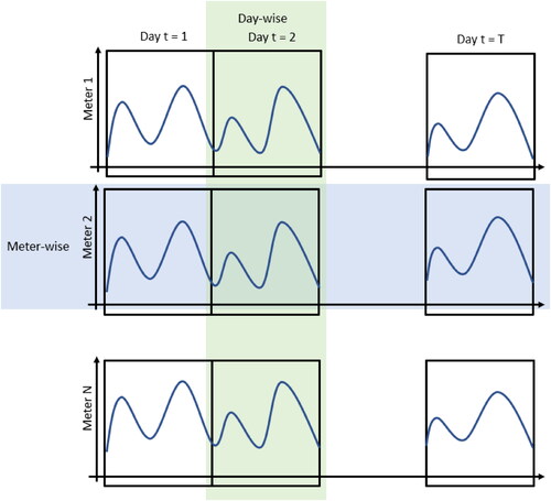
Figure 2 visualizes in a nutshell the information contained in the mathematical object y. Each row of Eq. (2)(2) $$\mathbf{y}=\left[\begin{array}{cccc}{y}_1^1& y_1^2& \dots & y_1^T\\ y_2^1& y_2^2& \dots & y_2^T\\ ⋮& ⋮& \ddots & ⋮\\ y_N^1& y_N^2& \dots & y_N^T\end{array}\right].$$(2) represents the information of one individual meter i (meter-wise), denoted by ${\mathbf{y}}_i^{*}.$ This is the FTS of $y_i^1,\dots ,y_i^T$ daily functions for one meter as in Eq. (1)(1) $$y^t\left(x\right)=\left\{\Gamma \right(u),\hspace{1em}u=x+p(t-1\left)\right\},\hspace{1em}\hspace{1em}t\in 1,\dots ,T,\hspace{1em}1\le x\le p,$$(1) . On the other hand, each column of Eq. (2)(2) $$\mathbf{y}=\left[\begin{array}{cccc}{y}_1^1& y_1^2& \dots & y_1^T\\ y_2^1& y_2^2& \dots & y_2^T\\ ⋮& ⋮& \ddots & ⋮\\ y_N^1& y_N^2& \dots & y_N^T\end{array}\right].$$(2) represents the information of a single day t (day-wise), denoted by ${\mathbf{y}}_{*}^t.$ This is a sample of N daily functions $y_1^t,\dots ,y_N^t$ where each one represents a meter for the same day. In the following, to ease notation, we denote by $y^1,\dots ,y^T$ the sample of T functions for a given meter (meter-wise) and by $y_1,\dots ,y_N$ the sample of N functions for a given day (day-wise).

Figure 2. Context—Data from multiple smart meters.

2.2. Functional depth measures

The estimation of well-known statistics such as the median and quantiles are based on the ability to rank or order a data sample. An important property of these statistics based on rankings is that they have the ability to be insensitive to extreme observations or, in other words, they are robust. This fact has made them fundamental tools to construct outlier detection methods such as the classical Boxplot (Tukey 1975). However, the notion of order is only unique and straightforward in the univariate case.

To provide a notion of ordering for multivariate and high dimensional spaces, the literature has proposed the concept of depth measures (Tukey 1975; Zuo and Serfling 2000; Gijbels and Nagy 2017). More concretely, in this article, we are interested in functional depths, which provide an ordering of a sample of curves and, in consequence, functional order statistics counterparts as the functional median. There are many different definitions of functional depths, which, according to Nagy et al. (2016), can be divided in general into two main families, namely, integrated and nonintegrated ones. The first class is defined by taking integrals over given collections of depths of low-dimensional projections of functions (Fraiman and Muniz 2001; López-Pintado and Romo 2011). In contrast, the nonintegrated ones replace the integral by the infimum or supremum of these low-dimensional projections (Mosler 2013; Narisetty and Nair 2016). Other authors have proposed functional depths particularly tailored to take into account shape features of the curves (Harris et al. 2021) based on alignment methods, which allow to separate phase and amplitude variability (Marron et al. 2015; Srivastava and Klassen 2016). Here, we opt for the family of integrated depths because they feature clear practical advantages to cope with smart meters data (Sun et al. 2018; Wang et al. 2019a), namely: Fast computation of the empirical version of the integrated functional depth and its theoretical guarantees Nagy et al. (2016), given the massive amount of data smart metering systems might contain (Sun, Genton, and Nychka 2012); availability of integrated depths that do not require preprocessing (smoothing or alignment); and availability of integrated depths that can deal with missing data or set of curves observed on different domains (Elías et al. 2022).

Formally, let FD be a general integrated functional depth. This statistic evaluates the centrality of a given function y from a sample of functions $y^1,\dots ,y^T$ with respect to the center of symmetry of its empirical distribution P_T. This empirical distribution belongs to a functional random variable taking values in a space of continuous functions defined in a domain $[1,p].$ For $x\in [1,p],$ we denote as $P_{T,x}$ the marginal distribution of P_T at slice x and its cumulative marginal distribution as $F_{T,x}.$ In practice, functional data is observed as a set of discrete points or evaluations of the curves. To simplify the exposition, we assume that the points in the grid at which the curves are observed/evaluated are common for all the functions and equal to $\tilde{x}=1,2,\dots ,p.$ However, as we said above, there are partially observed integrated functional depths applicable when the collection of discretized points varies from curve to curve without the need of preprocessing (Elías et al. 2022). Then, the empirical integrated functional depth is defined as (3) $$\text{FD}(y,P_T)=\sum _{\tilde{x}=1}^{p}w(\tilde{x})·\mathrm{D}(y(\tilde{x}),P_{T,\tilde{x}}),$$(3) being $w(\tilde{x})$ a weighting function that sums up to 1, and D a suitable depth. More specifically, according to Zuo and Serfling (2000), a depth function $\mathrm{D}$ should be affine invariant, maximal at the center, monotone with respect to the deepest point, and should vanish at infinity. In the same vein, Nagy et al. (2016) and Gijbels and Nagy (2017) study, adapt and complete the counterparts of these properties for functional depths.

In essence, Eq. (3)(3) $$\text{FD}(y,P_T)=\sum _{\tilde{x}=1}^{p}w(\tilde{x})·\mathrm{D}(y(\tilde{x}),P_{T,\tilde{x}}),$$(3) assigns a real number to each y, typically between 0 and 1. The highest value is the deepest function, whereas lower values correspond to observations that are outliers with respect to the sample of functions. Let us denote by $y^{[1]},\dots ,y^{[T]}$ the center-outward ordering, being $y^{[1]}$ the deepest function, and $y^{[T]}$ the most outlying curve of the sample. The statistic $y^{[1]}$ is a natural functional analog of the median and the literature has considered it as a robust estimator of the center of the distribution of the functions.

Different functions D provide different integrated functional depths. For example, let us consider the well-known Modified Band Depth (López-Pintado and Romo 2009), which is defined by (4) $$\text{MBD}(y,P_T)=\frac{1}{p}\sum _{\tilde{x}=1}^{p}2F_{T,\tilde{x}}\left(y\right(\tilde{x}\left)\right)(1-F_{T,\tilde{x}}(y\left(\tilde{x}\right)\left)\right).$$(4)

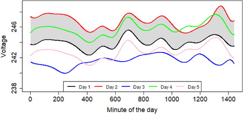
The MBD is built by plugging $w(\tilde{x})=1/p$ and $\mathrm{D}\left(y\right(\tilde{x}),P_{T,\tilde{x}})=2F_{T,\tilde{x}}\left(y\right(\tilde{x}\left)\right)(1-F_{T,\tilde{x}}(y\left(\tilde{x}\right)\left)\right)$ in Eq. (3)(3) $$\text{FD}(y,P_T)=\sum _{\tilde{x}=1}^{p}w(\tilde{x})·\mathrm{D}(y(\tilde{x}),P_{T,\tilde{x}}),$$(3) . In plain words, MBD accounts for the average time that a given function lies inside all the possible bands built with pairs of the sample curves. As an illustration, Figure 3 shows a synthetic row sample (see meter-wise in Figure 2) of smart meters data, that is, 5 days of voltage circuit values for one household, meaning that there are $(\begin{array}{c}T\\ 2\end{array})=(\begin{array}{c}5\\ 2\end{array})=10$ possible bands. One of these bands is represented using the functions Day 1 and Day 2 (grey region). Day 4 is inside that band for a high proportion of the minutes of the day, whereas Day 3 and Day 5 are completely outside. Following this reasoning, notice that Day 1 is completely inside all the possible bands, thus achieving the highest depth value. In contrast, Day 2 and Day 3 have the two smallest depth values.

Figure 3. Synthetic voltage example for one meter for 5 days.

Finally, Eq. (3)(3) $$\text{FD}(y,P_T)=\sum _{\tilde{x}=1}^{p}w(\tilde{x})·\mathrm{D}(y(\tilde{x}),P_{T,\tilde{x}}),$$(3) allows introducing the Modified Epigraph Index (MEI) (López-Pintado and Romo 2011), which is used in outlier detection methods, although it is not a functional depth. It measures the mean proportion of curves lying above a given function y and is defined as (5) $$\text{MEI}(y,P_T)=\frac{1}{p}\sum _{\tilde{x}=1}^p(1-F_{T,\tilde{x}}(y(\tilde{x}))).$$(5)

It is straightforward to see that MEI is obtained by replacing $\mathrm{D}(y(\tilde{x}),P_{T,\tilde{x}})$ by $1-F_{T,\tilde{x}}(y(\tilde{x}))$ and $w(\tilde{x})=1/p$ in Eq. (3)(3) $$\text{FD}(y,P_T)=\sum _{\tilde{x}=1}^{p}w(\tilde{x})·\mathrm{D}(y(\tilde{x}),P_{T,\tilde{x}}),$$(3) . Continuing with the example of Figure 3, Day 3 is the one with the highest MEI since it has a high proportion of curves (4 out of 5) above it almost all the time. In contrast, Day 2 has the smallest MEI. In Section 3, we leverage this statistic to provide a meaningful and useful modification of functional depths to detect evolution outliers.

3. Methodology for evolution-outlier detection

Our idea is to exploit functional depth measures to capture the dynamic daily evolution of smart meter data. With this goal in mind, we use the FTS provided by each meter i, that is, each row of the object y of Eq. (2)(2) $$\mathbf{y}=\left[\begin{array}{cccc}{y}_1^1& y_1^2& \dots & y_1^T\\ y_2^1& y_2^2& \dots & y_2^T\\ ⋮& ⋮& \ddots & ⋮\\ y_N^1& y_N^2& \dots & y_N^T\end{array}\right].$$(2) denoted as ${\mathbf{y}}_i^{*}$ (meter-wise in Figure 2). This is T daily functions for each single meter, and we compute the depth values of each of the functions in the sample of curves ${\mathbf{y}}_i^{*}=\{y^1,\dots ,y^T\}.$ That is, for each $t=1,\dots ,T,$ we obtain $\text{FD}(y^t,{\mathbf{y}}_i^{*}).$ Hereafter, we denote $\text{FD}(y^t,{\mathbf{y}}_i^{*}),$ as $\text{FD}(t),$ that is, the functional depth value of the day t with respect to its historical records. Then, our approach is focused on the analysis of these depths arranged as the following time series $$\{\text{FD}(t),\hspace{1em}t\in (1,\dots ,T)\}.$$

To illustrate the intuition behind our proposal, see Figure 4. The top-left panel shows a FTS that increases in magnitude from t = 1 to t = 5 or, in other words, it has a positive trend component. The deepest function is the green curve, t = 3, and the curves with the smallest depth values are the red and the black curves, t = 1 and t = 5. The top-central panel arranges depth values as a time series $\text{FD}(t)$ where each point is related to one curve. Then, the highest depth is observed at time point t = 3 and the two lowest are observed at t = 1 and t = 5. On the other hand, the bottom-left panel illustrates the same FTS but with a decreasing trend component. That is, we invert the time order of the curves: see, for example, the position of the blue curve in the top and bottom left panels. The time depths $\text{FD}(t)$ for this FTS with inverse trend is represented again in the central bottom panel, featuring exactly the same pattern as that of the FTS on the top panel.

Figure 4. Time series of FD and time series of scaled FD for two Functional Time Series.

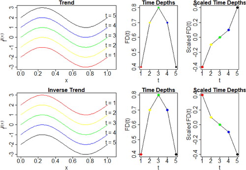
This toy example illustrates how depth measures are able to track the time position of each curve and how the corresponding time series of depths retain characteristics of the FTS. However, time series of depths only account for the relative position of a function with respect to the center and do not discriminate between deviations above or below the central deepest function. So, two functions with the same depth value might be in opposite locations with respect to the center (see that the FD values of the green and blue curves are the same in both the top and bottom panels). As illustrated above, the FTS in the top panel of Figure 4 and the inverted FTS emphasize this problem; curves in yellow, red, black and blue have a different overall position with respect to the center, some are above and the others below. Nevertheless, the depth values are not able to capture this feature.

To overcome this drawback, we incorporate the information provided by the Modified Epigraph Index (MEI) to depth measures. Using this statistic, introduced in Eq. (5)(5) $$\text{MEI}(y,P_T)=\frac{1}{p}\sum _{\tilde{x}=1}^p(1-F_{T,\tilde{x}}(y(\tilde{x}))).$$(5) , we define what we call the scaled depth as (6) $$\text{SFD}(y)=\mathit{sgn}(\text{MEI}(y^{\left[1\right]})-\text{MEI}(y))$$(6) (7) $$\times (\text{FD}(y^{\left[1\right]})-\text{FD}(y)),$$(7) where sgn stands for the sign function and $y^{[1]}$ is the functional median. The term (6) takes into account whether or not a function is above or below the median curve, being positive if it is above and negative otherwise. On the other hand, term (7) centers the $\text{SFD}$ in zero, being this value associated with the deepest curve. Now, functions below the median have a negative $\text{SFD},$ while these are positive for functions above the median. We remark that our aim is not to provide a new definition of depth, but we scale the depth to retain the sign of temporal trends and seasons. In fact, it is easy to see that the scaled depth is not a depth, for example, it does not satisfy properties P-2 (maximality at the center) and P-3 (monotonically decrease with respect to the deepest point) (Nagy et al. 2016; Gijbels and Nagy 2017). About P-2, the scaled depth achieves its maximum at 1 and this value is not the center of symmetry, which is zero. Regarding P-3, the center is zero and its value might increase or decrease if the functions move far from the center upwards or downwards.

Analogously to depth measures, the scaled depth measures provide a time series where each of the time points represents the value of a given day t, $$\{\text{SFD}(t),\hspace{1em}t\in (1,\dots ,T)\}.$$

The time series of scaled depth is defined to capture the trend and seasonal patterns of the original time series. This is illustrated in the right-hand panels of Figure 4 where the scaled depth measures are plotted. Now, the information of the positive and negative trends are retained in the scaled depths. This is visually evident by an increasing and decreasing time series of scaled depths.

Given N meters, we thus have ${\text{FD}}_i(t)$ and ${\text{SFD}}_i(t)$ for $i=1,\dots N.$ For simplicity, we continue the exposition for ${\text{SFD}}_i(t)$ but everything can be extrapolated to ${\text{FD}}_i(t).$ These N time series of ${\text{SFD}}_i(t)$ are gathered in the following multivariate time series of scaled depths, (8) $$\mathbf{SFD}(t)=[{\text{SFD}}_1(t),{\text{SFD}}_2(t),\dots ,{\text{SFD}}_N(t)].$$(8)

Daily dependent data must result in time series in Eq. (8)(8) $$\mathbf{SFD}(t)=[{\text{SFD}}_1(t),{\text{SFD}}_2(t),\dots ,{\text{SFD}}_N(t)].$$(8) that vary in a structured way. Additionally, since we are focusing on meters that belong to a group, this multivariate time series must be synchronized sharing common movements among meters. Hence, deviations from this common evolution would determine an abnormal dependency pattern. Notice that evolution outlying meters might result in outlying time series ${\text{SFD}}_i(t)$ that could bias the estimation of the mean evolution. For this reason, to obtain an unbiased estimator of the common evolution, we use the trimmed mean of $\mathbf{SFD}(t)$ (Fraiman and Muniz 2001) as a robust estimator of the overall time dependency pattern captured by scaled depths. This is (9) $$\mu \text{SFD}(t)=\frac{1}{\lceil N/2\rceil }\sum _{r=1}^{\lceil N/2\rceil }{\text{SFD}}_{\left[r\right]}(t),$$(9) being ${\text{SFD}}_{[r]}(t)$ the r-th time series of $\mathbf{SFD}(t)$ with the highest depth. Intuitively, Eq. (9)(9) $$\mu \text{SFD}(t)=\frac{1}{\lceil N/2\rceil }\sum _{r=1}^{\lceil N/2\rceil }{\text{SFD}}_{\left[r\right]}(t),$$(9) computes the mean at each time point t but only considering the fifty percent of the most central time series. In other words, it removes the fifty per cent of the most atypical time series $\text{SFD}(t)$ for the computation of the mean. We term $\mu \text{SFD}(t)$ as “baseline” since it is a reference of the common evolution captured by depth or scaled depth.

Then, we use the Euclidean distance between each time series in $\mathbf{SFD}(t)$ and the baseline $\mu \text{SFD}(t)$ to find individuals with a time evolution that is far from the baseline evolution, that is, $$\text{dist}({\text{SFD}}_i(t),\mu \text{SFD}(t))=\sqrt{\sum _{t=1}^T({\text{SFD}}_i(t)-\mu \text{SFD}(t){)}^2}.$$

Large values of $\text{dist}(·,\mu \text{SFD}(t))$ indicate that the dependency pattern is abnormal with respect to the baseline evolution.

The next step is to define a threshold or cutoff to determine which element from the vector of distances d is large enough to be unmasked as an evolution outlier. To avoid any distributional assumption, we opt for the flexible adaptation of the classical Tukey’s Boxplot rule by Hubert and Vandervieren (2008). It includes a robust measure of skewness and a correction term in the determination of the whiskers. More precisely, we highlight a given meter i as an outlier if its distance with respect to the baseline exceeds the right whisker, that is, $$\text{dist}\left({\text{SFD}}_i\right(t),\mu \text{SFD}(t\left)\right)>Q_3\left(\mathbf{d}\right)+\gamma \times {\hspace{0.17em}\exp \hspace{0.17em}}^{3MC}\times \mathit{IQR}\left(\mathbf{d}\right),$$ where Q₃ and IQR are the third quantile and the interquartile range, MC the medcouple statistics, ${\hspace{0.17em}\exp \hspace{0.17em}}^{3MC}$ the exponential correction model suggested by Hubert and Vandervieren (2008), and γ a parameter to tune the length of the whiskers. Hubert and Vandervieren (2008) set it to 1.5 to leave roughly 1% of probability in both tails but, since we are only looking for right-tailed outliers, we consider $\gamma =0.72$ to leave approximately 5% only in the right tail of the distribution. Note that the flexibility of this rule comes from the fact that, if the distribution of d is symmetric (MC = 0), the proposal by Hubert and Vandervieren (2008) turns out to be the classical Tukey’s Boxplot. Therefore, it only corrects under departures from the symmetry assumption.

In summary, the methodology includes the steps described in Algorithm 1. We use the short name “TDEPTH” to refer to the methodology based on the application of Algorithm 1 to the time series of functional depths computed as in Eq. (3)(3) $$\text{FD}(y,P_T)=\sum _{\tilde{x}=1}^{p}w(\tilde{x})·\mathrm{D}(y(\tilde{x}),P_{T,\tilde{x}}),$$(3) , while “STDEPTH” alludes to the scaled depth that we have defined in Eqs. (6)(6) $$\text{SFD}(y)=\mathit{sgn}(\text{MEI}(y^{\left[1\right]})-\text{MEI}(y))$$(6) and (7)(7) $$\times (\text{FD}(y^{\left[1\right]})-\text{FD}(y)),$$(7) . Both of these methods can be applied to the data curves themselves and their derivatives, as we do in the numerical experiments of Section 5.

Algorithm 1:

Evolution outlier detection method

Input: Data and parameter γ

Output: Evolution outlier status of i

1 for i $\stackrel{}{\leftarrow }$ 1 to N do

2 Compute the time series SFD ${}_i(t)$

3 end

4 Compute the baseline evolution μSFD(t)

5 for i $\stackrel{}{\leftarrow }$ 1 to N do

6 Compute the distance d_i between SFD ${}_i(t)$ and μSFD(t)

7 end

8 Compute $c=Q_3(\mathbf{d})+\gamma \times {\hspace{0.17em}\exp \hspace{0.17em}}^{3MC}\times \mathit{IQR}(\mathbf{d})$

9 for i $\stackrel{}{\leftarrow }$ 1 to N do

10 if ${\mathrm{d}}_i$ > c then

11 i is an outlier

12 else

13 i is not an outlier

14 end

15 end

4. Results on synthetic data sets

4.1. Simulation setup

The simulation setting is based on two parts. The first one aims to generate a set of non-atypical meters with a common evolution structure (group effect) and individual variations to each meter (meter effect). The second part consists in generating evolution outliers by modifying the group effect and/or the meter effect components. In the following, we propose two different models: The first one demonstrates the ability of our proposal to detect evolution outliers by comparison against general-purpose outlier identification methods available in the technical literature. The second one shows why it is important to reformulate the standard notion of functional depth to detect some particular types of evolution outliers.

Model 1: This model generates a common evolution pattern for the non-outlier individuals and produces evolution outliers by adding a temporal trend. We simulate a sample of N typical meters with T daily curves as follows: (Group mean) $$y_i^t(x)=\hspace{0.17em}\sin \hspace{0.17em}(2\pi x)+$$(Group mean) (Group effect) $${ϵ}^t(x)+$$(Group effect) (Meter effect) $${\upsilon }_i(x),$$(Meter effect) being ${ϵ}^t(x)$ and ${\upsilon }_i(x)$ zero-mean Gaussian processes with covariance functions $Co{v}_{ϵ}(x,x\prime )={\eta }_{ϵ}{e}^{-{\lambda }_{ϵ}|x-x\prime |}$ and $Co{v}_{\upsilon }(x,x\prime )={\eta }_{\upsilon }{e}^{-{\lambda }_{\upsilon }|x-x\prime |},$ respectively (Rasmussen and Williams 2005). The parameters were set to ${\eta }_{ϵ}=0.8,{\lambda }_{ϵ}={\lambda }_{\upsilon }=0.1$ and ${\eta }_{\upsilon }=1.5.$

To generate a meter i that behaves as an evolution outlier, we select a starting time point for the trend, t_a, from $t\in 1,\dots ,T-\rho$ and an end point, t_b, so that the trend remains during ρ periods. Then, the trend is generated as a functional linear interpolation between the curve $y_i^{t_a}$ and the curve $y_i^{t_b}.$ More precisely, $$y_{\text{Out}1}^t(x)=\{\begin{array}{cc}\frac{t_b-t}{t_b-t_a}{y}_i^{t_a}(x)+\frac{t-t_a}{t_b-t_a}{y}_i^{t_b}(x)\hfill & \text{for}\mathrm{ }t\in t_a,\dots ,t_b,\hfill \\ y_i^t(x)\hfill & \text{otherwise}.\hfill \end{array}$$

For these outliers, we fix ${\eta }_{\upsilon }=0.5.$

Model 2: This model generates a group of meters with a common trend and includes evolution outliers by inverting the sign of the trend. We simulate a sample of N typical meters with T daily curves as follows: (Group mean) $$y_i^t(x)=\hspace{0.17em}\sin \hspace{0.17em}(2\pi x)+$$(Group mean) (Group trend) $$\frac{T-t}{T-1}{ϵ}^1(x)+\frac{t-1}{T-1}{ϵ}^T(x)+$$(Group trend) (Meter effect) $${\upsilon }_i(x),$$(Meter effect)

The parameters were set to ${\eta }_{ϵ}=0.8$ and ${\lambda }_{ϵ}=0.1$ for the group trend and ${\eta }_{\upsilon }=1.5$ for the meter effect. The model above includes a common trend that is increasing or decreasing depending on the difference between ${ϵ}^1$ and ϵ^T.

To generate an outlier with an opposite trend we revert the pattern as follows (Group mean) $$y_{\text{Out}2}^t(x)=\hspace{0.17em}\sin \hspace{0.17em}(2\pi x)+$$(Group mean) (Outlying trend) $$\frac{t-1}{T-1}{ϵ}^1(x)+\frac{T-t}{T-1}{ϵ}^T(x)+$$(Outlying trend) (Meter effect) $${\upsilon }_i(x).$$(Meter effect)

4.2. Benchmark methods

Benchmark methods are chosen to cover the taxonomy of classes proposed by the survey of outliers detection methods for smart meters (Sun et al. 2018). Additionally, we include large-scale unusual time series detection (Hyndman, Wang, and Laptev 2015) and FDA methods (Arribas-Gil and Romo 2014; Sun and Genton 2011; Xie et al. 2017; Harris et al. 2021). To apply FDA methods in our context of High Dimensional Functional Time Series, we compute the outliers for each row of Eq. (2)(2) $$\mathbf{y}=\left[\begin{array}{cccc}{y}_1^1& y_1^2& \dots & y_1^T\\ y_2^1& y_2^2& \dots & y_2^T\\ ⋮& ⋮& \ddots & ⋮\\ y_N^1& y_N^2& \dots & y_N^T\end{array}\right].$$(2) (day-wise) and, then, we identify a meter as abnormal if it has been detected as an outlier more than a given percentage of the days under analysis. For our proposals, TDEPTH and STDEPTH, we consider the Modified Band Depth (MBD) (López-Pintado and Romo 2009), Fraiman and Muniz Depth (FMD) (Fraiman and Muniz 2001), Extremal Depth (EXTD), (Narisetty and Nair 2016) and Infimal Depth (INFD) (Mosler 2013). The list of final methods and their implementation are:

• Distance-based methods: K-Nearest Neighbors (KNN) (Ramaswamy, Rastogi, and Shim 2000) and Aggregate KNN (AKNN) (Angiulli and Pizzuti 2002). To set the parameter K we try a range of values and we show the results of the best performance. Given the KNN and the AKNN scores, we determine as outlier those individuals with scores larger than $Q3+1.5*\mathit{IQR}.$

• Local density methods: Local Outlier Factor (LOF) (Breunig et al. 2000), Connectivity Based Outlier Factor (COF) (Tang et al. 2002) and Influenced Local Outlier Factor (INFLO) (Jin et al. 2006). Since these methods depend on the K-Nearest Neighbors, we follow the same procedure as with the distance-based methods to select the parameter K and the outlier detection rule.

• One-class classification (ONESVM): We perform one-class Support Vector Machines (Schölkopf et al. 1999) classification with radial and polynomial kernels. The parameter of the radial kernel was fixed to 0.05. We show the results of the best performing kernel.

• Time series feature selection (FEA): Following (Hyndman, Wang, and Laptev 2015), we compute, for each meter, several time series indicators such as auto-covariance features, entropy, lumpiness, flat spots, crossing points, mean, variance, maximum level shift and maximum variance shift. Then, we apply Principal Components Analysis to the data set of the features and we detect outliers in the reduced two-dimensional space produced by the first two principal components. As outlier detection methods, SVM with radial or polynomial kernel and the $\alpha -$ hull method are considered. We show the results of the best performing method among SVM and $\alpha -$ hull.

• Dimension reduction methods (PCA): We apply Principal Components Analysis to our original data set and apply one-class SVM classification to the reduced two-dimensional space. We show the results of the best performing method among SVM and $\alpha -$ hull.

• Functional Boxplot (FBOX): We apply the functional Boxplot by Sun and Genton (2011) day-wise with the MBD and with its default parameters for the whiskers.

• Outliergram (OUTGRAM): We apply the functional Outliergram by Arribas-Gil and Romo (2014) day-wise with the default parameters for the lower bound parabola.

• Geometric Boxplot (GEOM): We apply the method for shape outlier detection by Xie et al. (2017) day-wise to detect amplitude abnormalities (AMP) and phase abnormalities (PHASE).

• Elastic Depth Boxplot (ELASTIC): Also with a focus on shape outliers, Harris et al. (2021) propose a definition of elastic depth and provide an algorithm to detect outliers in terms of amplitude (AMP) and phase (PHASE).

4.3. Performance metrics

To measure the performance of the outlier detection methods, we compute the True Positive Rate (TPR) and the True Negative Rate (TNR) (Gaur et al. 2019), which are: $$\begin{array}{l}\text{TPR}=\frac{\#\text{True}\mathrm{ }\text{Detected}\mathrm{ }\text{Outliers}}{\#\text{Outliers}},\\ \text{TNR}=\frac{\#\text{True}\mathrm{ }\text{Detected}\mathrm{ }\text{No}\mathrm{ }\text{Outliers}}{\#\text{No}\mathrm{ }\text{outliers}}.\end{array}$$

TPR (sensitivity) measures the fraction of anomalous events identified by a method and TNR (specificity) measures the fraction of non-anomalous events identified by the method. Therefore, the best performance would be provided by a method with $\text{TPR}=\text{TNR}=1.$ In contrast, a method that is not useful to detect the outliers at all would provide $\text{TPR}=0$ and $\text{TNR}=1.$

4.4. Results

We generate samples with N = 100 and T = 50. Besides the N meters, we add a 1%, 5% and 10% of outliers. Then, we report the mean values of TPR and TNR for 100 replicates of this experiment. These values are collated in Tables 1 and 2 for each of the two data-generating models described in Subsection 4.1.

Table 1. Simulation results for Model 1.

Outliers		1%		5%		10%
		TPR	TNR	TPR	TNR	TPR	TNR
KNN		0.000	0.899	0.010	0.903	0.014	0.900
AKNN		0.000	0.930	0.000	0.9316	0.003	0.924
LOF		0.250	0.884	0.198	0.8914	0.197	0.892
COF		0.180	0.950	0.102	0.9477	0.092	0.961
INFLO		0.240	0.961	0.194	0.960	0.181	0.963
ONESVM		0.510	0.582	0.392	0.5772	0.398	0.590
FEA		0.450	0.506	0.522	0.5083	0.248	0.478
PCA		0.450	0.506	0.522	0.5083	0.248	0.478
TDEPTH
	MBD	1.000	1.000	1.000	1.000	1.000	1.000
	FMD	1.000	1.000	1.000	1.000	1.000	1.000
	EXTD	1.000	1.000	1.000	1.000	1.000	1.000
	INFD	1.000	0.936	1.000	0.978	1.000	0.987
STDEPTH
	MBD	1.000	1.000	1.000	1.000	1.000	1.000
	FMD	1.000	1.000	1.000	1.000	1.000	1.000
	EXTD	1.000	1.000	1.000	1.000	1.000	1.000
	INFD	1.000	0.950	1.000	0.976	1.000	0.986
FBOX		0.000	0.988	0.000	0.986	0.000	0.986
OUTGRAM		0.000	0.953	0.000	0.952	0.005	0.943
GEOM
	AMP	0.000	1.000	0.000	1.000	0.000	1.000
	PHASE	0.000	1.000	0.000	1.000	0.000	1.000
ELASTIC
	AMP	0.000	1.000	0.000	1.000	0.000	1.000
	PHASE	0.000	1.000	0.000	1.000	0.000	1.000

Table 2. Simulation results for Model 2.

Outliers		1%		5%		10%
		TPR	TNR	TPR	TNR	TPR	TNR
KNN		0.490	0.9015	0.388	0.916	0.371	0.920
AKNN		0.140	0.931	0.072	0.941	0.086	0.944
LOF		0.620	0.889	0.678	0.904	0.571	0.920
COF		0.580	0.956	0.608	0.960	0.446	0.9711
INFLO		0.520	0.962	0.130	0.961	0.051	0.961
ONESVM		0.310	0.721	0.548	0.694	0.551	0.698
FEA		0.540	0.506	0.460	0.504	0.602	0.514
PCA		0.540	0.506	0.460	0.504	0.602	0.514
TDEPTH
	MBD	0.000	1.000	0.000	1.000	0.000	1.000
	FMD	0.000	1.000	0.000	1.000	0.000	1.000
	EXTD	0.000	1.000	0.000	1.000	0.000	1.000
	INFD	0.250	0.9455	0.222	0.9532	0.158	0.960
STDEPTH
	MBD	1.000	1.000	1.000	1.000	0.980	1.000
	FMD	1.000	1.000	1.000	1.000	0.980	1.000
	EXTD	1.000	1.000	1.000	1.000	0.980	1.000
	INFD	1.000	0.968	1.000	0.9747	0.980	0.989
FBOX		0.020	0.991	0.014	0.9904	0.009	0.992
OUTGRAM		0.040	0.953	0.04	0.959	0.031	0.959
GEOM
	AMP	0.000	1.000	0.000	1.000	0.000	1.000
	PHASE	0.000	1.000	0.000	1.000	0.000	1.000
ELASTIC
	AMP	0.000	1.000	0.000	1.000	0.000	1.000
	PHASE	0.000	1.000	0.000	1.000	0.000	1.000

Table 1 shows the results of Model 1 (ρ = 5) and, in bold numbers, we highlight the best performing method. These are the proposed outlier detection methods TDEPTH and STDEPTH, which tie, both having $\text{TPR}=\text{TNR}=1$ for all the functional depths considered, except for INFD, which achieves TNR values slightly lower than 1. They are followed by local-density methods (LOF, COF and INFLO) but with $\text{TPR}$ values far away from 1. The results of distance-based (KNN and AKNN) and functional data methods (FBOX and OUTGRAM) show that, as expected, they do not have capability of detecting these evolution outliers. Finally, FEA and PCA seem to split the individuals into two random groups given the values of TPR and TNR around 0.5. To show how the methods perform when there are not outliers, we have re-run the simulation of Model 1 with the same parameters but without outliers (results not included in the article). As expected, the methods that were unable to detect outliers behave similarly and get a TNR equal to 1. In contrast, the methods that were able to detect some outliers achieve a value slightly smaller than 1 but our proposals are never smaller than 0.95. For example, the worst performing method among all the evolution outlier proposals in 100 replicates was STDEPTH MBD and it achieved a mean TNR 0.95 with a standard deviation of 0.03.

The results of Model 2 are shown in Table 2. As expected, TDEPTH does not perform well in these circumstances as motivated in Section 2. However, our scaled proposal, STDEPTH, achieves values for $\text{TPR}$ and $\text{TNR}$ that are again close to one, meaning that it is still able to capture this particular evolution abnormality. The second best performing method for Model 2 is LOF that improves with respect Model 1 but they are still far from the results provided by STDEPTH.

In addition to the gains in performance, we found that the methods based on integrated or non integrated depths (i.e., FMD, MBD, EXTD, and INFD) are by far faster than the ones based on Elastic distances or depths. The mean computational cost involved in one replica of our simulation is 26 hours for ELASTIC, based on the elastic depth, and 11 hours for GEOM. In contrast, MBD takes 9.36 seconds and EXTD 2.86 seconds.

In conclusion, the results in Tables 1 and 2 clearly demonstrate that, among all existing outlier detection techniques in the technical literature, our methodology is the only one able to efficiently capture these evolution outliers, aside from being computationally tractable in real big data contexts. In the next section, we corroborate the usefulness and importance of our approach by identifying evolution outliers that remain undetected by other methods on real data of household voltage circuit and solar energy generation.

5. Results on real data sets

Next we use the advocated FDA approach to evolution outlier detection with real smart meter data. Additionally, to cover the complete taxonomy of outliers introduced in Figure 1, we also apply the functional Boxplot (Sun and Genton 2011) and the Outliergram (Arribas-Gil and Romo 2014), two of the most efficient methods to detect magnitude and shape outliers in a manageable computational time. Specifically, we use the Pecan Street data set (Street 2012) that provides access to 1-minute records of smart meters from Austin over one year. We use freely available data of voltage circuit (25 households) and solar energy generation (19 households²).

In all the results, the parameters are set with their default values as explained in Section 3. Additionally, for photo-voltaic data, we work with the non-zero solar generation profiles, obviating night time periods. The FDA methods are applied to the smoothed level data and the first derivatives. To smooth the data and to estimate the derivatives, we use cubic B-splines and the number of basis functions K is selected to minimize the mean squared error (Ramsay and Silverman 2005; Ferraty and Vieu 2006).

Table 3 shows the identifiers of the households that have been detected as magnitude outliers (M), shape outliers (S) or evolution outliers (E and $\tilde{\mathrm{E}}$ stand for time series of depths and time series of scaled depths, respectively). Columns 2-5 include the outliers detected using the level data, while columns 6-9 report those found by using the first derivative. In what follows, we remark on the key learnings.

Table 3. Identifiers of the detected Magnitude (M), Shape (S), Evolution based on depth (E) and Evolution based on scaled depth ($\tilde{\mathbf{E}}$) outliers.

		Zero derivative					First derivative
	Meter id	M	S	E	$\tilde{\mathbf{E}}$		M	S	E	$\tilde{\mathbf{E}}$
Voltage	vol5746			✓			✓
	vol6139			✓			✓
	vol7901			✓	✓		✓
	vol9019			✓
	vol9922						✓
	vol7951						✓
Solar	sol9019								✓
	sol6139								✓
	sol3538									✓

Evolution outliers are not detected by other depths: As Table 3 shows, the methodology proposed in this article allows us to uncover outliers that are not caught by existing methods for detecting magnitude or shape functional outliers. In particular, although meter vol₉₀₁₉ is not identified as a magnitude or shape outlier, this household follows an abnormal daily voltage evolution with respect to the group of households and therefore, it is classified as an evolution outlier. Figure 5a shows 305 daily curves for a non-outlier household (vol₂₈₁₈) and Figure 5b the corresponding daily curves for the detected evolution outlier (vol₉₀₁₉). Each daily curve is colored with a rainbow palette (Hyndman and Shang 2010) associated with the calendar day, that is, similar colors are days which are close in time.

Figure 5. Voltage circuit: evolution outlier not detected with other method. (a) Non-outlier vol2818. (b) Outlier vol9019. (c) Time series of depths.

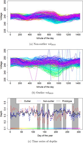
A preliminary visual inspection of Figure 5a and b reveals the outlying nature of vol₉₀₁₉ in comparison with vol₂₈₁₈. They show that voltage daily curves of the same period of time have a different relative magnitude position for the non-outlier and for the outlier. However, one should expect roughly synchronized evolution for two households fed by the same substation branch. Specifically, the outlier profile has a group of green curves located in low values of voltage, while they are located centrally for the non-outlier. Light blue curves are above the majority for the outlier household; and for the non-outlier, they are located below and in the middle of the majority of the curves.

The difference in the evolution is more evident in Figure 5c where the time series of depths, $\text{FD}(t),$ are represented for the non-outlier and the outlier. Moreover, the baseline, $\mu \text{FD}(t),$ is plotted with a solid line. Here, the outlier (dotted line) moves far away from the baseline, while, in contrast, the non-outlier (dashed line) remains close to it.

First derivatives allow detecting those outliers not detected with level data: Another remark from Table 3 is that the use of the first derivatives discloses outliers not unmasked with the functions’ values themselves. This is the case for the circuit voltage of the outlying households vol₉₉₂₂ and vol₇₉₅₁, which are two of the just six households that do not have photo-voltaic energy generation. The effect of not having solar energy generation on the household circuit voltage is not large enough to be caught with level data, however, the derivatives intensify the shape differences and they are detected as outliers in the magnitude of the derivative.

Similarly, the first derivatives allow highlighting households with abnormalities in terms of solar energy generation. While magnitudes of solar profiles are determined by the amount of power generation installed, the shapes are highly influenced by the panels orientation and tilt. In fact, the two households sol₆₁₃₉ and sol₉₀₁₉, which are detected as evolution outliers (E) in the first derivatives, have their solar panels set to the south, whereas the majority of the households are south-west-oriented.³

For a better understanding of these evolution outliers, Figure 6a shows the time series of depths of one outlier household (sol₆₁₃₉), one non-outlier household (sol₄₇₆₇) and the baseline. The time series of depths for the non-outlier and the outlier are not far from the baseline, meaning that their daily evolution is fairly similar. In contrast, if we consider the first derivatives, more discrepancies appear. To see this, Figure 6b represents the time depths of the same households and the baseline computed on the first derivatives where the outlier profile is farther from the baseline than the non-outlier (shaded grey regions).

Figure 6. Photo-voltaic energy generation: Computed depths on the derivatives allow detecting outliers not unmasked by the analysis without derivatives. (a) Time series of depths computed on the zero derivative. (b) Time series of depths computed on the first derivative.

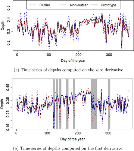
This points to the fact that the analysis of the derivatives might capture the shape differences in the daily generation solar profile due to the differences of panel orientation and tilt. Therefore, our methodology can be useful, for example, to detect outliers in terms of panel settings when data of a group of meters with a similar panel configuration are available.

Scaled depths unmask those outliers which are not detected with regular depths: A household with a systematic growth of voltage, for example, would provide time depths that are similar to a household whose voltage circuit systematically decreases. In contrast, scaled depths are especially defined to shed light on differences in these variations in trends and seasons. Table 3 shows that the use of scaled depths ($\tilde{\mathrm{E}}$) with photo-voltaic solar energy generation captures the household sol₃₅₃₈ as an outlier whereas it is not captured with the other methods, including classical depths.

Figure 7 illustrates this particular case. More precisely, Figure 7a shows the regular time depths of the outlier household (sol₃₅₃₈) and one non-atypical (sol₄₇₆₇) computed on the first derivatives of solar energy generation. Both time series of depths are close to the baseline. However, the scaled depths $\text{SFD}$ represented in Figure 7b highlight periods where the atypical is remarkably far from the baseline (shaded grey regions).

Figure 7. Photo-voltaic energy generation: Scaled depths detect outliers not detected by classical depths. (a) Time series of depths. (b) Time series of scaled depths.

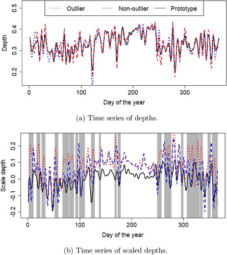
Additionally, we see that the $\text{SFD}$ of the outlier is generally above the baseline when the differences with the baseline are large. This means that the solar setting of this household provides a daily profile with larger periods of growth (positive derivatives) than the majority of the households, especially at the start and end of the year. In fact, checking the Pecan Street metadata, sol₃₅₃₈ is the third largest solar installation facing west and the smallest facing south. This setting produces a double-humped daily profile with a maximum peak of generation that occurs later in the day than that of the majority.

6. Conclusion

To fill the absence of methodologies focused on temporal daily dependency for smart meters data (Sun et al. 2018; Wang et al. 2019a), we propose an outlier detection method that is able to uncover evolution outliers that remain undetected by current methods. The underlying methodology takes advantage of the analysis of multiple grouped meters to extract joint information that affects them equally. The methodology is based on the concept of functional depth (Zuo and Serfling 2000; Gijbels and Nagy 2017) and, among all the available definitions in the literature, we suggest to use the family of integrated functional depths and its versions for partially observed functional data (Nagy et al. 2016; Elías et al. 2022), because of their practical advantages to cope with some of the main challenges posed by smart meters data (Sun et al. 2018; Wang et al. 2019a). Additionally, when the evolution outlier arises from a difference in the sign of trends or seasons, we propose a scaled version that empirically demonstrates its superiority against the original definition. However, the scaled version might suffer when the number of curves and/or the number of observed points per curve is small.

Our empirical results show that our proposal outperforms other benchmark methods not only in terms of outlier detection but also in terms of computational efficiency. Furthermore, the pitfalls of not taking into account the time dimension in the task of outlier mining has been shown with actual smart meters data of voltage circuit and solar energy generation. Using voltage circuit, our proposal captures evolution abnormalities that remain hidden with other methods that are specifically tailored for magnitude and shape outliers. In this context, our approach for grouped meters captures deviations from common dynamics of households fed by the same substation that should have roughly synchronized evolution patterns. On the other hand, the temporal evolution plays an important role in the analysis of solar energy generation. Here, only the application of our functional approach to the first derivatives allows highlighting abnormalities due to the differences of panel orientation and tilt. This feature makes our approach an appealing method to monitor solar farms with a given panel configuration or solar tracker systems.

In summary, our outlier detection method proposal, in conjunction with the available methods from the literature, covers a wide and general class of possible atypical phenomena, namely, shape, magnitude, and evolution outliers. This classification might support in the crucial tasks of monitoring, understanding the sources of the potential abnormality and supporting the decision to intervene. Future research lines will include the study of the statistical properties of the scaled depth as well as the theoretical relationship between the time series of depths and the time dynamics of different classical Functional Time Series models.

Acknowledgements

The authors are grateful for insightful comments and suggestions from two reviewers. The authors thankfully acknowledge the computer resources, technical expertise, and assistance provided by the SCBI (Supercomputing and Bioinformatics) center of the University of Málaga.

Additional information

Funding

This work was supported in part by the Spanish Ministry of Science and Innovation through project PID2020-115460GB-I00, and in part by the Andalusian Regional Government through project P20-00153, and in part by the Research Program for Young Talented Reseachers of the University of Málaga under Project B1-2020-15. This project has also received funding from the European Social Fund and the European Research Council (ERC) under the European Union’s Horizon 2020 research and innovation program (grant agreement No. 755705).

Notes on contributors

A. Elías

Antonio Elías received the Economics Degree in 2013, and his PhD degree in Statistics in 2020 from Carlos III University of Madrid, Madrid, Spain. He currently holds a post-doctoral position with the Department of Applied Mathematics, University of Malaga. His research interest include functional data analysis, non-parametric statistics, time series analysis and outlier detection.

J. M. Morales

Juan Miguel Morales received the Industrial Engineering degree from the University Malaga, Malaga, Spain, in 2006, and his PhD degree in electrical engineering from the University of Castilla-La Mancha, Ciudad Real, Spain, in 2010. He is currently an Associate Professor with the Department of Applied Mathematics, University of Malaga. His research interests include power systems economics, operations and planning, energy analytics and optimization, smart grids, decision-making under uncertainty, and electricity markets.

S. Pineda

Salvador Pineda received the Industrial Engineering degree from the University of Malaga, Malaga, Spain, in 2006, and his PhD degree in electrical engineering from the University of Castilla-La Mancha, Ciudad Real, Spain, in 2011. He is currently an Associate Professor with the Department of Electrical Engineering, University of Malaga. His research interests include power system operation and planning, electricity markets, renewable integration, energy policy, game theory, and optimization.

Notes

1 Note that in Eq. (1)(1) $$y^t\left(x\right)=\left\{\Gamma \right(u),\hspace{1em}u=x+p(t-1\left)\right\},\hspace{1em}\hspace{1em}t\in 1,\dots ,T,\hspace{1em}1\le x\le p,$$(1) the functions’ domain are defined as $x\in [1,p],$ that is, as a continuous interval. Therefore, the points at which the observed curves are evaluated need not to be equally spaced but simply bounded between the extreme values of that interval.

2 Given the metadata of the Pecan Street data set, households 8,565, 8,386, 9,922, 5,746, 7,951 and 7,901 do not have photo-voltaic energy generation.

3 Panel tilt is not available from the metadata of the Pecan Street data set to have the complete picture of the solar panel setting.

References

- Angelos, E. W. S., O. R. Saavedra, O. A. C. Cortés, and A. N. de Souza. 2011. Detection and identification of abnormalities in customer consumptions in power distribution systems. IEEE Transactions on Power Delivery 26 (4):2436–42. doi: 10.1109/TPWRD.2011.2161621.
- Angiulli, F., and C. Pizzuti. 2002. Fast outlier detection in high dimensional spaces. In Principles of data mining and knowledge discovery, ed. T. Elomaa, H. Mannila, and H. Toivonen, 15–27. Berlin, Heidelberg: Springer Berlin Heidelberg.
- Arribas-Gil, A., and J. Romo. 2014. Shape outlier detection and visualization for functional data: The outliergram. Biostatistics (Oxford, England) 15 (4):603–19. doi: 10.1093/biostatistics/kxu006.
- Blázquez-García, A., A. Conde, U. Mori, and J. A. Lozano. 2022. A review on outlier/anomaly detection in time series data. ACM Computing Surveys 54 (3):1–33. doi: 10.1145/3444690.
- Breunig, M. M., H.-P. Kriegel, R. T. Ng, and J. Sander. 2000. LOF: identifying density-based local outliers. ACM SIGMOD Record 29 (2):93–104. doi: 10.1145/335191.335388.
- Dryden, I. L., and K. V. Mardia. 2016. Statistical shape analysis, with applications in R. 2nd ed. Wiley Series in Probability and Statistics. Chichester: John Wiley and Sons.
- Elías, A., R. Jiménez, A. M. Paganoni, and L. M. Sangalli. 2022. Integrated depths for partially observed functional data. Journal of Computational and Graphical Statistics 1–12. doi: 10.1080/10618600.2022.2070171.
- Ferraty, F., and P. Vieu. 2006. Nonparametric functional data analysis: Theory and practice. New York: Springer-Verlag.
- Fraiman, R., and G. Muniz. 2001. Trimmed means for functional data. Test 10 (2):419–40. doi: 10.1007/BF02595706.
- Gao, Y., H. L. Shang, and Y. Yang. 2017. High-dimensional functional time series forecasting. In Functional statistics and related fields, ed. G. Aneiros, E. G. Bongiorno, R. Cao, and P. Vieu, 131–6. Cham: Springer International Publishing.
- Gao, Y., H. L. Shang, and Y. Yang. 2019. High-dimensional functional time series forecasting: An application to age-specific mortality rates. Journal of Multivariate Analysis 170:232–43 (Special Issue on Functional Data Analysis and Related Topics). doi: 10.1016/j.jmva.2018.10.003.
- Gaur, M., S. Makonin, I. V. Bajić, and A. Majumdar. 2019. Performance evaluation of techniques for identifying abnormal energy consumption in buildings. IEEE Access 7:62721–33. doi: 10.1109/ACCESS.2019.2915641.
- Gijbels, I., and S. Nagy. 2017. On a general definition of depth for functional data. Statistical Science 32 (4):630–9. doi: 10.1214/17-STS625.
- Harris, T., J. D. Tucker, B. Li, and L. Shand. 2021. Elastic depths for detecting shape anomalies in functional data. Technometrics 63 (4):466–76. doi: 10.1080/00401706.2020.1811156.
- Himeur, Y., K. Ghanem, A. Alsalemi, F. Bensaali, and A. Amira. 2021. Artificial intelligence based anomaly detection of energy consumption in buildings: A review, current trends and new perspectives.” Applied Energy 287:116601.
- Hörmann, S., and P. P. Kokoszka. 2012. Functional time series: Handbook of statistics, Vol. 30, 157–86. Netherlands: Elsevier B.V.
- Hubert, M., and E. Vandervieren. 2008. An adjusted boxplot for skewed distributions. Computational Statistics & Data Analysis 52 (12):5186–201. doi: 10.1016/j.csda.2007.11.008.
- Hyndman, R. J., and H. L. Shang. 2010. Rainbow plots, bagplots, and boxplots for functional data. Journal of Computational and Graphical Statistics 19 (1):29–45. doi: 10.1198/jcgs.2009.08158.
- Hyndman, R. J., E. Wang, and N. Laptev. 2015. Large-scale unusual time series detection. In 2015 IEEE International Conference on Data Mining Workshop (ICDMW), Atlantic City, NJ, USA, November 14, pp. 1616–9.
- Jin, W., A. K. H. Tung, J. Han, and W. Wang. 2006. Ranking outliers using symmetric neighborhood relationship. In Advances in knowledge discovery and data mining, ed. W.-K. Ng, M. Kitsuregawa, J. Li, and K. Chang, 577–93. Berlin, Heidelberg: Springer Berlin Heidelberg.
- Jindal, A., A. Dua, K. Kaur, M. Singh, N. Kumar, and S. Mishra. 2016. Decision tree and SVM-based data analytics for theft detection in smart grid. IEEE Transactions on Industrial Informatics 12 (3):1005–16. doi: 10.1109/TII.2016.2543145.
- Kanal, A. 2020. Kaggle: Solar power generation data. https://www.kaggle.com/anikannal/solar-power-generation-data/metadata (accessed March 26, 2021).
- Liu, S., Y. Liang, J. Wang, T. Jiang, W. Sun, and Y. Rui. 2020. Identification of stealing electricity based on big data analysis. 2020 The 7th International Conference on Power and Energy Systems Engineering. Energy Reports 6:731–8. doi: 10.1016/j.egyr.2020.11.138.
- López-Pintado, S., and J. Romo. 2009. On the concept of depth for functional data. Journal of the American Statistical Association 104 (486):718–34. doi: 10.1198/jasa.2009.0108.
- López-Pintado, S., and J. Romo. 2011. A half-region depth for functional data. Computational Statistics & Data Analysis 55 (4):1679–95. doi: 10.1016/j.csda.2010.10.024.
- Marron, J. S., J. O. Ramsay, L. M. Sangalli, and A. Srivastava. 2015. Functional data analysis of amplitude and phase variation. Statistical Science 30 (4):468–84. http://www.jstor.org/stable/24780816.
- Marron, J. S., and A. B. Tsybakov. 1995. Visual error criteria for qualitative smoothing. Journal of the American Statistical Association 90 (430):499–507. doi: 10.1080/01621459.1995.10476541.
- Meeker, W. Q., and Y. Hong. 2014. Reliability meets big data: Opportunities and challenges. Quality Engineering 26 (1):102–16. doi: 10.1080/08982112.2014.846119.
- Mosler, K. 2013. Depth statistics. In Robustness and complex data structures, ed. G. Biau, 17–34. Heidelberg: Springer.
- Nagy, S., I. Gijbels, M. Omelka, and D. Hlubinka. 2016. Integrated depth for functional data: Statistical properties and consistency. ESAIM. Probability and Statistics 20:95–130.
- Narisetty, N. N., and V. N. Nair. 2016. Extremal depth for functional data and applications. Journal of the American Statistical Association 111 (516):1705–14. doi: 10.1080/01621459.2015.1110033.
- Ramaswamy, S., R. Rastogi, and K. Shim. 2000. Efficient algorithms for mining outliers from large data sets. ACM SIGMOD Record 29 (2):427–38. doi: 10.1145/335191.335437.
- Ramsay, J. O., and B. W. Silverman. 2005. Functional data analysis. Springer Series in Statistics. Berlin: Springer.
- Rasmussen, C. E., and C. K. I. Williams. 2005. Gaussian processes for machine learning. Cambridge, MA: MIT Press. doi: 10.7551/mitpress/3206.001.0001.
- Raña, P., G. Aneiros, and J. M. Vilar. 2015. Detection of outliers in functional time series. Environmetrics 26 (3):178–91. doi: 10.1002/env.2327.
- Sangalli, L. M. 2018. The role of statistics in the era of big data. Statistics & Probability Letters 136:1–3. https://www.sciencedirect.com/science/article/pii/S016771521830155X.
- Sangalli, L. M. 2020. A novel approach to the analysis of spatial and functional data over complex domains. Quality Engineering 32 (2):181–90. doi: 10.1080/08982112.2019.1659357.
- Schölkopf, B., R. Williamson, A. Smola, J. Shawe-Taylor, and J. Platt. 1999. Support vector method for novelty detection. In Proceedings of the 12th International Conference on Neural Information Processing Systems, NIPS’99, 582–8. Cambridge, MA, USA: MIT Press.
- Srivastava, A., and E. P. Klassen. 2016. Functional and shape data analysis. New York, NY: Springer.
- Street, P. 2012. Real energy. Real constumers. In real time. http://www.pecanstreet.org/energy/.
- Sun, L., K. Zhou, X. Zhang, and S. Yang. 2018. Outlier data treatment methods toward smart grid applications. IEEE Access 6:39849–59. doi: 10.1109/ACCESS.2018.2852759.
- Sun, W., and J. Hou. 2016. A MPRM-based approach for fault diagnosis against outliers. Neurocomputing 190:147–54. doi: 10.1016/j.neucom.2016.01.023.
- Sun, Y., and M. G. Genton. 2011. Functional boxplots. Journal of Computational and Graphical Statistics 20 (2):316–34. doi: 10.1198/jcgs.2011.09224.
- Sun, Y., M. G. Genton, and D. C. Nychka. 2012. Exact fast computation of band depth for large functional datasets: How quickly can one million curves be ranked? Stat 1 (1):68–74. doi: 10.1002/sta4.8.
- Tanasa, D., and B. Trousse. 2004. Advanced data preprocessing for intersites Web usage mining. IEEE Intelligent Systems 19 (2):59–65. doi: 10.1109/MIS.2004.1274912.
- Tang, J., Z. Chen, A. Wai-Chee Fu, and D. W. Cheung. 2002. Enhancing effectiveness of outlier detections for low density patterns. In Advances in knowledge discovery and data mining, ed. M.-S. Chen, P. S. Yu, and B. Liu, 535–48. Berlin, Heidelberg: Springer Berlin Heidelberg.
- Tukey, J. W. 1975. Mathematics and the picturing of data. In Proceedings of the International Congress of Mathematics, Vancouver, 1974, Vol. 2, 523–31.
- Vallakati, R., A. Mukherjee, and P. Ranganathan. 2015. A density based clustering scheme for situational awareness in a smart-grid. In 2015 IEEE International Conference on Electro/Information Technology (EIT), Dekalb, IL, USA, pp. 346–50.
- Wang, Y., Q. Chen, T. Hong, and C. Kang. 2019a. Review of smart meter data analytics: Applications, methodologies, and challenges. IEEE Transactions on Smart Grid 10 (3):3125–48. doi: 10.1109/TSG.2018.2818167.
- Wang, Z., G. Li, X. Wang, C. Chen, and H. Long. 2019b. Analysis of 10kV non-technical loss detection with data-driven approaches. In 2019 IEEE Innovative Smart Grid Technologies – Asia (ISGT Asia), Chengdu, China, pp. 4154–8. doi: 10.1109/ISGT-Asia.2019.8881733.
- Xie, W., S. Kurtek, K. Bharath, and Y. Sun. 2017. A geometric approach to visualization of variability in functional data. Journal of the American Statistical Association 112 (519):979–93. doi: 10.1080/01621459.2016.1256813.
- Yin, T., S. S. Wulff, J. W. Pierre, and T. J. Robinson. 2019. A case study on the use of data mining for detecting and classifying abnormal power system modal behaviors. Quality Engineering 31 (2):314–33. doi: 10.1080/08982112.2018.1530356.
- Zuo, Y., and R. Serfling. 2000. General notions of statistical depth function. The Annals of Statistics 28 (2):461–82. http://www.jstor.org/stable/2674037.