Monitoring univariate processes using control charts: Some practical issues and advice

Abstract

We provide an overview and discussion of some issues and guidelines related to monitoring univariate processes with control charts. We offer some advice to practitioners to help them set up control charts appropriately and use them most effectively. We propose a four-phase framework for control chart set-up, implementation, use, and maintenance. In addition, our recommendations may be useful for researchers in the field of statistical process monitoring. We identify some current best practices, some misconceptions, and some practical issues that rely on practitioner judgment.

Keywords:

• average run length
• control chart
• rational subgrouping
• statistical process monitoring

1. Introduction

Control charts are used for monitoring variables of interest to support the quality management of goods and services. First introduced by Shewhart (1931) to distinguish between expected (or common cause) variation and variation due to assignable causes, control charts are applied in a wide variety of industries and in healthcare applications.

With a control chart one plots over time the statistics related to key variables that reflect the quality of a process or product. In the simplest case, if the value of the control chart statistic falls within the control chart limits, the process is considered in control, and any observed variation is considered common cause variation. Conversely, if a value of the control chart statistic exceeds the control limits, there is an indication of a potential process change that may need attention. In this case, the observed variation in the process or product is potentially due to a removable assignable cause. Control charts are used to understand variation over time with the goal of process improvement. Process improvement in industrial applications is typically characterized by centering the process on a specified target value and reducing variation.

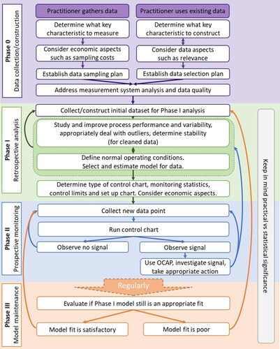
In our view process monitoring consists of the following four phases: Phase 0, Phase I, Phase II, and Phase III, where most of the discussion in the statistical process monitoring (SPM) literature has been devoted to Phase I and II issues. It seems that the terms Phase I and Phase II were first used by Alt et al. (1976), although the ideas go back much further. In our view, we also need a Phase 0, terminology first suggested by Megahed, Wells, and Camelio (2010) and discussed in Megahed and Jones-Farmer (2015), Megahed (2019), and Lamooki et al. (2021), for data collection, and a Phase III for model and chart maintenance.

In Phase 0, the steps depend on whether the data is gathered for the monitoring purpose or whether an existing data source will be used. When data will be gathered, it should be determined what key characteristics should be measured and how they should be measured, thereby accounting for economic aspects such as sampling costs to finally establish a data sampling plan. Alternatively, if an existing dataset is used for monitoring, it should be determined what key characteristics should be constructed from existing data so that data aspects such as uniformity and suitability will be considered. Finally, a data selection plan is established. Additionally, in Phase 0, a measurement system analysis should be conducted, and data quality issues should be addressed.

In Phase I, a set of time-ordered process observations are collected or constructed. Next, these data are evaluated retrospectively to understand the process variation, obtain clues for process improvement, and define the normal operating conditions (or in-control state) of the process. A model is usually estimated from the data and the control chart for Phase II is set up.

In Phase II, the process is monitored prospectively for departures from the baseline in-control state. New data are collected, pre-processed if needed, and plotted on the chart. If an out-of-control signal is observed, the practitioner needs to investigate the signal and can make a choice to continue the monitoring or take some action.

What we refer to as Phase III involves regular model maintenance, evaluating the Phase I model fit regularly, updating the model or control limits over time, and consideration of the practical significance of the observed signals. Figure 1 gives a high-level overview of the four control chart phases and steps for the implementation and use of control charts in practice. We have purposefully included double arrows to indicate that some steps require iteration to be performed. We will discuss each phase in detail.

Figure 1. A four phase framework for control chart set-up, implementation and use.

The Shewhart chart control limits are usually computed to be plus and minus three standard errors from the mean of the chart statistics, where the mean and variance correspond to an in-control, stable baseline process. Using Chebyshev’s inequality, as Shewhart (1931, p. 95) did with 3-sigma control limits, means that no more than about eleven percent of the observations from a stable process will fall outside of the control limits, regardless of the in-control distribution of the data. However, a connection between the 3-sigma control limits and normal distribution theory quickly took root. For example, Shewhart (1939, p. 36) noted that if the control chart statistics are uncorrelated and follow a normal distribution, the probability of a false alarm with a control chart statistic falling outside of the 3-sigma control limits when the process is in control is 0.003. In our view, the normal distribution assumption is not appropriate for initial Phase I analysis, but is sometimes useful as an approximation in Phase II to investigate performance metrics. In addition, probability-based limits usually yield charts with better detection ability for processes with non-normal in-control distributions compared to the use of 3-sigma limits.

Since the 1930s there have been many new control charts developed, including “memory-based” charts such as the cumulative sum (CUSUM) chart proposed by Page (1954), the exponentially weighted moving average (EWMA) chart proposed by Roberts (1959), and multivariate control charts that are useful for simultaneously monitoring multiple quality characteristics (Hotelling 1947). In addition, Psarakis and Papaleonida (2007) reviewed the many charts for monitoring process variables that are correlated over time while Noorossana, Saghaei, and Amiri (2011) discussed charts for monitoring processes that are characterized by a functional profile. Most of the more advanced control charts were introduced to adapt to the changes in the types of data available in manufacturing and service processes.

There is a vast literature with recommendations for good practice related to using control charts in general and univariate charts in particular. Unfortunately, it seems that many of these recommendations have not had much impact on the application of control charts in practice. There are many reasons for this, including the lack of transfer of knowledge from the academic literature to practitioners, the lack of software available for advanced methodology, and the lack of knowledge of how to apply the methods in practice. To a large extent, we agree with Crowder et al. (1997) who wrote

There are few areas of statistical application with a wider gap between methodological development and application than is seen in SPC (statistical process control). Many organizations in dire need of SPC are not using it at all, while most of the remainder are using methods essentially exactly as Shewhart proposed them early this century. The reasons for this are varied. One that cannot be overlooked is Deming’s observation that any procedure which requires regular intervention by an expert statistician to work properly will not be implemented.

Many of the standard methods are becoming less useful in practice as manufacturing and service processes become more automated. With the increases in automation, there are increases in sampling frequencies, increases in auto- and cross-correlated input data streams, along with the importance of considering multistage hierarchical processes. The increased complexity of the data often requires the use of more advanced SPM methods.

Various organizations, books, and sources have given guidelines and advice on the design, set-up, and implementation of control charts. Our goal is to clarify some points, not to give a detailed how-to description of control chart practice. Many such details were given by ASTM E2587-16 (2021), ISO 7870-1:2019 (2019), Mohammed, Worthington, and Woodall (2008), and Montgomery (2019), among many others. We assume the reader has at least basic knowledge of SPM methods.

The purpose of our paper is to consolidate some of the recommendations for the use of univariate control charts in practice. We focus on univariate control charts because these are the most used in practice and will help us to limit the scope of the paper so that it is more easily accessible to a wide audience. Our discussion and recommendations are limited by our own background and experience and are not exhaustive. We point out some of the most pressing issues that we see in current control chart practice and research. For practitioners, we hope to provide a starting point along with relevant citations to evidence-based research on how best to apply univariate control charts to current process improvement efforts. For researchers, we provide insight into important concepts to guide efforts on research topics and good practice in terms of evaluating control chart performance. We also discuss some open issues for future research.

The remainder of the paper is organized as follows. In the next section, we provide a basic discussion of univariate control charts, including both the retrospective and prospective use of the charts. Next, we discuss each of the four phases in detail in four consecutive sections (Sections 3–6). In Section 7 entitled “Evaluating Research” we discuss how to critically evaluate research on statistical process monitoring. Researchers can use this information to guide the evaluation of their proposed methods, while practitioners can use this section to make more informed decisions regarding the selection of methods proposed in research papers. In addition, we hope that researchers can use the points we make in this section to make their papers more useful for practitioners. We conclude our paper with some practical issues not addressed completely in the literature (Section 8) and our conclusions (Section 9).

2. Univariate control charts

2.1. Shewhart-type charts

The most common charts for monitoring with continuous data and sample sizes larger than one are the X-bar chart for monitoring the mean and either the R-chart or S-chart for monitoring variation. If individual values are collected over time, then the X-chart and moving range chart are typically used, although Rigdon, Cruthis, and Champ (1994) showed that the use of the moving range chart is unnecessary. In practice, Western Electrical Company (1956) runs rules are often used with these and other Shewhart-type charts although the runs rules proposed by Antzoulakos and Rakitzis (2007) are more efficient.

The p-chart is used for monitoring proportions and either the c-chart or u-chart is used for monitoring with count data. The control limits for the p-chart are based on the binomial distribution while the control limits of the c- and u-charts are based on the Poisson distribution. Alternatively, Wheeler (2011) advised using the individuals chart for proportion and count data, an approach that works well if the variation between subgroups reflects only common cause variation and the sampling error. This issue was discussed by Woodall (2017).

2.2. EWMA and CUSUM control charts

Cumulative sum (CUSUM) and exponentially weighted moving average (EWMA) charts are used for ongoing monitoring in Phase II. The EWMA chart is simpler to understand but an ad hoc method, while the CUSUM chart has some optimal detection properties. Hawkins and Olwell (1998) provided a thorough description of CUSUM chart theory and methodology. The CUSUM chart is designed based on the smallest process shift size considered to be important enough to be detected quickly. The CUSUM chart was never intended to be able to detect a shift of any size efficiently. The CUSUM and EWMA charts can be designed for monitoring with a variety of assumed underlying distributions.

Lucas and Saccucci (1990) provided a thorough discussion of the EWMA chart. EWMA-based methods are proposed in the literature far more often than CUSUM-based methods, likely because the mathematical analysis of the statistical performance is simpler when both increases and decreases in the parameter being monitored are to be detected.

The EWMA statistic is a weighted average of past data values such that the weight given to a data value decreases geometrically with its age. The CUSUM chart statistics give equal weight to a random number of the most recent data values. It is important that control chart statistics based on weighted averages assign weights to data values that do not increase with the age of the data value. In process monitoring, the most recent data values are obviously the most informative.

2.3. Monitoring for changes in the mean

When the mean is being monitored, the categorization of shift sizes as small, moderate, and large is typically based on multiples of the standard error of the sample mean with shifts up to one standard error considered to be small and shifts over three standard errors considered large. This approach reflects statistical significance considerations and not necessarily practical importance.

It has been demonstrated repeatedly that the EWMA and CUSUM charts are more effective than Shewhart charts in terms of more quickly detecting small and moderate shifts in the process parameter being monitored. The Shewhart chart is most effective in detecting larger process shifts and assignable causes that result in isolated outliers. We support the frequent recommendation that the Shewhart chart be used in conjunction with either the EWMA or CUSUM chart (see, e.g., Lucas 1982, and Lucas and Saccucci 1990).

Most research focused on the detection ability of sustained shifts in the process mean in Phase II. If it is of interest to detect non-sustained (transient) shifts, cycles, or outliers, the practitioner needs to carefully evaluate if a method is effective in detecting such process changes. Usually, Shewhart-type charts are recommended over EWMA or CUSUM charts for detecting transient shifts in Phase II.

3. Phase 0: Data collection/construction

The selection of key process characteristics for monitoring is primarily an engineering decision. In fact, Harold F. Dodge, a colleague of Shewhart, wrote, “Statistical quality control is 90% engineering and 10% statistics.” (Grant and Leavenworth 1980, p. 88). In keeping with this idea, Phase 0 should include, not only the quality engineer, but also management, research and development, and those who manage the process day-to-day.

Sometimes the variables to be monitored are specified by a customer or regulatory bodies and, in the case of medical devices, required by the U. S. Food and Drug Administration (FDA). It is essential to obtain valid and precise measurements of the key characteristic. For information on measurement system analysis, we recommend Burdick, Borror, and Montgomery (2003), Wheeler (2006), and Automotive Industry Action Group (AIAG) (2010).

Establishing a sampling or data selection plan is an important component of Phase 0. The sampling plan includes both how the data will be sampled including the sampling rate and aggregation level. This is needed if the practitioner will collect data for monitoring. It is becoming more common that existing (big) data sources are used for monitoring. In this case, the practitioner needs to establish a data selection plan, detailing how the process characteristics of interest should be constructed and selected from the data source. Typically, some data preprocessing is needed to extract useful features from the raw data.

These choices will influence the model fit as well as the speed of change detection. For details and discussion on the topics of data aggregation and sampling frequency, the reader is referred to Zwetsloot and Woodall (2021). Generally, sampling frequencies are increasing in manufacturing applications. Aggregation of data over time can be useful in removing noise and reducing autocorrelation, but it involves a loss of information so over-aggregation should be avoided.

Under the principle of rational subgrouping, one collects data so that any assignable cause of atypical process variation will result in variation between the subgroup samples and not increase variation within the samples. Rational subgrouping makes it easier to detect the presence of assignable causes. Rational subgrouping requires the use of process knowledge and some common sense. Just having a sample size larger than one does not imply one has “rational subgroups.”

In processes measured by sensors or those related to crowd-sourced data (such as online ratings or social media), the observed data and measures of quality are often contaminated with values that are not truly part of the process under consideration. For example, Megahed (2019) discussed the importance of distinguishing between actual tweets and those created by bots in a social media surveillance application. Lamooki et al. (2021) considered a personalized monitoring application for measuring fatigue related to changes in a worker’s gait. The gait profiles gathered from wearable sensors required significant preprocessing in Phase 0 in order to eliminate measurements not related to walking. As another example, Qiu, Lin, and Zwetsloot (2023) consider monitoring vibration and discuss the importance of distinguishing between normal operating conditions and maintenance and energy-saving operating conditions. In Phase 0 the data should be clustered and sorted as only the vibration during operation is of interest for monitoring. These are examples of the need to establish a data selection plan in Phase 0 when working with existing data.

Furthermore, the measurement systems has to be evaluated and data quality issues should be addressed prior to further process evaluation and outlier removal in Phase I. Jones-Farmer, Ezell, and Hazen (2014) discussed the importance of understanding the data production process, including four recognized dimensions of data quality.

The ultimate goal of Phase 0 is to be ready to gather a representative dataset that is useful to assess process variability. Whether actively measured, or automatically recorded, carefully evaluating the data by making sure the right variables are measured, the sampling or data collection plan is sound, the measurement system is capable, and the data are of sufficient quality is vital to successful process improvement and monitoring efforts. Note that it is usually not required or suggested to use a control chart in Phase 0.

4. Phase I: Retrospective analysis

The first step in Phase I is to collect or construct the initial dataset for analysis using the work in Phase 0. The analysis of Phase I data provides considerable information about the process and its performance. In ASTM E2587 − 16, Phase I was split into two stages: process evaluation and process improvement. Certainly, Phase I data can provide important clues for process improvement, but for our purposes, we focus on process evaluation. Phase I has been systematically explored by several authors including Chakraborti, Human, and Graham (2008) and Jones-Farmer et al. (2014). It is important to conduct a comprehensive Phase I study. In this section, we offer some practical advice based on our own experiences. It is important to note that the success of Phase I depends heavily on the work completed in Phase 0 of determining the appropriate measures, evaluating the fitness of the measurement system, and establishing a sampling or data collection plan.

One can plot a Shewhart chart using the Phase I data. In fact, the focus taken by Shewhart (1931, 1939) was on Phase I analysis of fixed sets of process data and process improvement. The removal of data corresponding to identified and removable assignable causes is an integral part of Phase I. Model fitting is one of the final steps and may lead to additional data cleaning, as is indicated in Figure 1 by a double arrow. This step is discussed in Section 4.1 in more detail. After an adequate model is obtained, the Phase II chart can be designed, a topic discussed in Section 4.2.

4.1. Fit model from clean data set

After data collection the next step in Phase I (refer to Figure 1) is to use the collected data from the process of interest in order to understand the variability and process performance and to obtain clues for process improvement. One should check, for example, for outliers, autocorrelation, the necessity of using two or more variance components, the usefulness of covariates, and the necessity of accounting for input quality when assessing output quality. Positive autocorrelation and the presence of two or more variance components can lead to many misleading control chart signals unless the standard methods are modified appropriately.

Control charts can be useful tools for studying process stability and identifying potential outliers in Phase I. However, it can be challenging to set up a Phase I control chart without knowing the underlying data distribution. Probability plots can be useful in identifying outliers but should not be used to establish that a particular distributional assumption is reasonable until stability has first been achieved. Once stability has been achieved, an appropriate statistical model can be fit using appropriate goodness-of-fit tests or model selection criteria. The practitioner must iterate by assessing stability, fitting a model to the data, and removing unusual values that are associated with assignable causes. One should exercise caution when removing unusual values, as removing valid data can lead to biased parameter estimates.

It has become common practice to fit statistical distributions using automatic procedures in software. Some examples include ‘fitter’ package for Python (Cokelaer 2022) and the ‘fitdistrplus’ (Delignette-Muller and Dutang 2015) package for R. These tools can be very useful and powerful but the practitioner should keep in mind that it only yields useful results if applied to a clean dataset from a stable process.

In some cases, it is difficult to develop a statistical model that would be realistic in Phase I because processes are typically unstable in Phase I and unstable in an unpredictable fashion. Since one cannot reliably assume a distribution even for a stable process, distribution-free methods such as that of Capizzi and Masarotto (2013) could be useful.

In some data scenarios, one does not fit a distribution to the data but rather estimates a more complicated model and then fits a distribution to the residuals of the model. For example, when the data exhibit autocorrelation the usual practice is to first fit a time-series model to the data and then monitor the residuals. In healthcare applications, it is common practice to first fit a risk adjustment model and then monitor the event probability or the odds ratio. Whenever this approach is taken the Phase I dataset should be split into two parts: a training data set and a calibration data set. Where the first $w_1$ data points, the training data, are used to estimate the model. The next $w_2$ data points are used to compute the residuals by subtracting the fitted model’s one-step-ahead prediction from the actual observed data. These residuals can be used for control limit setting. Note that $w=w_1+w_2$ is the size of the Phase I dataset.

Most of the research papers on statistical process monitoring relate to monitoring methods performed in Phase II under the assumption of some underlying distribution. It would be difficult to find a distribution that has not been studied. In our view the importance of Phase I needs a much greater emphasis since most of the learning about the process is accomplished in Phase I. Contrary to the impression one would get from many research papers, there is much more to developing process understanding from a thorough Phase I analysis than simply estimating process parameters for use in Phase II.

In Figure 1, we used double arrows to link the two steps and enclose them in a larger box. We believe that the steps and analysis in Phase I are highly dependent on the specific application and must be customized to suit each case. In our experience, Phase I typically involves a comprehensive study of the process, followed by the definition of normal operating conditions. However, it is not uncommon for these two steps to overlap and become a larger iterative analysis. Usually, these steps can be quite challenging in practice and may require obtaining an updated Phase I data set after an initial process study.

4.2. Selecting monitoring methods

The final step in Phase I is to set up the control chart by determining the monitoring statistics, the type of control chart, and setting the control limits (refer to Figure 1). When monitoring individuals data, the observed data are often monitored; however, one might also monitor the residuals from a fitted linear or nonlinear model. When the subgroup size is greater than one, the practitioner must select the statistic to monitor. For data that are approximately normally distributed the usual choice is to monitor using the sample mean and a measure of process dispersion. The R-chart is often used to monitor process dispersion when subgroup sizes are smaller than 10; however, we recommend the S- or S²-chart because the sample range is more sensitive to outliers and less efficient, as discussed by Mahmoud et al. (2010). For clearly non-normally distributed data one can either monitor the mean and standard deviation or one can monitor estimates of the distributional parameters.

For variables data, some have recommended using transformations to achieve normality in Phase I. It is not appropriate to transform the Phase I data in an attempt to achieve normality before plotting the data on a control chart and checking for stability. Khakifirooz, Tercero-Gómez, and Woodall (2021) showed that the initial use of nonlinear transformations, such as the Box-Cox transformation, can mask informative outliers. In general, one should use nonlinear transformations very carefully, if at all, in process monitoring applications. Santiago and Smith (2013) showed, for example, that using a widely recommended power transformation with exponentially distributed data to achieve approximate normality made it exceptionally hard to detect decreases in the mean of the exponential distribution, the primary goal of the monitoring.

Another common recommendation is to monitor a function of the mean and variance rather than separately monitoring the mean and variance. In our view, it is far better to monitor the mean and variability separately with variables data than to monitor a function of the two parameters such as a capability index or the coefficient of variation (Jalilibal et al. 2021). Separate monitoring of the mean and variance is far more interpretable and prevents the masking of some types of parameter changes.

Another consideration in this final step of Phase I is the type of control chart to use in Phase II. The type of chart used for prospective monitoring in Phase II need not be the same as any control chart used for Phase I analysis. Depending on the size and type of shift of interest one can select Shewhart-type charts or memory-based charts like the EWMA and CUSUM charts for use in Phase II.

Finally, process capability is assessed and Phase II chart limits are determined. The use of three-sigma limits for Shewhart charts is common; however, these are most appropriate if the normal distribution is at least a reasonable fit for the monitoring statistic. Otherwise using control limits based on the appropriate percentile of the distribution of the monitoring statistics is advised. Wheeler (2010) argued that the use of three-sigma limits is also appropriate for non-normally distributed data as the in-control coverage probability of falling within the control limits is always high. However, just considering the coverage probability neglects the performance of the charts in detecting changes. Using symmetric three-sigma limits for plotted statistics that are heavily positively skewed will result in poor detectability with the lower control limit. It can also result in ARL-biased charts where an out-of-control signal is more likely when the process is in-control than when some process shifts occur. In addition, use of standard three-sigma limits with positively skewed data can lead to situations where there is no lower control limit.

In setting up the control limits, the effect of parameter estimation also needs to be considered, a topic reviewed by Jensen et al. (2006), Psarakis, Vyniou, and Castagliola (2014), and Does, Goedhart, and Woodall (2020). Generally, impractically large Phase I samples are required in order to have the control chart performance be close to that under the assumption that the in-control parameters are known. In addition, economic aspects such as the costs of missed versus false alarms must be considered in setting up the control limits. Control limits are usually set based on a pre-specified in-control average run length (ARL) value or false alarm rate. Most research is based on evaluating chart performance using an in-control ARL of 200 and/or 370. However, the choice for the in-control ARL should be made based on the application at hand and the cost of false alarms versus missed alarms. It also depends on choices made in Phase 0 and Phase I. For example, Wang and Zwetsloot (2021) monitored dengue-related mosquito counts and set the in-control time between signals at 10 years when monitoring yearly data and at 120 months when monitoring monthly data.

5. Phase II: Prospective monitoring

The success of Phase II monitoring depends heavily on how well Phase 0 and Phase I were conducted. Data are collected sequentially in Phase II to determine if there have been changes from the baseline model fit in Phase I. There should be an out-of-control action plan (OCAP) which specifies the action required after a control chart signals. The action is process dependent. In some cases, the process would be stopped for a full investigation, while in other cases one might just pay more attention to the process. Often one cannot just stop the manufacturing process or stop collecting data when an out-of-control signal occurs. This is increasingly the case in modern manufacturing and nearly always the case in social media monitoring, personalized monitoring, and public health surveillance. This also implies the necessity of other performance metrics in addition to the average run length, as discussed by Woodall and Montgomery (2014).

Most current research on Phase II control charts focuses on the detection power of charts for sustained shifts. Phase II methods are often justified in the literature based on ARL performance. In ARL comparisons, memory-based charts will outperform Shewhart-type charts. However, one needs to keep in mind that transient shifts and outliers are usually better detected by Shewhart-type methods. The choice of which chart to use in Phase II depends on the type of shift of primary interest; alternatively one can opt for running multiple types of charts simultaneously. In addition, the ARL metric is most useful under the assumption that a process is stopped upon observing a signal. Though this may be applicable in industrial applications, it is usually not possible in applications using social media data or healthcare. In those applications, in addition to the ARL the methods could be evaluated based on recall rate, detection percentage or conditional expected delay (Fraker et al. 2008).

If many process variables are being monitored simultaneously, there must be a prioritization of signals so that the more critical quality issues are the ones addressed first. This issue was discussed, for example, by Sall (2018). Woodall et al. (2018) compared and contrasted the JMP approach discussed by Sall (2018) with the approach used in IBM’s semiconductor manufacturing.

If the monitored statistic is based on a more complicated underlying model, signal diagnosis can become important. In our view, signal diagnosis is an often-overlooked aspect in most research and we recommend that researchers include signal diagnosis when developing new methodology. See, e.g., Amiri and Allahyari (2012).

6. Phase III: Regular model maintenance

As a standard part of the monitoring framework, we suggest the addition of Phase III, which is dedicated to model maintenance. We see this as a vital phase as processes change over time resulting in designed Phase II control charts that no longer reflect the expected variability in the process. Phase III involves regular evaluation of whether the Phase I model still fits the process characteristics appropriately. If the evaluation indicates a poor fit between the model and data, the practitioner should return to Phase I and repeat some of the steps. Several strategies have been proposed in the literature, and we will discuss the most promising and widely used solutions below. First, we focus on evaluating the model fit.

The model fit should be evaluated regularly. For this, we recommend using recent process data that did not result in a signal on the control chart. Using this data, we can perform an analysis similar to the Phase I analysis where we study the data and determine whether the estimated model remains appropriate. This can be achieved by using tools like probability plots and statistical tests to compare the original parameter estimates with those based on the new dataset. Practical significance should be kept in mind. It might not be necessary to update the control chart (limits) if the model seems to have changed only slightly and the difference is not of practical significance (Woodall and Faltin 2019).

The term "regularly" can be open to interpretation, and future research should be on establishing specific guidelines. One potential trigger for initiating a Phase III model maintenance analysis could be the observation of more frequent false alarms.

If it is concluded in Phase III that the model fit is poor, one can update the estimated parameters from Phase I based on new information if the process appears stable. Capizzi and Masarotto (2020), Huberts, Goedhart, and Does (2022) and Li (2022) have recommended updating methods. We see this line of research as very promising.

Other updating methods do not require checking for process stability. For example, self-starting methods, originally proposed by Hawkins (1987), enable Phase II monitoring to begin after just a few data values have been collected with regular updating after each sample that does not result in an out-of-control signal. This approach requires stringent assumptions about the underlying model that can be impossible to verify. Wasserman (1995) proposed a self-starting EWMA chart, and Quesenberry (1991, 1995, 1997) developed a series of self-starting methods known as Q-charts. Keefe et al. (2015) studied the effect of parameter estimation on the performance of univariate self-starting control charts. Their work showed that the chart performance is dependent on the early parameter estimates. Sullivan and Jones (2002) recommended supplementing a self-starting method with a retrospective Phase I analysis after enough process data are gathered.

Bayesian methods that incorporate prior distributional information about the process and incorporate new information about the process have been recommended by several authors for use in process monitoring. Colosimo and Del Castillo (2006) presented an overview and several topics related to the use of Bayesian methods in process monitoring. Apley (2012) introduced a chart based on the posterior distribution as an alternative to a Phase II control chart. Others (see, e.g., Hou et al. 2020) have blended the idea of Bayesian methods with self-starting charts to overcome to develop charts that are less sensitive to initial parameter misspecification than traditional self-starting methods.

Bayesian and self-starting methods blur the lines between retrospective and prospective process monitoring. Some of the methods are more complex than traditional control charts and the performance benefits are not yet well understood, even for univariate charts. Although our discussion below is relevant to these methods, our primary focus is on traditional univariate control charts.

The importance of monitoring the performance of machine learning models used in practice has gained recent attention in both practice and the literature. One step in the Machine Learning Operations (MLOps) framework, is that if the model is no longer performing as expected, then the model may need to be updated (see, e.g., Alla and Adari 2021). Similarly, it is vitally important to monitor the performance of a Phase II control chart in practice. If the chart is frequently signaling events that, when investigated, prove to be common cause variation the model established in Phase I may no longer be valid. When this occurs, the control limits may need to be revised at a minimum. In some cases, the practitioners may need to return to Phase 0 and begin the process of discovery over again. In manufacturing, changes in the control chart performance can be due to slow shifts in the underlying data due to, for example, the degradation of equipment. In other applications, there are many reasons for changes that might require a reevaluation of the process monitoring methods.

Consider for example the case study of modeling and monitoring the health of escalators as discussed by Zwetsloot et al. (2023). One concern expressed by the company implementing the system is the possibility of updating the system during its use. This would be a Phase III analysis. The reasons for these potential updates are multiple: new escalators are built and need to be included in the system, maintenance, and refurbishment policies change impacting the monitoring required, and understanding of vibration behavior is growing as more data are collected enhancing the understanding of charting signals. Some false alarms have already led to a revision of the data selection and processing plan (Phase 0). In addition, the escalator system is affected by degradation, and safety standards may have to be updated in reaction to changing legislation.

7. Evaluating research

When new and modified control charts are introduced in the methodological literature, it is important to properly evaluate the methods against a fair and reasonable benchmarks and measures of performance. The method should always be compared to the best-performing alternative, not just to an arbitrary standard method. Performance measures for control charts differ in Phases I and II. The ARL metric and related measures are not meaningful in Phase I because the retrospective control charts are applied to a fixed set of data. Many use the false alarm probability (FAP) and the out-of-control alarm probability to evaluate performance in Phase I. The FAP is the probability of observing at least one out-of-control signal on a retrospective chart when the process is stable. A better measure, discussed, for example, in Jones-Farmer et al. (2014) is to use the probability of correctly identifying out-of-control observations. We advocate for evaluating the correct classification of in- and out-of-control observations when evaluating Phase I methods using computer simulation.

Practitioner input is necessary in order to decide what process changes are of practical importance. In virtually every research paper on Phase II, there is an underlying assumption that any process change, regardless of size, should be detected as quickly as possible. This is not the case in an increasing number of applications, as discussed by Woodall and Faltin (2019) and Woodall, Faltin, and Yashchin (2022). For highly capable processes, one can increase the width of the Shewhart or EWMA control limits or increase the CUSUM reference value appropriately. These ideas are not new and were first recommended in the 1950s. It is important to ensure to the extent possible the practical importance of control chart signals and not base decisions solely on statistical significance. Adopting this approach in SPM research would require a paradigm shift in the way competing methods are compared.

Phase II methods are often justified in the literature based on zero-state ARL performance. With zero-state performance, any process shift is assumed to occur at the very start of Phase II. As discussed by Knoth et al. (2022, 2023), it is much more informative and important to consider the detection ability for delayed process changes, i.e., steady-state performance. Some methods have good zero-state properties, but poor steady-state properties in detecting delayed shifts and thus should not be used in practice. An example would be the runs rule-based synthetic control charts critiqued by Knoth (2016, 2022). One should be suspicious of any proposed method with a justification based solely on zero-state ARL performance.

Many authors use secondary case study data to illustrate their proposed methods. Without firsthand knowledge of the process, however, one can only use these data to illustrate a proposed control chart. Secondary use of case data cannot be used to determine if one method has better performance than another. Earlier detection of an alarm than a competing method, for example, might just be an earlier false alarm. Generally, we see limited value in the illustrative use of secondhand data, but see considerable value in detailed case studies.

We urge researchers to publish or make publicly available the code for the implementation of their proposed methods. This enables other researchers to compare their new methods with the proposed methods and enables practitioners to implement the methods more quickly.

8. Practical issues

We have provided an overview of design and implementation issues for control charts. Much research has been done on control charts, both in theory and practice. We have included some useful references throughout our paper with the goal of providing guidance to both researchers and practitioners on the use of univariate control charts. Some additional issues arise in practice including the following:

1. In Phase II, the most common charts for monitoring with continuous data and sample sizes larger than one are the X-bar chart for monitoring the mean and either the R-chart, S-chart, or S²-chart for monitoring variation. For data that are approximately normally distributed data, this is a straightforward choice as the sample mean and standard deviation are efficient estimators of the distributional parameters. For non-normally distributed data the practitioner has a choice, monitoring the mean and some measure of variability or monitoring estimates of the distributional parameters. One consideration is to monitor the quantities that are the most interpretable.

2. In Phase II, practitioners should specify what types of process shifts are important enough to detect quickly. The practical significance of process shifts must be considered, not just the statistical significance of alarms.

3. Using many charts in Phase I or Phase II can lead to an excessive number of false alarms. One could adopt multivariate charts, but the interpretation of the control chart signals becomes less straightforward. One should consider the overall probability of correct classification when using multiple charts in Phase I. In Phase II omnibus adjustments to the performance measures such as the overall false alarm rate should be used.

4. With respect to the Phase III of control chart implementation and model maintenance practitioner input is needed to differentiate between process changes that need to be detected and dealt with and process changes that need to be incorporated in the control chart design through an updated Phase I (and possibly Phase 0) analysis. Additional guidelines and measures to evaluate performance are needed.

5. The appropriateness of the model should be regularly evaluated in Phase III. It is not always clear what data should be included in any updating of estimated parameters, how often the model fit should be evaluated or when a chart should be redesigned.

9. Conclusion

In our view, there needs to be far greater attention given to the practical importance of the groundwork of process monitoring in Phase 0 and Phase I. This includes the establishment of a sampling plan or data gathering plan, managing data quality, establishing sampling frequency, the use of rational subgrouping, and full Phase I studies. Nonlinear transformations should be used sparingly, if at all, and never before establishing stability of the process. It is important to be able to desensitize control charts so that shifts in the process of practical importance are the ones detected quickly. Basing signals only on statistical significance can lead to the detection of small changes of no practical importance resulting in a waste of time and resources. In research, control charts should be evaluated fairly based on practical and relevant performance measures using scientific studies ideally illustrated with firsthand (not secondary) case studies. In addition, the importance of regular model maintenance, in what we call Phase III, needs more emphasis and study.

Additional information

Funding

Dr. Jones-Farmer’s research was partially supported by the Van Andel Endowed Professorship at Miami University.

Notes on contributors

Inez M. Zwetsloot

Inez M. Zwetsloot is assistant professor in the Department of Business Analytics at the University of Amsterdam, The Netherlands. Previously she was assistant professor at the Department of Systems Engineering, City University of Hong Kong. She is the recipient of the Young Statistician Award (ENBIS, 2021) and the Feigenbaum Medal (ASQ, 2021). Her research focuses on using statistics and analytics for solving business challenges using data. This includes work on statistical process monitoring, network analytics, quality engineering, and data science. Her email address is [email protected].

L. Allison Jones-Farmer

L. Allison Jones-Farmer is the Van Andel Professor of Business Analytics at Miami University in Oxford, Ohio. She is the current Editor-in-Chief of Journal of Quality Technology. Her research focuses on developing practical methods for analyzing data in industrial and business settings, including statistical process monitoring and business analytics. She is a senior member of ASQ. Her email address is [email protected].

William H. Woodall

William H. Woodall is an emeritus professor in the Department of Statistics at Virginia Tech. He is a former editor of the Journal of Quality Technology (2001–2003). He is the recipient of the Box Medal (2012), Shewhart Medal (2002), Hunter Award (2019), Youden Prize (1995, 2003), Brumbaugh Award (2000, 2006), Bisgaard Award (2012), Nelson Award (2014), Ott Foundation Award (1987), and best paper award for IIE Transactions on Quality and Reliability Engineering (1997). He is a Fellow of the American Statistical Association, a Fellow of the American Society for Quality, and an elected member of the International Statistical Institute. His email address is [email protected].

References

- Alla, S., and S. K. Adari. 2021. What is mlops?. In Beginning MLOps with MLFlow, 79–124. Berkeley, CA: Apress.
- Alt, F. B., J. J. Goode, and H. M. Wadsworth. 1976. Small sample probability limits for the mean of a multivariate normal process. In ASQC Technical Conference Transactions, 170–76. Toronto: American Society for Quality Control.
- Amiri, A., and S. Allahyari. 2012. Change point estimation methods for control chart postsignal diagnostics: A literature review. Quality and Reliability Engineering International 28 (7):673–85. doi:10.1002/qre.1266.
- Antzoulakos, D. L., and A. C. Rakitzis. 2007. The revised m-of-k runs rules. Quality Engineering 20 (1):75–81. doi:10.1080/08982110701636401.
- Apley, D. W. 2012. Posterior distribution charts: A Bayesian approach for graphically exploring a process mean. Technometrics 54 (3):279–93. doi:10.1080/00401706.2012.694722.
- ASTM E2587-16. 2021. Standard Practice for Use of Control Charts in Statistical Process Control.
- Automotive Industry Action Group (AIAG). 2010. Measurement System Analysis.
- Burdick, R. K., C. M. Borror, and D. C. Montgomery. 2003. A review of methods for measurement systems capability analysis. Journal of Quality Technology 35 (4):342–54. doi:10.1080/00224065.2003.11980232.
- Capizzi, G., and G. Masarotto. 2013. Phase I distribution-free analysis of univariate data. Journal of Quality Technology 45 (3):273–84. doi:10.1080/00224065.2013.11917938.
- Capizzi, G., and G. Masarotto. 2020. Guaranteed in-control control chart performance with cautious parameter learning. Journal of Quality Technology 52 (4):385–403. doi:10.1080/00224065.2019.1640096.
- Chakraborti, S., S. W. Human, and M. A. Graham. 2008. Phase I Statistical Process Control Charts: An overview and some results. Quality Engineering 21 (1):52–62. doi:10.1080/08982110802445561.
- Cokelaer, T. 2022. fitter: v1.5.1. https://zenodo.org/badge/latestdoi/23078551
- Colosimo, B. M., and Del Castillo, E. (Eds.). 2006. Bayesian Process Monitoring, Control and Optimization. Boca Raton, FL: CRC Press.
- Crowder, S. V., D. M. Hawkins, M. R. Reynolds, Jr, and E. Yashchin. 1997. Process control and statistical inference. Journal of Quality Technology 29 (2):134–9. doi:10.1080/00224065.1997.11979742.
- Delignette-Muller, M. L., and C. Dutang. 2015. fitdistrplus: An R package for fitting distributions. Journal of Statistical Software 64 (4):1–34. doi:10.18637/jss.v064.i04.
- Does, R. J. M. M., R. Goedhart, and W. H. Woodall. 2020. On the design of control charts with guaranteed conditional performance under estimated parameters. Quality and Reliability Engineering International 36 (8):2610–20. doi:10.1002/qre.2658.
- Fraker, S. E., W. H. Woodall, and S. Mousavi. 2008. Performance Metrics for Surveillance Schemes. Quality Engineering 20 (4):451–64. doi:10.1080/08982110701810444.
- Grant, E. L., and R. S. Leavenworth. 1980. Statistical Quality Control, 5th ed. New York: McGraw-Hill Book Company.
- Hawkins, D. M. 1987. Self-starting CUSUM charts for location and scale. Journal of the Royal Statistical Society: Series D (the Statistician) 36 (4):299–316.
- Hawkins, D. M., and D. H. Olwell. 1998. Cumulative sum charts and charting for quality improvement. New York, NY: Springer.
- Hotelling, H. 1947. Multivariate quality control-Illustrated by the air testing of sample bombsights. In Techniques of Statistical Analysis. eds. C. Eisenhart, M. W. Hastay, and W. A. Wallis, 111–84. New York: McGraw-Hill.
- Hou, Y., B. He, X. Zhang, Y. Chen, and Q. Yang. 2020. A new Bayesian scheme for self-starting process mean monitoring. Quality Technology & Quantitative Management 17 (6):661–84. doi:10.1080/16843703.2020.1726052.
- Huberts, L. C., R. Goedhart, and R. J. M. M. Does. 2022. Improved control chart performance using cautious parameter learning. Computers & Industrial Engineering 169:108185. doi:10.1016/j.cie.2022.108185.
- ISO 7870-1:2019. 2019. Control charts—Part 1: General guidelines.
- Jalilibal, Z., A. Amiri, P. Castagliola, and M. B. Khoo. 2021. Monitoring the coefficient of variation: A literature review. Computers & Industrial Engineering 161:107600. doi:10.1016/j.cie.2021.107600.
- Jensen, W. A., L. A. Jones-Farmer, C. W. Champ, and W. H. Woodall. 2006. Effects of parameter estimation on control chart properties: A literature review. Journal of Quality Technology 38 (4):349–64. doi:10.1080/00224065.2006.11918623.
- Jones-Farmer, L. A., J. D. Ezell, and B. T. Hazen. 2014. Applying control chart methods to enhance data quality. Technometrics 56 (1):29–41. doi:10.1080/00401706.2013.804437.
- Jones-Farmer, L. A., W. H. Woodall, S. H. Steiner, and C. W. Champ. 2014. An overview of phase I analysis for process improvement and monitoring. Journal of Quality Technology 46 (3):265–80. doi:10.1080/00224065.2014.11917969.
- Keefe, M. J., W. H. Woodall, and L. A. Jones-Farmer. 2015. The conditional in-control performance of self-starting control charts. Quality Engineering 27 (4):488–99. doi:10.1080/08982112.2015.1065323.
- Khakifirooz, M., V. G. Tercero-Gómez, and W. H. Woodall. 2021. The role of the normal distribution in statistical process monitoring. Quality Engineering 33 (3):497–510. doi:10.1080/08982112.2021.1909731.
- Knoth, S. 2016. The case against the use of synthetic control charts. Journal of Quality Technology 48 (2):178–95. doi:10.1080/00224065.2016.11918158.
- Knoth, S. 2022. An expanded case against synthetic‐type control charts. Quality and Reliability Engineering International 38 (6):3197–215. doi:10.1002/qre.3128.
- Knoth, S., M. A. Mahmoud, N. A. Saleh, V. G. Tercero-Gómez, and W. H. Woodall. 2022. Letter on statistical process monitoring research: Misdirections and recommendations. Quality and Reliability Engineering International 38 (4):2198–9. doi:10.1002/qre.3064.
- Knoth, S., N. A. Saleh, M. A. Mahmoud, W. H. Woodall, and V. G. Tercero-Gómez. 2023. A critique of a variety of “memory-based” process monitoring methods. Journal of Quality Technology 55 (1):18–42. doi:10.1080/00224065.2022.2034487.
- Lamooki, S. R., J. Kang, L. A. Cavuoto, F. M. Megahed, and L. A. Jones-Farmer. 2021. Personalized and nonparametric framework for detecting changes in gait cycles. IEEE Sensors Journal 21 (17):19236–46. doi:10.1109/JSEN.2021.3090985.
- Li, J. 2022. Adaptive CUSUM chart with cautious parameter learning. Quality and Reliability Engineering International 38 (6):3135–56. doi:10.1002/qre.3116.
- Lucas, J. M. 1982. Combined Shewhart-CUSUM quality control schemes. Journal of Quality Technology 14 (2):51–9. doi:10.1080/00224065.1982.11978790.
- Lucas, J. M., and M. S. Saccucci. 1990. Exponentially weighted moving average control schemes: Properties and enhancements. Technometrics 32 (1):1–12. doi:10.1080/00401706.1990.10484583.
- Mahmoud, M. A., G. R. Henderson, E. K. Epprecht, and W. H. Woodall. 2010. Estimating the standard deviation in quality control applications. Journal of Quality Technology 42 (4):348–57. doi:10.1080/00224065.2010.11917832.
- Megahed, F., L. Wells, and J. Camelio. 2010. The use of 3D laser scanners in statistical process control (No. 2010-01-1864). SAE Technical Paper.
- Megahed, F. M., and L. A. Jones-Farmer. 2015. Statistical perspectives on “big data. In Frontiers in statistical quality control 11, 29–47. Cham: Springer.
- Megahed, F. M. 2019. Discussion of “Real-time monitoring of events applied to syndromic surveillance. Quality Engineering 31 (1):97–104. doi:10.1080/08982112.2018.1530358.
- Mohammed, M. A., P. Worthington, and W. H. Woodall. 2008. Plotting basic control charts: Tutorial notes for healthcare practitioners. Quality & Safety in Health Care 17 (2):137–45. doi:10.1136/qshc.2004.012047.
- Montgomery, D. C. 2019. Introduction to statistical quality control, 8th ed. Hoboken, NJ: John Wiley & Sons, Inc.
- Noorossana, R., Saghaei, A., and Amiri, A., (Eds.). 2011. Statistical analysis of profile monitoring. Hoboken, NJ: John Wiley & Sons, Inc.
- Page, E. S. 1954. Continuous inspection schemes. Biometrika 41 (1-2):100–15. doi:10.1093/biomet/41.1-2.100.
- Psarakis, S., A. K. Vyniou, and P. Castagliola. 2014. Some recent developments on the effects of parameter estimation on control charts. Quality and Reliability Engineering International 30 (8):1113–29. doi:10.1002/qre.1556.
- Psarakis, S., and G. E. A. Papaleonida. 2007. SPC procedures for monitoring autocorrelated processes. Quality Technology & Quantitative Management 4 (4):501–40. doi:10.1080/16843703.2007.11673168.
- Qiu, J., Y. Lin, and I. M. Zwetsloot. 2023. Sensor Data Monitoring Using LSTM-Based Shewhart-Type Control Charts. Working Paper.
- Quesenberry, C. P. 1991. SPC Q charts for start-up processes and short or long runs. Journal of Quality Technology 23 (3):213–24. doi:10.1080/00224065.1991.11979327.
- Quesenberry, C. P. 1995. On properties of Q charts for variables. Journal of Quality Technology 27 (3):184–203. doi:10.1080/00224065.1995.11979592.
- Quesenberry, C. P. 1997. SPC Methods for Quality Improvement. Hoboken, NJ: John Wiley & Sons Incorporated.
- Rigdon, S. E., E. N. Cruthis, and C. W. Champ. 1994. Design strategies for individuals and moving range control charts. Journal of Quality Technology 26 (4):274–87. doi:10.1080/00224065.1994.11979539.
- Roberts, S. W. 1959. Control chart tests based on geometric moving averages. Technometrics 1 (3):239–50. doi:10.1080/00401706.1959.10489860.
- Sall, J. 2018. Scaling-up process characterization. Quality Engineering 30 (1):62–78. doi:10.1080/08982112.2017.1361539.
- Santiago, E., and J. Smith. 2013. Control charts based on the exponential distribution: Adapting runs rules for the t chart. Quality Engineering 25 (2):85–96. doi:10.1080/08982112.2012.740646.
- Shewhart, W. A. 1931. Economic control of quality of manufactured product. London: Macmillan and Co. Ltd.
- Shewhart, W. A. 1939. Statistical method from the viewpoint of quality control. Washington, DC: Graduate School of the Department of Agriculture (Republished in 1986 by Dover Publications, Inc., Mineola, NY.).
- Sullivan, J. H., and L. A. Jones. 2002. A self-starting control chart for multivariate individual observations. Technometrics 44 (1):24–33. doi:10.1198/004017002753398290.
- Wang, Z., and I. M. Zwetsloot. 2021. Exploring the usefulness of functional data analysis for health surveillance. In Frontiers in Statistical Quality Control 13, 247–64. New York: Springer International Publishing.
- Wasserman, G. S. 1995. An Adaptation of the EWMA Chart for Short Run SPC. International Journal of Production Research 33:2821–33.
- Western Electrical Company 1956. Statistical Quality Control Handbook. Indianapolis, IN: Western Electric Corporation.
- Wheeler, D. J. 2006. EMP III (Evaluating the Measurement Process): Using Imperfect Data, Knoxville, TN: SPC Press.
- Wheeler, D. J. 2010. Are you sure we don’t need normally distributed data? Quality Digest: www.spcpress.com/pdf/DJW220.pdf.
- Wheeler, D. J. 2011. What about p-Charts? Quality Digest. https://www.qualitydigest.com/author_content/12852.
- Woodall, W. H. 2017. Bridging the gap between theory and practice in basic statistical process monitoring. Quality Engineering 29 (1):2–15.
- Woodall, W. H., and D. C. Montgomery. 2014. Some current directions in the theory and application of statistical process monitoring. Journal of Quality Technology 46 (1):78–94. doi:10.1080/00224065.2014.11917955.
- Woodall, W. H., and F. W. Faltin. 2019. Rethinking control chart design and evaluation. Quality Engineering 31 (4):596–605. doi:10.1080/08982112.2019.1582779.
- Woodall, W. H., F. W. Faltin, and E. Yashchin. 2022. The Importance of Tuning Your Control Charts. Quality Progress 55 (9):8–35.
- Woodall, W. H., L. Kodali, and E. Yashchin. 2018. Discussion of “Scaling up process characterization” by John Sall. Quality Engineering 30 (1):88–92. doi:10.1080/08982112.2017.1381487.
- Zwetsloot, I., and W. H. Woodall. 2021. A review of some sampling and aggregation strategies for basic statistical process monitoring (with discussion). Journal of Quality Technology 53 (1):1–16. doi:10.1080/00224065.2019.1611354.
- Zwetsloot, I. M., Y. Lin, J. Qiu, L. Li, W. K. F. Lee, E. Y. S. Yeung, C. Y. W. Yeung, and C. C. L. Wong. 2023. Remaining useful life modeling with an escalator health condition analytic system. Submitted, arxiv.org/abs/2306.05436.