Exploratory image data analysis for quality improvement hypothesis generation

Abstract

Images can provide critical information for quality engineering. Exploratory image data analysis (EIDA) is proposed here as a special case of EDA (exploratory data analysis) for quality improvement problems with image data. The EIDA method aims to obtain useful information from the image data to identify hypotheses for additional exploration relating to key inputs or outputs. The proposed four steps of EIDA are: (1) image processing, (2) image-derived quantitative data analysis and display, (3) salient feature (pattern) identification, and (4) salient feature (pattern) interpretation. Three examples illustrate the methods for identifying and prioritizing issues for quality improvement, identifying key input variables for future study, identifying outliers, and formulating causal hypotheses.

Keywords:

• body-in-white
• computer vision
• exploratory data analysis
• graphical data analysis
• image processing
• pattern discovery
• pipeline inspection
• quality improvement
• welding

Introduction

Exploratory data analysis (EDA), proposed by Tukey (1977), is a general method aiming to generate hypotheses with visual techniques and statistical methods. In the era of big data, EDA is increasingly common in quality improvement. De Mast and Trip (2007) developed a prescriptive framework for EDA application in quality improvement projects. Allen, Sui, and Akbari (2018) extended EDA to the context of text data in the form of customer surveys, complaints, line transcripts, maintenance squawks, and warranty reports and proposed so-called exploratory text data analysis (ETDA). Given the growing significance of image data in quality control (Vining, Kulahci, and Pedersen 2016; Robinson, Giles, and Rajapakshage 2020), this article proposes exploratory image data analysis (EIDA) as a further extension of EDA to the image data, to generate hypotheses for quality improvement. The principle and framework of EIDA are presented and elaborated upon with practical examples in the subsequent sections, to illustrate its application in quality improvement projects.

After generating hypotheses through EDA, a subsequent confirmatory data analysis (CDA) is often used to verify them. Tukey (1977) drew a comparison between EDA and CDA, likening EDA to a detective who seeks potential causes, and CDA to a judge who tests a pre-specified hypothesis. CDA is done by calculating the p-value, estimating the parameters in regression or other models, and providing evidence to support or disapprove the claim of potential causes, thus putting the argument or finding on trial. Descriptive data analysis (DDA) is another type that could serve as part of EDA and CDA (De Mast and Trip 2007). DDA summarizes and presents data using statistical methods, such as computing the sample mean and standard deviation to quantify the center and spread of data. Descriptive statistics such as mean, mode, and standard deviation, along with visualizations like tables, graphs, or charts, effectively represent data in a way that aligns with human cognitive abilities (Good 1983). These techniques sacrifice the uninformative information of data to reduce the complexity and focus on the salient findings. DDA does not, however, make any speculation or reach any conclusions about the pre-specified hypotheses. In the context of the EIDA framework, image processing steps, such as denoising, contrast enhancement, edge detection, and analysis of image features like brightness, contrast, and shape parameter, aims to enhance the significant image features and suppress the image noise or uninformative regions. In this sense, image processing may be considered a form of DDA. Therefore, EIDA, like EDA, is intended to be an extension of DDA.

Another popular four-stage analytics framework, descriptive–diagnostic–predictive–prescriptive analytics (Lepenioti et al. 2020; De Mast et al. 2023), serves as a systematic approach for problem-solving and enhancing production processes in quality improvement: (1) Descriptive analytics, also refer to DDA, describes and summarizes data to answer key questions such as, “What happened?” “How often did it happen?” and “What is currently happening?” (2) Diagnostic analytics delves deeper, seeking to answer, “Why did it happen?” by applying cause-and-effect modeling between dependent (Ys) and independent (Xs) variables; (3) Predictive analytics primarily establishes the correlational model between Ys and Xs variables to ascertain “What could potentially happen?” in the future. This stage leverages data-driven correlation models, common in both statistics and machine learning. (4) Prescriptive analytics addresses the question, “What should we do?” through prediction and potential optimization. EDA primarily falls under the diagnostic and predictive analytics and aids in identifying potential Ys and Xs variables and understanding their relationships, thereby facilitating the generation of hypotheses.

There is a strong connection between EDA and both supervised and unsupervised learning in machine learning. Supervised learning, encompassing models and algorithms such as random forests, support-vector machines, regularized regression, etc., develops correlational predictive models (Y = f(X)) model from observational data (De Mast et al. 2023). Analogous to predictive analytics, EDA identifies patterns and generates and refines hypotheses, thereby ultimately boosting the predictive power of the supervised learning models. EDA and unsupervised learning share the common goal of uncovering hidden structures in data in the absence of prior knowledge or preconceived hypotheses. While EDA focuses on creating insightful visualizations and models that aid human understanding of the data, unsupervised learning typically uses algorithmic approaches for clustering or dimension reduction. In our view, unsupervised learning methods often provide valuable tools for conducting EDA effectively.

EIDA is proposed as a special case of the EDA that analyzes image data to discover key patterns. While acknowledging the significant strides made in deep learning for image analysis, it is crucial to underscore the distinctions between EIDA and such methods. Distinct from EIDA, image analysis driven by deep learning, such as convolutional neural networks, does not seek to generate explicit hypotheses or deliver human interpretable insights. Its primary goal is not causal inference but creating a predictive model. Deep learning operates in a “black box” manner, where the model is trained to recognize image pattern characteristics (i.e., salient features) in raw data automatically without the explicit identification of salient features or Xs. It is the model, not the human analyst, that identifies relevant features (Gonzalez and Woods 2018, 903). This lack of interpretability is one major difference between EIDA and deep learning-based image analysis.

Despite image data analysis or image processing having been explored in quality areas (Wu, Xie, and Zhang 2005; Qiu 2018), the discussion or application of EDA to image data remains scant. Allen, Xiong, and Tseng (2020) provided examples of the application of EIDA techniques in identifying quality issues of laser welding with a new image topic model. To facilitate the real-life application of EIDA for quality improvement projects, this article proposes a prescriptive framework. The framework is illustrated with case studies, like those used by De Mast and Trip (2007), applicable to a range of quality projects, including laser welding, body-in-white (BIW) dimensional measurement, and pipeline inspection.

In the following section, a motivating example is described which relates to the laser welding study. Next, we propose the EIDA framework and describe its relation to the existing EDA framework from De Mast and Trip (2007) and the ETDA from Allen, Sui, and Akbari (2018). Subsequent sections elaborate on the steps of the EIDA: identifying the problems and associated image data; processing of the image data; image-derived quantitative data analysis and display options; salient feature (pattern) identification; and lastly salient feature (pattern) interpretation. Two additional examples further illustrate the principles and methods. Finally, we offer remarks relating to the discussion of the issues that a practitioner might encounter while employing EIDA.

Example 1: Laser welding study

Welding is crucial for manufactured products to function properly and safely. This example leverages the digital image data set from a laser welding study conducted by Allen, Xiong, and Tseng (2020). The study was to identify and prioritize issues concerning pipe welding conformance through digital images, thereby facilitating quality improvement. The conventional process of manual identification and tagging of these issues within each image or document is not only prohibitively costly but also time-consuming. Allen, Xiong, and Tseng (2020) delineated the standard application of latent Dirichlet allocation (LDA; Blei, Ng, and Jordan 2003) to a welding data set of 20 weld cross-sectional images to derive initial cluster definitions. The cluster definitions are also images, and their proportions can be used to support the hypothesis generation related to process improvement together with the visual interpretation of the clusters. Additional details about the image analysis method and “topic models” are shown in a later section and Appendix A.3.

Digital images from 20 laser aluminum alloy parts are analyzed to generate quality hypotheses. Each grayscale image consists of 200 pixels (20 × 10), but it was judged that these simple images are adequate for determining conformity and are also more convenient to store and process compared to higher resolution images. Each image can be represented as a vector of occurrence counts of pixel indices, known as the bag-of-visual-words representation. Image processing and LDA are applied using five topics. The rationale behind selecting these five topics is twofold: minimizing the perplexity metric, which serves as a rough indicator of the efficacy of the distribution in predicting a held-out test sample, and aligning these topics with the most relevant five hand-drawn standard conformance issues as established by the American National Standard Institute/American Welding Society (ANSI/AWS), as shown in Figure 1b.

Figure 1. Conformance issues and LDA-derived topics: (a) LDA-derived topic proportions for laser welding quality images, and (b) laser pipe welding conformance issues relevant to ANSI/AWS standards from Allen, Xiong, and Tseng (2020).

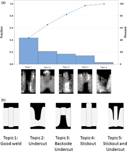
The resulting Pareto chart with the images which define the LDA-derived clusters or topics is given in Figure 1a. In the chart, the clusters or topics are themselves represented as images. Each topic is defined by the posterior means for the pixel or “word” probabilities. The charted quantities are the estimated posterior cluster proportions based on formulas in Appendix A.3 and Allen, Xiong, and Tseng (2020).

The inquirer sought to prioritize welding conformance issues and trace their sources. The Pareto chart provides a graphical overview of the LDA-derived clusters or topics in a ranked descending order from left to right. By linking these topics to known conformance issues from ANSI/AWS, the chart helps to highlight the most prevalent quality issues and prioritize each issue that needs to be addressed. Through visual comparison of the five topics illustrated in Figure 1a with ideal standards in Figure 1b, we can infer that the conformance issues in the Pareto chart, from topic 1 to topic 5, are “undercut,” “stickout,” “good weld,” “backside undercut,” and “stickout and undercut,” respectively.

The cluster with the largest proportion, topic 1 “undercut,” is associated with burn-through welds, suggesting that the power level of laser welding is an important cause (represented by the X-variable, which is defined in the following section) and that a reduction at this level is worthy of investigation. The analysis via image clustering and the Pareto chart underscores the necessity to prioritize the issue of laser welding power levels. This analysis sheds light on the problem and its context and facilitates the formulation of hypotheses for further research. Addressing this power level issue could potentially lead to a substantial decrease in nonconformity by more than 43 percent, thereby significantly mitigating a primary quality challenge in welding operations.

The principles and framework of EIDA

This section reviews the purposes of both EDA from De Mast and Trip (2007) and ETDA from Allen, Sui, and Akbari (2018), and then extends to the special context of image analysis, that is, EIDA. Also, we clarify our extension of their framework. As noted by those authors, the main purposes of EDA are “to generate hypotheses,” “to generate clues,” “to discover influence factors,” and “to build understanding of the nature of the problem.” Like the EDA and ETDA framework, the aim of the EIDA framework is to identify the potential relationships between key process output variables in six sigma terminology or Ys and the associated key process input variables or Xs with image data. To formalize this purpose, the following principle is proposed:

A. The purpose of EIDA is to leverage images for the identification of dependent variables, Ys, and independent variables, Xs, that may prove to be of interest for understanding or solving the problem under study.

De Mast and Trip classified the situations where the EDA is employed into two cases. In the first case, it is easy to identify the key output variables (Ys) and usually there is no straightforward way to parameterize the problem under study. In this case, the total negative instances, for example, defects, incidents, or other quality measures, can be decomposed as a sum of available categories of instances: (1) $$Y=Y_1+Y_2+Y_3+\dots$$(1)

In these situations, EDA (and EIDA) should be able to identify the dominating Y-variables and associate hypotheses for clear subsequent activities. The first example in Figure 1 shows how EIDA identifies dependent variables (Ys), representing welding conformance issues, for further study using image processing and a popular generative clustering method called LDA. The total number of welding with conformance issues (Y) can be decomposed as a sum of four types of conformance issues ($Y_1,Y_2,Y_3,Y_4$), namely “undercut,” “stickout,” “backside undercut,” and “stickout and undercut.” Image processing and LDA are described in more detail in Appendix A.

In the second situation classified by De Mast and Trip (2007), the total negative instances are seen as the aggregate of a large number of causal effects, where a lower level of attribution and analysis is needed. Then, the total negative events are written: (2) $$Y=E_1+E_2+E_3+\cdots \mathrm{ }$$(2) where $E_i=f(X_{j1},X_{j2}, X_{j3},\dots )$ denotes the effect of possible causes. The inquirer could acquire clues about $E_i$ by analyzing the images with respect to independent variables (Xs). Both Example 1 and Example 2 exemplify the application of EIDA in identifying clues for further investigation of independent variables (Xs). In Example 1, EIDA helps discern that the probable cause of the “undercut” issue in welding might be the power level of laser welding, which acts as an X-variable. On the other hand, Example 2 uses EIDA to unravel problems related to vision measurement and fixture distortions in robotic cells, again represented as X-variables.

Building upon the three-step process for quality improvement-related EDA framework proposed by De Mast and Trip (2007), one additional (initial) step of image processing to handle the complexities of image data and derive the quantitative data (denoted as Zs) for subsequent analysis. The process of EIDA can also be divided into four steps:

1. Image processing.

2. Image-derived quantitative data analysis and display.

3. Salient feature (pattern) identification.

4. Salient feature (pattern) interpretation.

The following sections provide additional principles, B–E, that build upon those discussed in De Mast and Trip (2007) and explain how the principles apply to these steps. These principles are systematically arranged in Table 1 for easy reference.

Table 1. Overview of the EIDA principles.

A. The purpose of EIDA is to leverage images for the identification of dependent variables, Ys, and independent variables, Xs, that may prove to be of interest for understanding or solving the problem.

B. EIDA is about extracting comprehendible and reproducible information from images, an inherently complex data source. Therefore, each step of the EIDA process should be simple, transparent (i.e., easy to understand and communicate), and robust to the peculiarities of variation in images such as the need for spatial invariance and correcting for the various types of distortion. B1. Image preprocessing methods for EIDA should be simple using standard methods for denoising, contrast enhancement, and segmentation including edge detection. B2. Features extracted from images for EIDA should be as repeatable as possible, which means not only representative but also invariant to variations such as scale, translation, rotation, angle, and illumination level. B3. Apply methods to tag images with numbers such as membership. These are useful for plotting and hypothesis generation. B4. Apply a simple and relatively transparent image spatial calibration to transform the image units or values to real-world measures for further analysis.

C. Process and display the image-derived quantitative data to reveal distributions and potential hypotheses paving the way for system quality improvement. C1. (Stratified Data). Process and display the image-derived quantitative data to reveal distribution across and within strata. C2. (Data plus time order). Process and display the image-derived quantitative data such that they will reveal distribution throughout the whole-time duration. C3. (Data plus spatial information). Process and display the image-derived quantitative data such that they will reveal distribution over spatial space. C4. (Multivariate data). Process and display the image-derived quantitative data in a low-dimensional subspace.

D. Search for deviations or variations from reference standards. D1. (Stratified data). Look for deviations or variations from other groups. D2. (Data plus time order). Look for deviations or variations from previous time intervals. D3. (Data plus spatial information). Look for correlation over space or look for deviations or variations from nearby locations. D4. (Multivariate Data). Look for correlation among variables. D5. Look for deviations or variations from prior perception, rules, or knowledge.

E. The identified salient features (patterns) should be interpreted using context knowledge. This knowledge can help in understanding the causes resulting from the vision system and the production process.

Image processing

Images and videos are frequently generated in a variety of applications and contain a vast amount of information. Image processing techniques, which have been developed in disciplines such as computer science, statistics, and applied mathematics (Qiu 2018), can be used to improve image quality and extract useful information from these data. These techniques, including denoising, enhancement, edge detection, and clustering, are commonly used in industry for various purposes and can be valuable for quality assurance. The primary goal of image processing is to derive quantitative data (Zs) to facilitate further data analysis, visualization, and hypothesis generation.

The procedure to conduct image processing used in our examples can be generalized into the following three steps:

• Step 1. Image preprocessing. After images are captured by sensors, image preprocessing converts them into a form that is more suitable for subsequent analysis through various operations such as restoration, denoising, contrast enhancement, sharpening, and region-of-interest detection and processing. Image segmentation is then used to isolate the desired object from the image for further analysis, leading to more precise analysis and reduced complexity. Edge detection is one example of segmentation.

• Step 2. Image feature extraction (Data reduction). After preprocessing and desired segmentation have been performed, image feature extraction techniques are applied to extract relevant features from the images for further analysis. Image feature extraction aims to transform high-dimensional images into lower-dimensional feature vectors, which can be considered a special case of data reduction. Typically, key geometric properties of the region, including shape, boundary, compactness, as well as texture, are crucial features to be extracted.

• Step 3. Additional processing with clustering or image spatial calibration to convert extracted image features into interpretable quantitative values (if appropriate). The image features extracted in step 2 may not be interpretable or meaningful to human perception. Clustering or image calibration are the primary techniques for additional processing to address this issue. Clustering methods typically generate visual words or “tags” for document clusters, while calibration converts the image units into meaningful physical measurements.

For more detailed information about the techniques of each step, please refer to Appendix A. One key aspect of images is the unique ability to provide direct visual causal insights in a way that other types of data, such as numerical or text data, cannot. Although the field of image processing contains many complexities, the general focus of EDA, as emphasized by both Tukey (1977) and Good (1983), is on simplicity and transparency. As a result, the second (new) principle of EIDA is as follows:

B. EIDA is about extracting comprehendible and reproducible information from images, an inherently complex data source. Therefore, each step of the EIDA process should be simple, transparent (i.e., easy to understand and communicate), and robust to the peculiarities of variation in images such as the need for spatial invariance and correcting for the various types of distortion.

The above principle can be decomposed into the following four sub-principles, B1–B4.

B1. Image preprocessing methods for EIDA should be simple using standard methods for denoising, contrast enhancement, and segmentation including edge detection.

In Example 2, we follow this principle, applying a simple image preprocessing step following this principle, we use to enhance the quality of the images. First, we use a Gaussian filter to denoise the images, followed by applying the linear contrast stretching to enhance the contrast. Subsequently, we segment the desired region (such as edges) for further image feature extraction.

B2. Features extracted from images for EIDA should be as repeatable as possible, which means not only representative but also invariant to variations such as scale, translation, rotation, angle, and illumination level.

The feature extracted from images should be representative, reflecting the intrinsic structure of the target region, including boundary, shape, and texture. Moreover, these image-derived features should be either robust to the above variations, or the variations can be compensated for with preprocessing techniques, particularly when dealing with raw images acquired in challenging conditions, such as dynamic environments and varied locations. For instance, similitude moments, one type of spatial moment that is often used to reflect the region shape, are invariant to translation and scale change.

In Example 2, edge detection highlighting the important structures of abrupt intensity changes indicates the boundary of the target area in the image. Although variations in illumination can bring challenges to edge detection, preprocessing techniques such as smoothing, and contrast enhancement can be used to normalize the image and compensate for these variations. In Example 3, the Frobenius norm (i.e., the sum-squared values) of horizontal, vertical, and diagonal detail coefficients based on Haar Wavelet Transform, serves as powerful low-dimensional descriptors to represent the image’s texture of energy in that direction. While the features based on Haar Wavelet Transform exhibit only translation invariance, we possess prior knowledge that the pipeline camera remains steady, and that there is minimal variance in the environment. Therefore, most of the captured images are expected to remain relatively consistent. These features remain favorable for the specific case of our pipeline inspection study.

Image-derived features are not aligned with how humans perceive images. Once robust and representative image-derived features are generated, additional processing of image tagging, and spatial calibration are preformed to produce quantitative data and facilitate hypothesis generation. This leads us to principle B3 and B4:

B3. Apply methods to tag images with numbers such as membership. These are useful for plotting and hypothesis generation.

Image clustering methods generally create visual words or “tags” for document clusters and numerical values to facilitate further data exploration steps. LDA, a method for unsupervised text and image clustering and automatic tag generation, is widely used and well-known (Blei, Ng, and Jordan 2003). LDA involves fitting a distribution to the words with probabilities often through Bayesian estimation of the chances that a randomly selected word is in a cluster (or “topic”) and that a randomly selected word in a specific document is assigned to that topic.

LDA uniquely differs from conventional statistical clustering techniques in that LDA decomposes each unit into several contributing topics, rather than assigning each observational unit (be it text or image) to a single discrete cluster (as in a multinomial mixture-based latent class analysis). This unique characteristic allows for a more nuanced understanding of the data. As it considers the potential multiple topics that might contribute to each observation, LDA provides a more refined and detailed analysis, beneficial in identifying quality issues at a higher resolution than traditional clustering analysis. In Example 1, we apply LDA to derive five topics and tag each image with a topic distribution thereby breaking down the overarching quality issue into five subtopics for further investigation. For those interested in the mathematical and computational details of LDA, please refer to Appendix A.3.

B4. Apply a simple and relatively transparent image spatial calibration to transform the image units or values to real-world measures for further analysis.

Quality control projects often involve inspecting the size, shape, location, or defective level of objects. The measurements we extracted from images are based on image units (pixels). Calibration converts the image units to physical measurements and offsets the variation on the scale. Many calibration methods have been proposed to transform 2-D images into 3-D real-world coordinates. (Tsai 1987; Zhang 2000). Intensity or color values calibration is also of interest when these values correspond to some property of the studied object (Nederbragt et al. 2005, 39–43). In Example 2, a second-order regression model is built to model the relationship between measurement in pixel units and real-world gap and flush values. This model allows us to convert measurements to their corresponding real-world measures.

In general, our objectives for image tagging and spatial calibration are to produce quantitative data (Zs) that facilitates hypothesis generation. The next sections illustrate how the derived outputs can be visualized to aid in quality improvements.

Image-derived data analysis and display

After preparing image-derived features or image-creating numbers relating to cluster identities, one can follow steps 2–4 which derive from the methods of De Mast and Trip (2007). Then, graphical presentation in EIDA offers an effective tool to emphasize and present findings to analysts (Good 1983; Hoaglin, Mosteller, and Tukey 1983; Bisgaard 1996). Therefore, after image processing, the next step is to display image-derived quantitative data (Zs) in a straightforward way that exploits the human visual capability of pattern recognition.

C. Process and display the image-derived quantitative data to reveal distributions and potential hypotheses paving the way for system quality improvement.

Graphical presentations, as noted by Bisgaard (1996), can reveal patterns in the data that may not have been anticipated before analysis. For EIDA, revealing patterns can pertain to the distribution of the resulting quantitative data from image processing or the distribution of the visual words (visual words can be pixels or image feature descriptors) across specific topics (clusters). At this phase, the primary visualization tools such as Pareto charts or sorted bar graphs, running charts, histograms, and others can be used to display image-derived quantitative data, different topics, and topic proportions. Note that in Figure 1a, the topic proportions are captured and represented in descending order through Pareto charts. The inquirer could examine the topics from the largest probability to the least and, therefore, elucidate the priority of each specific issue.

C1 (Stratified Data). Process and display the image-derived quantitative data to reveal distribution across and within strata.

As noted by De Mast and Trip (2007), stratification plays an important role in data visualization to identify and control confounding factors. After stratification, the confounder does not vary within each stratum. Through this principle, EIDA can help the inquirer narrow down the search range for the quality issue by focusing on a certain stratum. Thus, practitioners can use visualization tools such as box plots for each stratum to generate hypotheses for further investigation, as illustrated in Example 2.

A special type of confounder explored by De Mast and Trip (2007) is the temporal confounder, which might lead to bias in further hypothesis generation. The following principle is derived to overcome temporal confounders:

C2 (Data plus time order). Process and display the image-derived quantitative data such that they will reveal distribution throughout the whole-time duration.

Plotting data against time facilitates the search for important X-variables (Allen, Sui, and Akbari 2018). This principle is illustrated in the following Example 2, which also illustrates roles for trend plotting or control charts.

C3 (Data plus spatial information). Process and display the image-derived quantitative data such that they will reveal distribution over spatial space.

Plotting data against spatial space can direct the identification of causes (De Mast and Trip 2007). If spatial information is available, displaying the spatial distribution can assist in identifying atypical locations or uncovering interesting patterns of spatial associations. The following Example 2 illustrates this principle.

C4 (Multivariate data). Process and display the image-derived quantitative data in a low-dimensional subspace.

In the image processing section, we demonstrate that principal component analysis (PCA) can be used to project raw image data from high-dimensional arrays into low-dimensional feature space (also regarded as image compression). Similarly, if the initial feature vectors (image attributes) generated from image processing are still high-dimensional and far beyond human perceptive capability, one more step of dimensionality reduction can be implemented into these image attributes with projection methods like PCA or feature selection. The resulting low-dimensional data can be visualized by scatter plots, parallel coordinates plots, or contour plots of the empirical density. Example 3 serves as an illustration of this principle.

Salient feature identification

Once the distribution of image-derived quantitative data (Zs) is visualized, the next step in EIDA is the identification of the salient features (patterns), following the same process as EDA in De Mast and Trip (2007) and ETDA in Allen, Sui, and Akbari (2018). According to those authors, salient features in the data are the “fingerprints” of the possible effects of causes, which clarify the key X-variables. The idea of identifying salient features is defined by Shewhart (1931, 1939) as uncovering “the clues to the existence of assignable causes” for non-randomness. The causes being sought, therefore, often relate to deviations of system outputs from expected outputs or standards, which leads to the following principle:

D. Search for deviations or variations from reference standards.

In general, the resulting image-derived quantitative data is like normal numerical data in that deviation from the normality or a reference distribution can indicate the presence of salient features. Certain dominant causes of variation can also leave distinctive traces that can be used to identify salient features. In Example 2, Figure 2a illustrates a deviation (extreme value) from normality, indicating a salient feature. Another example of this principle is elaborated in Figure 8 of Example 3. The deviation from the reference distribution indicates the defects and other non-acceptable areas. Furthermore, the texture measure of energy in the image shows the discriminative power for effectively distinguishing the defect and other structural areas from the normal area.

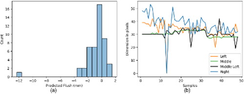
Figure 2. Investigation of quality issues on body-in-white door flush values: (a) distribution of predicted flushes on lower measurement points (positive and negative indicate the direction of flushes) and (b) the dimension in pixels computed from each camera to predicted flushes.

The strata (groups or locations) act as a “container factor” confounding the effect of many variables (De Mast and Trip 2007). The next principle is derived from the type of variation between groups.

D1 (Stratified data). Look for deviations or variations from other groups.

Boxplots can be used to examine variations among different strata. As shown in Figure 5 of Example 2, the distribution of gaps at the top of the door (labeled with “A”) is significantly different from other locations. This suggests more attention needs to be given to this location to find the source causing dimensional deviation.

The following principle is derived from another type of deviation that relates to periods.

D2 (Data plus time order). Look for deviations or variations from previous time intervals.

Deviations from previous time intervals can be in the form of a trend, cyclical patterns, or shifts in the mean. Time series plots of image-derived quantitative data, such as cluster posterior probabilities (proportions) or dimensions, can facilitate the search for these deviations and potentially identify important X-variables. These could include a partial autocorrelation function, decomposition plots of trend, seasonality, and noise components, or a run chart.

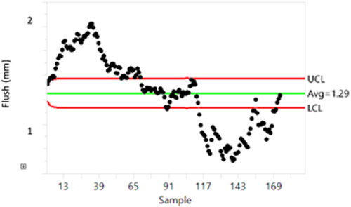
Example 2 illustrates the use of an EWMA (exponentially weighted moving average) control chart in flush measurements revealing a salient feature. EWMA control charts are described in detail in Appendix C. In this case, the salient feature (pattern) relates to the distortion of the fixtures used in robotic cells. In the case of multiple time series that need to be studied simultaneously, plotting them on the same chart and comparing them helps to discover the correlations between multiple time series.

D3 (Data plus spatial information). Look for correlation over space or look for deviations or variations from nearby locations.

Example 2 illustrates this principle. The spatial distribution of dimension measurements is presented in the image of the BIW car body. The deviations of atypical locations from nearby locations narrow down the research range and indicate that more attention should be focused on investigating the source of variation at these locations.

D4 (Multivariate Data). Look for correlation among variables.

As stated in principle D2 for multiple time series, plotting multiple time series at the same time to look for correlations is suggested. The same idea applies to multivariate data. Examining the correlations among variables facilitates inquirers to discover the important dependent variables (Xs) and the relationship between Xs and Ys.

D5. Look for deviations or variations from prior perception, rules, or knowledge.

Prior knowledge of practitioners or inquirers can assist in identifying the salient features (patterns). This principle is illustrated in the later Example 2 to analyze the flush distribution. The presence of an extreme flush value suggests that more investigation should be conducted on the vision system rather than the production process with the prior knowledge of the practitioner.

As described in De Mast and Trip (2007), the final principle related to the interpretation of salient features:

E. The identified salient features (patterns) should be interpreted using context knowledge. This knowledge can help in understanding the causes resulting from the vision system and the production process.

In this step, context knowledge is used to develop hypotheses from salient patterns. The concept of abduction was originally introduced by Charles Peirce (Niiniluoto 1999; De Mast and Bergman 2006), in which “the inquirers compare conceptual combinations to observations until all the pieces seem to fit together and a possible explanation pops up.”

Example 2 also illustrates this principle in that the context knowledge of partitioners helps eliminate the assembly process as a potential cause of extremely abnormal measurements in flush levels. This ultimately led to the realization that the issue was likely related to a problem with the camera.

Illustrative examples

In this section, the application of EIDA principles and methods is illustrated with three additional examples. These examples demonstrate the process of generating hypotheses about key input or output variables and identifying the potential causes of quality issues. These generated hypotheses direct practical decision-making and problem-solving.

Example 2: Body-in-white dimensional study

This case concerns the BIW vision measuring project for measuring the gaps, flushes, and door alignment on the car body with computer vision to support assembly inspections and improve the quality of measurements. The gap refers to the horizontal distance or separation between two surfaces on a car body, while the flush represents the vertical displacement or offset between the two surfaces in the perpendicular direction. Door alignment involves measuring the vertical misalignment between the beltline heights of the front and rear doors when they are closed. This measurement is typically accomplished by assessing the vertical misalignment of specific corner points, such as the B location illustrated in Figure 3.

Figure 3. Estimation process for upper car door gap (A) and misalignment (B): (a) edge detection, (b) region identification and the dimension in pixels, and (c) raw image with predicted gap and misalignment.

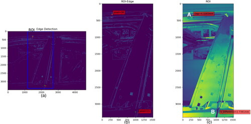
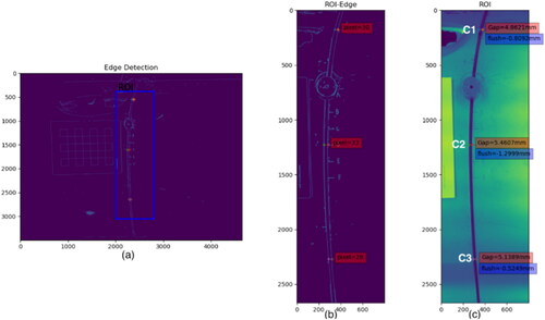
Two groups of cameras (totaling of 8 cameras) are set to capture the images for 5 measurement locations from different angles (left, middle left, middle, and right). One group is to capture images of the upper door gap and door misalignment as presented in Figure 3. The other group is to capture three lower gaps and flushes as presented in Figure 4. Image processing is applied to each image to obtain the dimensions of gaps, flushes, and misalignment.

Figure 4. Estimation process for lower car door gaps and flushes of locations (C1–C3): (a) edge detection, (b) region identification and the dimension in pixels, and (c) raw image with predicted gap and flush.

We followed the standard image preprocessing procedure to remove noise, locate the regions of interest (ROIs) area, detect the edge structure of BIW, and finally output the dimension in pixel units, for each measurement location. The Canny method is used for edge detection and is described in detail in Appendix B. For each measurement, a second-order regression model with interaction term is used for spatial calibration to convert the dimension in pixels into physical units. This model is formulated to represent the relationship between the dimension in pixels from different angle images $C_i$ ($C_1,$ $C_2$ and $C_3$ denote the dimension in pixels derived from left, middle, and right cameras) and known real-word dimensions $S$ according to Eq. (3)(3) $$S={\beta }_0+{\beta }_1{C}_1+{\beta }_2{C}_2+{\beta }_3{C}_3+{\beta }_4{C}_1{C}_3+\epsilon$$(3) : (3) $$S={\beta }_0+{\beta }_1{C}_1+{\beta }_2{C}_2+{\beta }_3{C}_3+{\beta }_4{C}_1{C}_3+\epsilon$$(3) where ${\beta }_j \left(j=0,1,2,3,4\right)$ describes the regression coefficient, ${\beta }_0$ is a constant term describing intercept, and $\epsilon$a disturbance term describing the residual error.

The method of ordinary least squares provides the estimate of coefficients. Then, we use the fitted model to predict the physical dimensions for new runs. Aligning with principle B4, the predicted dimensions in real-world units in millimeters are easier for human perceptions than raw image pixels.

The histogram of Figure 2 shows the distribution of 48 predicted flush measurements. Upon inspecting the distribution, an abnormal measurement of −12 mm is observed, which deviates greatly from the general expected distribution. This deviation suggests a salient feature (pattern) relating to the measurement system. This measurement is also at odds with what the inquirer expected. According to the knowledge of car assembly workers, such an extremely large amount of flush cannot occur during production, indicating that the abnormality might be a result of a vision system issue. By plotting the dimension in pixels of each camera (the input features of the regression model) in Figure 2b, the failure of the left and right cameras emerges, as indicated by zero values around index 13. This reasoning illustrates how to use the principle of D5 and E to search for salient features and interpret them using prior context knowledge.

The resulting images, labeled with the dimension in pixels and predicted physical dimensions, are given in Figures 3 and 4. The spatial distribution of gaps, differing by over 1 mm, suggests that the location at the top of the door (location A in Figure 3c) likely needs more attention than locations at the bottom of the door (Figure 4c). This suggests that the relatively small gap is the key Y-variable for improvement activities. By inspecting Figure 4c, clearly, both the gap and flush of the middle location (C2) are larger than the two neighboring locations (C1 and C3), implying a dimensional deviation in spatial space. A hypothesis can be formed that investigating the source of this deviation may lead to an improvement in gap quality and the overall assembly process. This is the case in which image resulting data are used to help uncover the causes (key X-variables) by visualizing and comparing dimensions over space.

Boxplots of gap dimensions for each location in Figure 5 show the distribution within and across strata. The differences in distribution among the four locations are salient and the large variance observed within the location at the top of the door provides a clue for identifying potential quality issues with the gap. Looking over the time of many months in Figure 6, we see a clear evolution of the smoothed flush value from an EWMA control chart. More details about the EWMA control chart are described in Appendix C. This chart suggests that deviations from nominal values are accruing and not being effectively counteracted at the time scale of many months. This potentially rules out many possible sources of deviation and focuses attention on accumulating deviations likely related to the distortions of the fixtures used in the robotic cells.

Figure 5. Gap dimension distributions for body-in-white by measurement location.

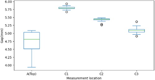
Figure 6. EWMA control chart of predicted flush values (some data are changed to protect the source but show trends in flush over time from drifting robotic fixtures).

Example 3: Pipeline defect study

In this study, we analyze approximately 2,500 sections of oil and gas pipelines, each of which potentially represents a “defect” or amount of corrosion requiring immediate repair. The leftmost image of Figure 7 shows a sample magnetic flux leakage image of a defective section in the pipeline.

Figure 7. Wavelet transformation and Frobenius norms computed for a pipeline wall image.

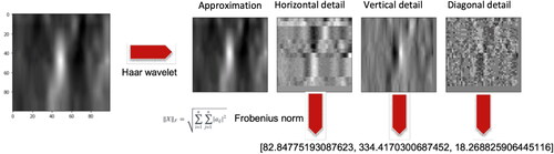
To understand the distributions of defects in pipelines, the Haar wavelet transform is used to extract image features, as it provides powerful insight into the spatial-frequency characteristics in the horizontal, vertical, and diagonal directions (Ghorai et al. 2013). Figure 7 illustrates the approximation coefficients and detail coefficients of three directions at level 1. The Frobenius norm, or the sum-squared values, of each detail coefficient (represented as pixel darkness values in the image of Figure 7) serves as low-dimensional descriptors to represent the image’s texture of energy in that direction. These texture descriptors can aid in understanding the distribution of images.

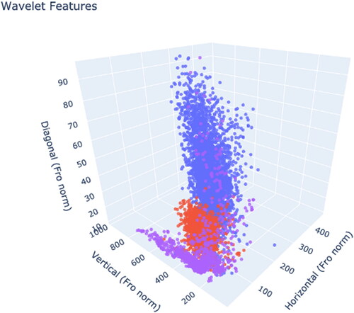
Figure 8 shows how the Frobenius norm values of the candidate defective area images can aid in understanding the distributions of defects, normal sections, and other structural sections (weld or installation patches) in the data. We omit the labels to protect the confidentiality of the sponsor’s data. Yet, if we take one group as the reference distribution, the deviation of the other two groups from the reference can be visualized. This also implies that the Frobenius norm of three directions of detail coefficients, especially horizontal direction, based on the Haar Wavelet transform, is powerful in discriminating the defects or non-normal sections from normal sections. This case suggests that the deviation in horizontal texture from normal sections reveals clues of salient patterns regarding pipeline quality, that is, the causes of defects relate to diagonal feature creation presumably because vertical and horizontal features relate to purposeful structural features.

Figure 8. Classifying images using Frobenius norm values of wavelet coefficients for pipeline inspection. Data were generated from three groups: acceptable pipe sections (normal), defective sections, and other structural sections.

Final remarks

This article describes the application of the EDA framework of De Mast and Trip (2007) to image data. The resulting EIDA principles are developed through examples from real-world quality improvement studies. First, the purpose of the overall analysis is formalized. Then, EIDA involves an initial “image processing” step which could involve preprocessing (denoising, image enhancement, segmentation), image feature extraction, and an additional procedure of clustering or image calibration which transforms the image or non-informative feature into meaningful quantitative inputs for further analysis.

The sets of proposed principles and methods first relate to the identification of key input (Xs) and output (Ys) variables (A), then the second relates to using simple and transparent image processing procedures (B), third relates to studying the nature of the variation with graphical presentations (C). Then, methods for investigating deviations from a reference standard are studied (D) and finally, methods for exploring and interpreting the salient features (patterns) are presented (E).

We developed EIDA with various projected tasks: welding inspection with low-resolution but portable weld images, dimensional measurement with multiple angles of BIW images, and pipeline defect detection with magnetic flux leakage images. We hope that the principles, methods, and diagrams presented here may serve as a standard part of the analysis process for these types of tasks and various input images. Then, more promising hypotheses about the causes of quality problems and avenues for improvements may be generated, in part because the framework allows the use of an analytical mindset that is commonly used with other types of data to be applied to image data.

Many topics are available for future research. This EIDA focuses on the collected discrete image data. EIDA on videos, considered as a composition of images, follows the same general process and principles, but its temporal nature can be exploited with additional motion analysis or frame-by-frame analysis. Future work can extend EIDA to video data. Further investigation can reveal useful routines in software commonly used by quality professionals, such as R, Python, SAS, JMP, and SPSS Modeler.

Acknowledgments

We are grateful to Shubho Bhattacharya, Ravish Eshwarappa, John Jaminet, and Jeremy Galante for their insights and support relating to BIW quality. We also express our gratitude to Dirk Maiwald, Christoph Hermes, and Jonas Meyer for their insights and support relating to pipeline monitoring. Special appreciation goes to Zhenhuan Sui for his critical support.

Disclosure statement

No potential conflict of interest was reported by the author(s).

Additional information

Funding

This work was supported by the Honda of America Manufacturing [Award No. 114252] and ROSEN Group [Award No. 112489].

Notes on contributors

Yifei Zhang

Yifei Zhang is a Ph.D. student in Integrated Systems Engineering at The Ohio State University. She is the author of four Chinese patents relating to fault diagnosis systems. Her research interests include quality engineering, nonlinear programming, sensor analytics, vision AI, and image analysis.

Theodore T. Allen

Theodore T. Allen is an professor of Integrate Systems Engineering at The Ohio State University. He received his Ph.D. in Industrial Operations Engineering from the University of Michigan. He is the author of over 70 peer-reviewed publications including two textbooks. He is the vice president of Communications for the INFORMS PSOR section and a simulation area editor for Computers & Industrial Engineering. He was a 2023 finalist in the INFORMS Edelman Award Competition for his work with the DHL Supply Chain company.

Ramiro Rodriguez Buno

Ramiro Rodriguez Buno is a Ph.D. student in Integrated Systems Engineering at The Ohio State University. His research interests include quality engineering, operations research, AI, and digital manufacturing.

Appendix A:

Image processing

A.1 Image preprocessing

Once the images or videos have been acquired with sensors or cameras, the first step is image preprocessing. Image preprocessing methods may be grouped into four classes of operations: image correction or restoration (to compensate the data error, image noise, and geometric distortion and improve the appearance of an image), image enhancement (to emphasize certain desired image features for specific application), morphological processing (to extract image components that are useful in the representation and description of region shape [Gonzalez and Woods 2018, 42]) and image segmentation (to partition an image into regions or segments).

a. Image correction or restoration

Image correction or restoration is the process that attempts to recover a degraded image by modeling the degradation with prior knowledge (Gonzalez and Woods 2018, 317). The known degradation comes in many forms such as noise, blur, and distortion.

Noise could be introduced into an image during acquisition or transmission, due to the uncertainty of environmental factors, such as light level, sensor temperature, or due to channel interference of transmission. Spatial filters such as mean filter, geometric mean filter, median filter, Gaussian filter, and frequency domain filter such as notch filter could be used to remove specific types of noise. The period noise, typically generated from electrical interference during acquisition, can be modeled with the Fourier spectrum.

In the case of blurring, it is possible to estimate the actual blurring and take the inverse transform to deblur the image. Geometrical distortions, such as skew, radial distortion, and tangential distortion, are also common issues that image systems undergo. These distortions originate from two distinct sources: internal distortion (resulting from the geometry of the sensor) and external distortion (resulting from the perspective of the sensor or the non-flat shape of the object). Geometric correction is required to correct the distortion before future analysis.

b. Image enhancement

Image enhancement aims to highlight certain image features and weaken or remove trivial information or noise for later analysis. Image restoration and enhancement both aim to improve the appearance of an image, but while the restoration is based on mathematical or statistical modeling with prior knowledge, enhancement is more subjective and based on human preference. Common techniques used in image enhancement include image smoothing, sharpening, contrast enhancement, and processing specific regions of interest (ROIs).

Image smoothing aims to attenuate the sharp transition in intensity while image sharpening aims to highlight intensity changes and emphasize fine details in images. Both image smoothing and sharpening can be achieved using either spatial domain or frequency domain filters. Spatial filters used for image restoration, such as the Gaussian filter, can also be used for image enhancement to smooth images and reduce noise. The usage of image sharpening is widespread in industrial inspection, including in detecting surface defects on products. This technique enhances the visibility of edges and subtle irregularities, thereby bolstering defect detection efficiency. Image sharpening techniques include first-order derivative operators (e.g., Sobel, Prewitt) and second-order derivative operators (e.g., Laplacian filter) in the spatial domain. First-order derivative operators are less sensitive to noise and typically yield thick edges corresponding to slow variations in intensity. This characteristic can be advantageous in certain applications, such as when the quality of the original image is poor. Conversely, second-order derivative operators generate double edges, each of them one-pixel thick and separated by zeros, yielding sharper contrasts. This feature makes them particularly useful in applications requiring high precision. In the frequency domain, low-pass filters can be used to smooth images by attenuating high frequencies and preserving low frequencies, while high-pass filters can be used to sharpen images by suppressing low frequencies and passing high frequencies.

Contrast enhancement is a technique used to improve the interpretability of images by redistributing their intensity values. Low-contrast images may be caused by poor illumination and have intensity values limited to a narrow range. Contrast enhancement expands this range to the entire intensity range of [0, 255]. There are two main types of contrast enhancement: linear contrast stretch and nonlinear stretch. Minimum–maximum stretch is a linear method that maps the maximum brightness value to 255, and the minimum value to 0, and scales all intermediate values proportionally between 0 and 255. Histogram equalization is a nonlinear method that redistributes intensity values to follow a uniform distribution. This method is often effective in producing images with the most contrast of any enhancement technique (Reddy 2018, 110).

Sometimes, instead of working on a whole image, a specific subregion of an image is more of interest, typically referred to as the region-of-interest (ROI) processing. Template matching is one of the techniques used for ROI detection using similarity scores such as normalized cross-correlation (NCC). After filtering out the ROI area from the original image, various image processing techniques such as noise reduction, smoothing, and sharpening can be applied to this ROI area.

In Example 2, the images of the BIW are first smoothed using a 5 × 5 Gaussian kernel to remove noise. Then, the template matching method with the NCC score is used to identify the ROI area for the target measurement location. Finally, linear contrast stretching is applied to the ROI to enhance the brightness contrast and make the edges of the BIW more visible.

c. Morphological processing

Morphological processing describes a set of operations that process images based on the shape (or morphological features) of an image, typically for binary images. The two fundamental operations are dilation, which enlarges the binary region by filling the small holes or cracks, and erosion, which shrinks the binary region by removing small objects.

Composite operators, such as closing and opening, can be created using these two fundamental operations to avoid the general shrinking or enlarging of the object size. Closing is achieved by performing dilation followed by erosion, while the opening is achieved by performing erosion followed by dilation. These two operations tend to remove the small objects or fill the holes with smooth boundaries. Example 2 uses an opening operation to enhance the shape of binary edges by removing the small, disconnected edge points.

d. Image segmentation

Image segmentation is the process that partitions an image into distinct regions, called segments, concerning certain criteria. There are two main approaches to partitioning images into segments: one based on sharp intensity discontinuities (typically indicating edges), and another based on the similarity of pixel attributes, such as intensity or color values.

Edge detection is a method used to detect abrupt discontinuities in intensity in an image and identify edges. After edge detection, a linking algorithm is applied to assemble detected edge pixels into more meaningful edges, which typically indicate the boundaries of regions or objects. Common techniques for edge detection include Prewitt, Sobel, Canny, Roberts, and Laplacian operators. These techniques can also be used for image sharpening. The Canny method, which could produce thin, clean, and precise edges, is used in Example 2 to extract two edges of gaps and flushes in BIW images. More details regarding the Canny edge detector are described in Appendix B. Thresholding, region-based segmentation including region growth, clustering, and “superpixels” are the examples that fall into the second type of segmentation.

A.2 Image feature extraction (data reduction)

The main objective of image feature extraction is to obtain significant information from the original image and represent that information in a lower-dimensional feature space. Image feature extraction consists of two aspects: feature detection and feature description. Feature detection refers to finding features in an image, region, or boundary, while feature description refers to describing the detected features with quantitative values. For example, a corner in an image could be detected as an interesting point and described with its location and gradient.

The image feature extraction methods can be broadly divided into two categories: region (Local), and whole images (Global). Some features can be applied to both categories. After the region is identified from the image segmentation step, feature extraction is applied to the region. The geometric properties of the region to describe shape can be represented by its boundary, bounding box, skeleton, area, compactness, moment invariants, etc.

The texture is an important aspect of image analysis that can provide valuable information about the properties of a region. Statistical moments of the intensity histogram of an image or region can describe the texture of smoothness, coarseness, etc. (Gonzalez and Woods 2018, 846). For instance, the second-order moment (i.e., the variance of intensity) can be used to formulate the descriptor of the relative intensity smoothness. Yet, these descriptors computed on intensity or color (RGB) histogram alone miss the spatial relationships between pixels. To incorporate spatial information, descriptors, such as correlation, compactness, entropy, and so on, can be computed on a co-occurrence matrix of pixels instead of an intensity histogram. The Fourier spectrum is used primarily to describe the texture in the frequency domain. For instance, a periodic pattern of the images or region can be represented with a peak in the Fourier spectrum.

The wavelet transforms, the classical multiscale signal processing method, are also frequently used for texture feature extraction but in the spatial-frequency domain. Examples of wavelets include Haar, Daubechies, Mexican hat, etc. The wavelet coefficients of each level are used to build the image feature vectors. Chang and Ravathur (2005) used wavelet decomposition to obtain the signature of an anisotropic steel specimen surface and predict the surface roughness. In Example 3, the Haar wavelet transform is applied to extract texture information of pipeline images in horizontal, vertical, and diagonal direction. Then, the Frobenius norm of each direction coefficient, is computed and serves as powerful low-dimensional descriptors to represent the image’s texture of energy in that direction. The Haar wavelet is described in more detail in Appendix D.

The above texture features can also be used for whole images. Besides that, FAST (features from accelerated segment test), Harris detector, and SIFT (scale-invariant feature transform) are well-known image feature extraction methods that apply to the entire image to detect interest points and generate image features. FAST Developed by Rosten and Drummond (2006) and the Harris detector formulated by Harris and Stephens (1998) is a are two popular corner detection methods. SIFT transforms an image into n-dimensional feature vectors that are invariant to scale, transformation, and rotation, and robust to affine distortion and illumination. Other approaches introduced into image feature extraction include principal component analysis (PCA), manifold learning, bag-of-visual-words (also known as bag-of-features) model, etc. Example 1 uses bag-of-visual-words to represent a region or image as an unordered collection of pixel indices and feed to the clustering model.

A.3 Additional processing with clustering or image calibration

The raw image feature extraction may extract abstract and non-interpretable features which are not in line with human perception. For instance, the bag-of-words in Example 1 is defined with the histogram of pixel indices, and the extracted measurements (such as size, distance, etc.) from images in Example 2 using spatial units just in “pixels” instead of real-world spatial units (mm, cm, etc.). These types of image-derived features are not aligned with how humans perceive images. Additional processing of the clustering model or image calibration is needed to address this issue.

a. Latent Dirichlet allocation (LDA) topic clustering

The LDA model proposed by Blei, Ng, and Jordan (2003), is a generative probabilistic model of a corpus. This is the most cited method for clustering unsupervised images or text documents perhaps due to its relative simplicity and the interpretability of the resulting cluster or topic definitions (Rosen-Zvi et al. 2010). LDA is primarily concerned with the probabilities defining the clusters or topics (“topic probabilities”) and the probabilities relating to the association of words in specific documents with the topics (“document-topic” probabilities). The estimated posterior mean values of these defining probabilities can be used as inputs for further analysis. In image analysis, the term “documents” could be the images. The “words” could be the indices of the pixels in each image, the method that is used by Allen, Xiong, and Tseng (2020). The extracted image features such as vector quantized SIFT descriptors, local binary patterns, and Weber local descriptors could also play the role of “word” in LDA (Chen et al. 2009; Ahonen et al. 2006).

Assume that $w_{d,j}$ is the $j^{th}$ word in dth document with d = 1, …, D and j = 1, …, N_d, where D is the number of documents or images, and N_d is the number of words in the dth document. Therefore, $w_{d,j}\in \{1,\dots ,W\},$ where $W$ is the number of distinct words in all documents. The clusters or “topics” are defined by the estimated probabilities, ${\widehat{\varphi }}_{t,c},$ which signifies a randomly selected word in cluster t = 1, …, T (on that topic) achieving the specific value c = 1, …, W. Also, ${\widehat{\theta }}_{d,t}$ represents the estimated probability that a randomly selected word in document d is assigned to cluster or topic t. The model variables $z_{d,j}$ are the cluster assignments for each word in each document, d = 1, …, D and j = 1, …, N_d. Then, the joint probability of the word $w_{d,j}$ and the parameters to be estimated, ($z_{d,j}, {\theta }_{d,t},{\varphi }_{t,c}$), is: $$P(w_{d,j},z_{d,j},\mathrm{ }{\theta }_{d,t},{\varphi }_{t,c}{N}_d,\alpha ,\beta ,\mathrm{ }d=1,\dots ,D,\mathrm{ }t=1,\dots ,T,c=1,\dots ,W)=\left[\prod _{t=1}^T\frac{\Gamma \left({\sum }_{c=1}^W\beta \right)}{\prod _{c=1}^{WC}\Gamma \left(\beta \right)}\prod _{c=1}^W{\varphi }_{t,c}^{\beta -1}\right]\left[\prod _{d=1}^D\frac{\Gamma \left({\sum }_{c=1}^W\alpha \right)}{\prod _{c=1}^{WC}\Gamma \left(\alpha \right)}\prod _{t=1}^T{\theta }_{d,t}^{\alpha -1}\right]\times \left[\prod _{d=1}^D\prod _{t=1}^T{\theta }_{d,t}^{n_t^{\left(d\right)}}\right]\times \left[\prod _{t=1}^T\prod _{c=1}^W{\varphi }_{t,c}^{n_t^{\left(c\right)}}\right]$$ where $\Gamma \left(\dots \right)$ is the gamma function and: (4) $$\mathit{the }{n}_t^{(d)}={\sum }_{j=1}^{N_d}{\sum }_{c^{\prime }=1}^{W}I\left(z_{d,j}=t\mathrm{ }\&c=c^{\prime }\right)\text{ and }{n}_t^{(c)}={\sum }_{d=1}^D{\sum }_{j=1}^{N_d}I\left(z_{d,j}=t\mathrm{ }\&{\mathrm{ }w}_{d,j}=c\right)$$(4) and where $I(\dots )$ is an indicator function giving 1 if the equalities hold and zero otherwise.

Note Eq. [4] is a simple representation of human speech or images in which words, ${ w}_{d,j},$ and topic assignment, $z_{d,j},$ are both multinomial draws associated with the given topics. The probabilities ${\varphi }_{t,c}$ that define the topics are also random with a hierarchical distribution. The estimates that are often used for these probabilities are Monte Carlo estimates for the posterior means of the Dirichlet distributed probabilities ${\widehat{\theta }}_{d,t}$ and ${\widehat{\varphi }}_{t,c},$ produced by low values or diffuse prior parameters $\alpha$ and $\beta .$

To estimate the parameters in the LDA model in Eq. [4], “collapsed Gibbs” sampling (Griffiths and Steyvers 2004; Teh, Newman, and Welling 2007) is widely used. First the values of the topic assignments for each word $z_{d,j}$ are sampled uniformly. Then, iteratively, multinomial samples are drawn for each topic assignment $z_{d,j}$ iterating through each document d and word j using the last iterations of all other assignments $z_{-\left(d,j\right)}.$ The multinomial draw probabilities are (5) $$P\left(z_{d,j}=t{d,j,z}_{-\left(\mathit{d},\mathit{j}\right)},w_{d,j}\right)\propto \left(\frac{n_t^{\left(w_{d,\mathrm{j}}\right)}-I\left(z_{d,j}=t\right)+\beta }{n_t^{(·)}-I\left(z_{d,j}=t\right)+W\beta }\right)\left(\frac{n_t^{\left(d\right)}-I\left(z_{d,j}=t\right)+\alpha }{n_{·}^{\left(d\right)}-1+T\alpha }\right)$$(5) where $n_t^{(w_{d,j})}={\sum }_{d^{\prime }=1}^D{\sum }_{j^{\prime }=1}^{N_d}I\left(z_{d^{\prime },j^{\prime }}=t\mathrm{ }\&{\mathrm{ }w}_{d^{\prime },j^{\prime }}=w_{d,j}\right),$ $n_t^{\left(·\right)}={\sum }_{d^{\prime }=1}^D{\sum }_{j^{\prime }=1}^{N_d}I\left(z_{d,j^{\prime }}=t\right),$

$n_t^{(d)}={\sum }_{j=1}^{N_d}{\sum }_{c^{\prime }=1}^{W}I\left(z_{d,j}=t\mathrm{ }\&c=c^{\prime }\right),$ and $n_{·}^{(d)}={\sum }_{t^{\prime }=1}^T{\sum }_{j^{\prime }=1}^{N_d}I\left(z_{d,j^{\prime }}=t\right).$

In words, each word is randomly assigned to a cluster with probabilities proportional to the counts for that word being assigned multiplied by the counts for that document being assigned. After M iterations, the last set of topic assignments generates the estimated posterior means using: (6) $${\widehat{\varphi }}_{t,c}=\frac{n_t^{\left(c\right)}+\beta }{n_t^{(·)}+W\beta }$$(6) and the posterior mean topic definitions using (7) $${\widehat{\theta }}_{d,t}=\frac{n_t^{\left(d\right)}+\alpha }{n_{·}^{\left(d\right)}+T\alpha }$$(7)

Therefore, if words are assigned commonly to certain topics by the Gibbs sampling model, their frequency increases the posterior probability estimates both in the topic definitions ${\widehat{\varphi }}_{t,c}$ and the document probabilities ${\widehat{\theta }}_{d,t}.$

b. Spatial or density image calibration

Quality control projects often involve inspecting the size, shape, location, or defective level of objects. Once we extract dimensions from images, we can apply calibration to convert these dimensions into more meaningful units for real-world analysis. There are two types of calibration commonly used in these projects: spatial calibration and density calibration.

Spatial calibration seeks to convert the spatial units of pixels into real-world units such as millimeters or square millimeters. The classical calibration methods proposed by Tsai (1987) and Zhang (2000) are the most cited to estimate a camera’s intrinsic and extrinsic parameters by mapping the 3-D real-world coordinates and their projections in images with geometric transformation. Recently, more calibration methods based on statistical models or neural networks have been studied. In our example 2, a second-order regression model is built to model the relationship between measurement in pixel units and real-world gap and flush values.

The density calibration is also of high significance when the pixel values represent measurements such as the darkness of the ROI area, reflectance, or whatever the inspection task aims to measure. Density calibration converts the pixel values (density or color) to the above real-world measures. Before implementing further analysis, we need to build the mathematical relationship between pixel values and corresponding real-world measures with linear, polynomial, or more complex models if necessary.

In general, additional processing of clustering and spatial calibration aims to produce quantitative data to facilitate hypothesis generation.

Appendix B:

Canny edge detection

The canny edge detector proposed by Canny (1986) is a superior edge detection operator that uses multiple steps to achieve a better performance than most traditional edge detections, such as Prewitt operator, Sobel operator, etc. (Rong et al. 2014; Gonzalez and Woods 2018, 729). The canny method is derived based on three criteria of signal-to-noise ratio (SNR) maximization for good edge detection, good localization, and single-edge response. The general process of Canny edge detection consists of the following four steps:

Step 1: Smooth the image with the two-dimensional Gaussian functions. Let I(x,y) denote the image and G(x,y) denote the 2-D Gaussian function as (8): (8) $$G\left(x,y\right)=\frac{1}{2\pi {\sigma }^2}{e}^{-\frac{\left(x^2+y^2\right)}{2{\sigma }^2}}$$(8) where $\sigma$ is the standard distribution and the parameter to control the smooth level. We can form the smoothed image $I_s\left(x,y\right)$ by executing the convolution operation (denoted with the symbol *) to the image defined below: (9) $$I_s\left(x,y\right)=G\left(x,y\right)\mathrm{*}I\left(x,y\right)$$(9)

Step 2: Compute the gradients including the magnitude and direction of each pixel. The magnitude and direction can be computed as (10) and (11) (10) $$M_s\left(x,y\right)=\sqrt{g_x^2\left(x,y\right)+g_y^2\left(x,y\right)}$$(10) and (11) $$\mathrm{\Theta }\left(x,y\right)={\tan }^{-1}\left(\frac{g_y\left(x,y\right)}{g_x\left(x,y\right)}\right)$$(11) where $g_x\left(x,y\right)$=$\frac{\partial I_s\left(x,y\right)}{\partial x}$ and $g_y\left(x,y\right)=\frac{\partial I_s\left(x,y\right)}{\partial x},$ respectively, describe the first derivative in the horizontal direction and vertical direction. Note that the magnitude $M_s\left(x,y\right)$ and direction $\mathrm{\Theta }\left(x,y\right)$ are arrays that have the same size as the smoothed images from step 1. Step 1 and Step 2 can be combined into one step by applying a first derivative of a Gaussian kernel.

Step 3: Suppress nonmaximal gradients, so-called nonmaximal suppression. Typically, the gradient magnitude image $M_s\left(x,y\right)$ contains wide ridges around local maxima. This step is to obtain thin and accurate location edges. For any arbitrary pixel (x,y) in $\mathrm{\Theta },$ we can define eight gradient directions in a $3\times 3$ region centered at this pixel. The direction of this pixel is ${\theta }_k.$ If the magnitude of this pixel, $M_s\left(x,y\right),$ is larger than its two neighboring pixels along the direction ${\theta }_k,$ then it will be chosen as a candidate edge point, otherwise, it will be suppressed. Therefore, a nonmaximal suppressed image with candidate edge points is yield.

Step 4: Detect and link edges with double thresholding and connectivity method. Single thresholding on the nonmaximal suppressed image from step 3 can cause broken edges. To improve this situation, The canny method uses double thresholding, so-called “hysteresis thresholding”: a lower threshold $T_l$ and a higher threshold $T_h.$ If a pixel whose gradient magnitude is larger than $T_h,$ it will be marked as an edge point (considered as a “strong” edge point). If the magnitude is less than $T_l$ it will be marked as a non-edge point and will be discarded in the output image. If the magnitude is less than $T_h$ but larger than $T_l,$ it will be marked as a candidate edge point (considered as a “weak” edge point). The connectivity of this point to the strong edge points will be checked to determine if it is a valid edge point.

Appendix C:

EWMA control chart

The exponentially weighted moving average (EWMA) control chart proposed by Roberts (1959) is considered an efficient control tool that can quickly detect assignable causes that signal small shifts in the process (Abbasi 2010; Allen 2019, 196; Lawson 2019). EWMA chart is a type of control chart that uses both recent and historical information by adopting a geometrically decreasing weight scheme. The highest weight is assigned to the most recent observations, while the weight decays exponentially for the more distant observations. Assume that we have a subgroup of size n observations at each time point, ${\overline{x}}_t$ is defined as the subgroup mean of the observations at time t. Then, the EWMA statistic $z_t$ at time t is defined as a weighted average of current observations ${\overline{x}}_t$ and all proceeding observations: (12) $$z_{t\mathrm{ }}=\lambda {\overline{x}}_t+\left(1\text{-}\mathrm{\lambda }\right)z_{t-1}$$(12) where $z_{t-1}$ is the running exponential average of all proceeding observations until time point t-1, and $\lambda$ is the weight, called the “smoothing factor,” assigned to the most recent subgroup mean at t. The parameter $\lambda$ determines the memory behavior of prior data in EWMA. The small value of $\lambda$ such as 0.05 puts more weight on older data which makes it more sensitive to small shifts. The upper (UCL) and lower (LCL) control limits for the EWMA chart at time t are given as: (13) $$\mathit{UCL}=\overline{\overline{x}}+L\frac{s}{\sqrt{n}}\sqrt{\frac{\lambda }{2-\lambda }\left[1-{\left(1-\lambda \right)}^{2t}\right]}$$(13) (14) $$\mathit{LCL}=\overline{\overline{x}}-L\frac{s}{\sqrt{n}}\sqrt{\frac{\lambda }{2-\lambda }\left[1-{\left(1-\lambda \right)}^{2t}\right]}$$(14) where $\overline{\overline{x}}$ and $s,$ respectively, represent the estimated mean of all historical subgroups means and the common standard deviation of each subgroup. The factor L is the multiple of the subgroup standard deviation, typically set as 3 for processing control or adjustment according to Lucas and Saccucci’s (1990) table. If the value of $z_t$ is outside of these control limits, it is a signal of out-of-control.

Appendix D:

Haar wavelet transformation

Two-dimensional discrete wavelet transformation (2-D DWT) is a popular technique used in image processing since it provides insight into spatial-frequency characteristics. 2-D DWT typically uses the scaling function $\phi ,$ integrated with the wavelet functions $\psi ,$ to represent an image or a function as a linear combination of $\phi$ and $\psi$ (Reddy 2018). The wavelet functions such as Haar, Daubechies, Bior, and multiwavelet wavelets serve as the basis functions of DWT.

Haar Discrete wavelet transform is a type of DWT with respect to Haar basis functions, one of the simplest orthonormal wavelets discovered by Alfred Haar. The original 1-D Haar scaling function and wavelet function are defined as (15) and (16). (15) $$\phi =1\left[0,1\right]\left(x\right)$$(15) (16) $$\psi =1\left[0,\frac{1}{2}\right]\left(x\right)-1\left[\frac{1}{2},1\right]\left(x\right)=\phi \left(2x\right)-\phi \left(2x+1\right)$$(16)

Then to extend to 2-D, the scaled and translated Haar basis functions are defined as (17)–(20). The translation m and n determine the translation along the x-axis and y-axis and j determines the dilation. (17) $${\phi }_{j,m,n}\left(x,y\right)={\phi }_{j,m}\left(x\right)\cdot {\phi }_{j,n}\left(y\right)=2^j\phi \left(2^{j}x-m,2^{j}y-n\right)$$(17) (18) $${\psi }_{j,m,n}^H\left(x,y\right)={\psi }_{j,m}\left(x\right)\cdot {\phi }_{j,n}\left(y\right)=2^j{\psi }^H\left(2^{j}x-m,2^{j}y-n\right)$$(18) (19) $${\psi }_{j,m,n}^V\left(x,y\right)={\phi }_{j,m}\left(x\right)\cdot {\psi }_{j,n}\left(y\right)=2^j{\psi }^V\left(2^{j}x-m,2^{j}y-n\right)$$(19) (20) $${\psi }_{j,m,n}^D\left(x,y\right)={\psi }_{j,m}\left(x\right)\cdot {\psi }_{j,n}\left(y\right)=2^j{\psi }^D\left(2^{j}x-m,2^{j}y-n\right)$$(20) where ${\phi }_{j,m,n}\left(x,y\right)$ is the scaling function and ${\psi }_{j,m,n}^H\left(x,y\right),$ ${\psi }_{j,m,n}^V\left(x,y\right)$ and ${\psi }_{j,m,n}^D\left(x,y\right)$ are three “directionally sensitive” wavelets in 2-D that, respectively, measure the intensity change in horizontal, vertical, and diagonal directions. Suppose $f\left(x,y\right)$ denotes the input image of size $M\times N,$ the corresponding transformed coefficients are: (21) $$W_{\phi }\left(j,m,n\right)=\frac{1}{\sqrt{MN}}{\sum }_{x=0}^{M-1}{\sum }_{y=0}^{N-1}f\left(x,y\right){\phi }_{j,m,n}^i\left(x,y\right)\mathrm{ }$$(21) (22) $$W_{\psi }^i\left(j,m,n\right)=\frac{1}{\sqrt{MN}}{\sum }_{x=0}^{M-1}{\sum }_{y=0}^{N-1}f\left(x,y\right){\psi }_{j,m,n}^i\left(x,y\right),\mathrm{ }i=\left\{H,V,D\mathrm{ }\right\}$$(22) where $W_{\phi }\left(j,m,n\right)$ denotes the approximation coefficients and $W_{\psi }^i\left(j,m,n\right)$ for $i=H,V,$ and $D,$ respectively, denote the horizontal, vertical, and diagonal detail coefficients.

We take the block diagram Figure 9 from Reddy (2018, 521) to illustrate the process of one-level 2-D Haar wavelet decomposition. Figure 9a shows the filter bank to gain the next level of approximation and detail coefficients from level j + 1. The four resulting coefficient images are presented in Figure 9b.

Figure 9. One-level 2-D Haar wavelet decomposition (a) the analysis of filter bank. The ⋆ denotes the convolution and 2↓ denotes downsampling by 2, and (b) the resulting decomposition.

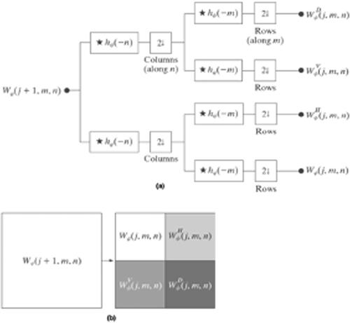
In Figure 9a, assume that the image $f\left(x,y\right)$ is the input to the scale level of j + 1, that is $f\left(x,y\right)=W_{\phi }\left(j+1,m,n\right),$ convolutions of $\star h_{\psi }\left(-n\right)$ and $\star h_{\phi }\left(-n\right)$ are implemented on its rows and downsampling by 2 is applied on its columns, resulting in two sub-images with reduced a horizontal resolution by a factor of 2. Then another step of convolutions is applied on the rows of both sub-images and downsampling is applied on their rows to generate four quarter-size output sub-images, shown in Figure 9b, $W_{\phi }\left(j,m,n\right),$ $W_{\psi }^H\left(j,m,n\right),$ $W_{\psi }^V\left(j,m,n\right)$ and $W_{\psi }^D\left(j,m,n\right).$ If we iterate decomposition for more levels, the approximation coefficients $W\phi \left(j,m,n\right)$ is the input of the next level of decomposition.

The image feature vector is often built with the Frobenius norm of three detail coefficients, that is, ${\left|\left|W_{\psi }^i\left(j,m,n\right)\right|\right|}_F$ where $i=\left\{H,V,D\right\}.$ Frobenius norm is denoted by ${\left|\left|·\right|\right|}_F$ (Strang 2007). For instance, the Frobenius norm of $X$ is ${\left|\left|X\right|\right|}_F=\sqrt{{\sum }_{i=1}^n{\sum }_{j=1}^n{\left|a_{ij}\right|}^2}.$ The image feature set for our Example 3 is constructed with three elements by taking the Frobenius norm for detail coefficients of level 1.

References

- Abbasi, S. A. 2010. On the performance of the EWMA chart in the presence of two-component measurement error. Quality Engineering 22 (3):199–213. doi: 10.1080/08982111003785649.
- Ahonen, T., A. Hadid, and M. Pietikainen. 2006. Face description with local binary patterns: Application to face recognition. IEEE Transactions on Pattern Analysis and Machine Intelligence 28 (12):2037–41. doi: 10.1109/tpami.2006.244.
- Allen, T. T. 2019. Introduction to engineering statistics and lean six sigma: Statistical quality control and design of experiments and systems, vol. 3. London: Springer.
- Allen, T. T., Z. Sui, and K. Akbari. 2018. Exploratory text data analysis for quality hypothesis generation. Quality Engineering 30 (4):701–12. doi: 10.1080/08982112.2018.1481216.
- Allen, T. T., H. Xiong, and S.-H. Tseng. 2020. Expert refined topic models to edit topic clusters in image analysis applied to welding engineering. Informatics 7 (3):21. doi: 10.3390/informatics7030021.
- Bisgaard, S. 1996. The importance of graphics in problem solving and detective work. Quality Engineering 9 (1):157–62. doi: 10.1080/08982119608919028.
- Blei, D. M., A. Y. Ng, and M. I. Jordan. 2003. Latent Dirichlet allocation. Journal of Machine Learning Research 3:993–1022. doi: 10.1162/jmlr.2003.3.4-5.993.
- Canny, J. 1986. A computational approach to edge detection. IEEE Transactions on Pattern Analysis and Machine Intelligence PAMI-8 (6):679–98. doi: 10.1109/TPAMI.1986.4767851.
- Chang, S. I., and J. S. Ravathur. 2005. Computer vision based non-contact surface roughness assessment using wavelet transform and response surface methodology. Quality Engineering 17 (3):435–51. doi: 10.1081/QEN-200059881.
- Chen, J., S. Shan, C. He, G. Zhao, M. Pietikäinen, X. Chen, and W. Gao. 2009. WLD: A robust local image descriptor. IEEE Transactions on Pattern Analysis and Machine Intelligence 32 (9):1705–20. doi: 10.1109/tpami.2009.155.
- De Mast, J., and M. Bergman. 2006. Hypothesis generation in quality improvement projects: Approaches for exploratory studies. Quality and Reliability Engineering International 22 (7):839–50. doi: 10.1002/qre.767.
- De Mast, J., S. H. Steiner, W. P. Nuijten, and D. Kapitan. 2023. Analytical problem solving based on causal, correlational and deductive models. The American Statistician 77 (1):51–61. doi: 10.1080/00031305.2021.2023633.
- De Mast, J., and A. Trip. 2007. Exploratory data analysis in quality-improvement projects. Journal of Quality Technology 39 (4):301–11. doi: 10.1080/00224065.2007.11917697.
- Ghorai, S., A. Mukherjee, M. Gangadaran, and P. K. Dutta. 2013. Automatic defect detection on hot-rolled flat steel products. IEEE Transactions on Instrumentation and Measurement 62 (3):612–21. doi: 10.1109/TIM.2012.2218677.
- Gonzalez, R. C., and R. E. Woods. 2018. Digital image processing. 4th ed. Bangalore, India: Pearson Education.
- Good, I. J. 1983. The philosophy of exploratory data analysis. Philosophy of Science 50 (2):283–95. doi: 10.1086/289110.
- Griffiths, T. L., and M. Steyvers. 2004. Finding scientific topics. Proceedings of the National Academy of Sciences of the United States of America 101 (Suppl 1):5228–35. doi: 10.1073/pnas.0307752101.
- Harris, C., and M. Stephens. 1998. A combined corner and edge detector. Paper presented at the Proceedings of 4th Alvey Vision Conference, Manchester, UK, August 31–September 2.
- Hoaglin, D. C., F. Mosteller, and J. W. Tukey. 1983. Understanding robust and exploratory data analysis. New York, NY: Wiley.
- Lawson, J. 2019. Phase II monitoring of variability using Cusum and EWMA charts with individual observations. Quality Engineering 31 (3):417–29. doi: 10.1080/08982112.2018.1557205.
- Lepenioti, K., A. Bousdekis, D. Apostolou, and G. Mentzas. 2020. Prescriptive analytics: Literature review and research challenges. International Journal of Information Management 50:57–70. doi: 10.1016/j.ijinfomgt.2019.04.003.
- Lucas, J. M., and M. S. Saccucci. 1990. Exponentially weighted moving average control schemes: Properties and enhancements. Technometrics 32 (1):1–12. doi: 10.1080/00401706.1990.10484583.
- Nederbragt, A. J., P. Francus, J. Bollmann, and M. J. Soreghan. 2005. Image calibration, filtering, and processing. In Image analysis, sediments and paleoenvironments, ed. P. Francus, 35–58. Dordrecht: Springer. doi: 10.1007/1-4020-2122-4_3.
- Niiniluoto, I. 1999. Defending abduction. Philosophy of Science 66 (S3):S436–S451. doi: 10.1086/392744.
- Qiu, P. 2018. Jump regression, image processing, and quality control. Quality Engineering 30 (1):137–53. doi: 10.1080/08982112.2017.1357077.
- Reddy, G. P. O. 2018. Digital image processing: Principles and applications. In Geospatial technologies in land resources mapping, monitoring and management. Geotechnologies and the environment, eds. G. P. O. Reddy and S. K. Singh, vol 21, 1–30. Cham: Springer. doi: 10.1007/978-3-319-78711-4_6.
- Roberts, S. W. 1959. Control chart tests based on geometric moving averages. Technometrics 1 (3):239–50. doi: 10.1080/00401706.1959.10489860.
- Robinson, T. J., R. C. Giles, and R. U. Rajapakshage. 2020. Discussion of “Experiences with big data: Accounts from a data scientist’s perspective. Quality Engineering 32 (4):543–9. doi: 10.1080/08982112.2020.1758333.
- Rong, W., Z. Li, W. Zhang, and L. Sun. 2014. An improved Canny edge detection algorithm. IEEE International Conference on Mechatronics and Automation, Tianjin, China, August 3–6, 577–582. doi: 10.1109/ICMA.2014.6885761.
- Rosen-Zvi, M., C. Chemudugunta, T. Griffiths, P. Smyth, and M. Steyvers. 2010. Learning author-topic models from text corpora. ACM Transactions on Information Systems 28 (1):1–38. doi: 10.1145/1658377.1658381.
- Rosten, E., and T. Drummond. 2006. Machine learning for high-speed corner detection. Paper presented at the Proceedings of 9th European Conference on Computer Vision, Graz, Austria, May 7–13, vol. 2, 430–43.
- Shewhart, W. A. 1931. Economic control of quality of manufactured product. Princeton, NJ: Van Nostrand Reinhold. doi: 10.2307/2277676.
- Shewhart, W. A. 1939. Statistical method from the viewpoint of quality control. Washington, DC: Department of Agriculture, The Graduate School USA. (Reprint 1986; New York, NY: Dover Publications.)
- Strang, G. 2007. Linear algebra and its applications. 4th ed. Hoboken, NJ: Nelson Engineering.
- Teh, Y. W., D. Newman, and M. Welling. 2007. A collapsed variational Bayesian inference algorithm for latent Dirichlet allocation. In Advances in neural information processing systems, eds. B. Schölkopf, J. Platt and T. Hoffman, 1353–60. Vancouver, CA: MIT Press.
- Tsai, R. Y. 1987. A versatile camera calibration technique for high accuracy 3D machine vision metrology using off-the-shelf TV cameras and lenses. IEEE Journal on Robotics and Automation 3 (4):323–44. doi: 10.1109/JRA.1987.1087109.
- Tukey, J. W. 1977. Exploratory data analysis. Reading, PA: Addison-Wesley.
- Vining, G., M. Kulahci, and S. Pedersen. 2016. Recent advances and future directions for quality engineering. Quality and Reliability Engineering International 32 (3):863–75. doi: 10.1002/qre.1797.
- Wu, Z., M. Xie, and S. Zhang. 2005. A virtual system for vision based SPC. Quality Engineering 17 (3):337–43. doi: 10.1081/QEN-200059835.
- Zhang, Z. 2000. A flexible new technique for camera calibration. IEEE Transactions on Pattern Analysis and Machine Intelligence 22 (11):1330–4. doi: 10.1109/34.888718.