Simulating water balance and evapotranspiration in a subsurface drained clayey agricultural field in high-latitude conditions

Abstract

Secondary drainage impact of groundwater outflow can affect drainage design and form a pathway for nutrient loading in agricultural areas. Holistic assessment of water balance and all outflow pathways can benefit design of sustainable drainage in a changing climate. In this study, three-dimensional, hydrological FLUSH model was applied to investigate a field-scale data set and to produce a closure of water balance throughout all seasons in a clayey subsurface drained agricultural field in high-latitude conditions. Description of evapotranspiration (ET)-groundwater interactions using a three-dimensional hydrological model provides a new approach for evaluating standard computational methods to estimate ET with limited crop data. Different ET estimates were tested in the context of total water balance, and the coupling of ET and groundwater outflow was assessed. Comparison of measured and simulated water balance components demonstrated that reference ET (Penman–Monteith method) overestimated ET in the cropped field in high latitude conditions. The FAO-56 single crop coefficient approach was also noted to overestimate ET in the studied conditions. A calibrated constant crop coefficient satisfactorily described ET in spring and in autumn, but underestimated it during summer periods. The results suggest that care should be taken when applying standard methods in high-latitude conditions. Groundwater outflow and ET were shown to be interlinked, but even a relatively high potential ET affected the amount of groundwater outflow only slightly. The results demonstrate that groundwater outflow can form an important component of the water balance in clayey subsurface drained fields. The strength of the 3D model was demonstrated in showing how ET had an impact on all outflow components of drained field sections. Such a modelling tool is useful for generating scenarios that show how changes in climate forcing and thereby ET can alter the partitioning of the field-scale water balance.

Keywords:

• water balance
• groundwater outflow
• crop evapotranspiration
• drainage
• 3D modeling
• structured soil

1. Introduction

Water flow pathways and hydrological processes can notably affect nutrient loads from agricultural fields to surface waters (e.g. Turtola & Paajanen 1995; Vagstad et al. 2004). Outflow pathways in agricultural fields are commonly assessed by measurements of surface runoff and drain discharge quantity and quality. Also flow of water in open ditches or in channels can be measured with standard methods, but lateral seepage of water through the field boundaries below the drainage systems (hereby called groundwater outflow) has been rarely quantified. Recent studies have shown that groundwater outflow can be an important component of water balance (Rozemeijer et al. 2010; Turunen et al. 2013) and nutrient loading (Rozemeijer & Broers 2007; Rozemeijer et al. 2010). However, its contribution in high-latitude conditions is understudied. Therefore, it would be necessary to conduct a holistic assessment of water balances of arable areas in boreal climatic conditions and clayey structured soils, which are common in Nordic-Baltic regions (e.g. Vagstad et al. 2004). Also, since climate change can notably affect the hydrology of the regions (e.g. Veijalainen et al. 2010) and the nutrient loading from arable areas (Puustinen et al. 2007), it would be beneficial to have computational tools for the design of effective and sustainable drainage in the changing conditions.

Quantification of all water balance components, especially evapotranspiration (ET) and groundwater outflow, through measurements is challenging. Hydrological model applications provide one method to quantify the missing components and close the water balance. However, catchment-scale water balance modeling studies are practically unable to determine all flow components without internal catchment data (Gallart et al. 2007). Field-scale water balance and solute transport studies based on modeling approaches are often conducted with 1D models (e.g. Larsson & Jarvis 1999) or conceptual models (e.g. Knisel & Turtola 2000) which simplify or exclude lateral flow processes. Hydrological effects of lateral flow components have been noticed in several studies in agricultural fields with structured soil (e.g. Larsson & Jarvis 1999; Gärdenäs et al. 2006; Hintikka et al. 2008), but the contribution of groundwater outflow to the total water balance has been rarely assessed. Turunen et al. (2013) and Warsta, Karvonen, et al. (2013, Warsta et al. 2014) simulated the hydrology of clayey agricultural fields in southern Finland with the 3D FLUSH model (Warsta 2011; Warsta, Karvonen, et al. 2013). They showed that groundwater outflow can be an important component of the water balance during snow- and frost-free periods, but did not assess long-term water balance through all seasons. Turunen et al. (2013) and Warsta, Karvonen, et al. (2013) used a relatively simple method to estimate ET, and assumed potential ET from cropped surface in high latitude conditions to be notably lower than the reference ET (Penman–Monteith method) suggested by Allen et al. (1998). Reference ET represents potential ET from a grass surface which has specific and constant crop characteristics such as albedo, height and surface resistance (Allen et al. 1998). The assumption of Turunen et al. (2013) and Warsta, Karvonen, et al. (2013) is plausible when, e.g. bare soil and sprouts induce notably less ET than a grass surface. However, in certain conditions, bare soil evaporation can be higher than the reference ET (Lewan 1993). Underestimation of ET may lead to a biased estimate of the simulated amount of groundwater outflow as ET and groundwater outflow are interlinked in the simulations. Since ET is typically the largest component of the annual water balance in agricultural fields in high-latitude conditions, there is a need to evaluate different methods to estimate crop ET in high latitudes.

In this study the FLUSH model, coupled with wintertime process descriptions (Koivusalo et al. 2001; Warsta et al. 2012), is applied with a data set presented by Vakkilainen et al. (2008, 2010) and Äijö et al. (2014) in a clayey agricultural field in southern Finland to (1) quantify the contribution of groundwater outflow in the year-round water balance, (2) test the capability of the reference ET and FAO-56 approach (Allen et al. 1998) for describing ET in cropped areas in high-latitude conditions and (3) assess the effects of different ET estimates on the water balance and outflow components. By simulating the water balance with different ET estimates we attempted to quantify the ranges where ET and groundwater outflow must reside.

2. Materials and methods

2.1. Site and measurements

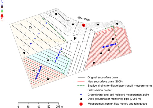
The study site is an agricultural field located in Jokioinen, southern Finland (60° 51′59ʺN, 23° 25′ 50ʺE). The field is subsurface drained, and the soil has a high clay content of 66–88%. Top soil of 0–0.2 m has a clay content of 66–67% and a soil organic matter content of 5.7–7.2%. The soil is classified as Vertic Luvic Stagnosol (FAO 2007) and similar soil is described in detail by Yli-Halla et al. (2009). The field has been cultivated for decades, and spring barley (Hordeum vulgare) and oats (Avena sativa) were cultivated during the current study period. The area was divided into four monitored field sections (Sections A–D, Figure 1) to assess the hydrology of the field sections with different drainage systems (Vakkilainen et al. 2010; Turunen et al. 2013; Äijö et al. 2014). The monitored field sections have a mean slope of <1%, although a steep slope is located in the northern side of the field, as shown in Figure 1. Sections B (1.3 ha) and D (3.4 ha) have relatively wide drain spacings of 16 m and 32 m, respectively. Sections A (2.9 ha) and C (1.7 ha) have denser drain spacings of 6 m and 8 m, respectively. Sections B, C and D have an average drain depth of 1.0 m, and Section A 0.9 m. All the drains have an inner diameter of 0.05 m. Unmonitored field section E (5.6 ha, Figure 1) was included in the simulations to facilitate modeling of the entire field. Finnish subsurface drainage design guidelines in 1980s (Saavalainen 1984) recommended a drain spacing of 14–16 m and a depth of 1 m for clayey soils in southern Finland. Later, the recommendation for Finnish clayey soils has changed to the spacing of 10–14 m and the depth of 1 m (Paasonen-Kivekäs et al. 2009). Thus, the drainage design of the studied field (excluding Section D) is close to the typical drainage systems of clayey agricultural fields in southern Finland.

Figure 1. Drainage networks and measurement devices in the Nummela Experimental Field (Turunen et al. 2013).

Drain discharge and tillage layer runoff were measured automatically with a time resolution of 15 min with Datawater WS Vertical helix meter (Maddalena, Povoletto, Italy). Tillage layer runoff was collected with shallow subsurface drains at the depth of 0.4 m, and these drains had coarse gravel as trench backfill. Hence, tillage layer runoff measurements represent both surface runoff and subsurface flow in the tillage layer. Level of the groundwater table (LGT) was measured weekly or bi-weekly in the middle of the drain lines (Figure 1) with plastic groundwater observation tubes (bottom closed, perforated). In heavy clayey soils, it is unclear whether the LGT measurements actually describe water table in soil matrix or soil macropore system. We hypothesize that measured LGT describes either one of the systems, or their combination, depending on how the monitoring tube is located in relation to the macropore network. Flow measurements from the drainage systems described earlier were conducted continuously from June 2008 to December 2013. A malfunction afflicted the tillage layer runoff measurements during autumn 2008 in Section B, and tillage layer runoff was not measured during this time period in the section. Also, it was observed that during spring snowmelt, the shallow drains gathering tillage layer runoff in Section B received waters outside of the section, and therefore, the amount of tillage layer runoff was overestimated from the Section B during spring periods. Snow water equivalent (SWE) was measured weekly or bi-weekly based on weighed snow samples. However, in 2008–2009, only snow depth was measured. SWE during this time period was estimated as a function of snow depth and long-term average snow density.

Water retention curves (WRC) and volumetric fraction of macropores (defined as pores which empty at the suction of 0.1 m) were measured from three soil layers (0.0 –0.2 m, 0.2–0.4 m and 0.4–0.6 m) from soil samples having a diameter of 150 mm. WRCs were measured at the pressures of 0 m, −0.1 m, −1.0 m and −150.0 m as a drying curve.

Precipitation was measured on site with a RAINEW 111 tipping bucket rain gauge (RainWise Inc., Bar Harbor, ME, USA) with the time resolution of 15 min. The measured precipitation was corrected with coefficients of 1.05 and 1.3 for rainfall and snowfall, respectively, following Førland et al. (1996). Other meteorological data were measured at the Jokioinen Observatory (7 km from the Nummela Field) administrated by the Finnish Meteorological Institute. Intermittently missing data (approximately 2%) were replaced with data from the observatory of the Finnish Meteorological Institute at the Helsinki-Vantaa Airport (105 km from the Nummela Field). Daily Class A pan evaporation measurements were conducted from the beginning of May to October or November at the Jokioinen Observatory by the Finnish Environment Institute.

The measurements and the data sets are presented in more detail in Turunen et al. (2013), Vakkilainen et al. (2008, 2010) and Äijö et al. (2014).

2.2. FLUSH

FLUSH is a 3D process-based model tailored for simulating water balance and environmental loads in clayey agricultural fields (Warsta 2011; Turunen et al. 2013; Warsta, Karvonen, et al. 2013, Warsta, Taskinen, 2013; Salo et al. 2014). The simulated area is divided into overland and subsurface domains. Overland flow is computed in 2D with the diffuse wave approximations of the Saint Venant equations. The soil pore space is divided into mobile matrix and macropore systems. The dual-permeability approach is applied to describe aggregated soils such as clay and enables simulation of slow water movement in the soil matrix and fast preferential flow in macropores. Soil macropores are composed of static and dynamic macropores. Static macropores represent permanent preferential flowpaths, such as biopores and structural cracks, while dynamic macropores represent shrinkage cracks. The swelling and shrinkage component of the model is derived from the SWAP model (van Dam et al. 2008). Simulation of subsurface water flow is based on the Richards' equation and van Genuchten (1980) schemes in both pore systems.

The model can simulate as many open ditches and subsurface drainage systems as necessary (Turunen et al. 2013). Each drain and ditch element can be parameterised separately, and they are treated as cell internal sinks in the model. Lateral groundwater outflow removes water from the horizontally outermost grid cells, and the flux is calculated with the Darcy's law. The hydraulic head gradient is calculated as the elevation difference between the outermost grid cell and the corresponding grid cell outside the field boundary. Bottom of the field is considered impermeable in the simulations. Flow to subsurface drains is also calculated with the Darcy's law, but the distance variable is replaced with a calibrated entrance parameter, which can be interpreted as an equivalent flow path length.

Potential ET (PET) is given as a pre-computed input time series, and actual ET is calculated by reducing PET in dry and wet soil moisture conditions following Feddes et al. (1978). PET is distributed vertically to the soil profile according to the root mass distribution, which is set to linearly decrease between soil surface and prevailing root depth. The root depth can be changed during the simulation to describe root development and crop harvest in the autumn.

Wintertime processes were recently added to the model. Snow accumulation and melt are simulated with the process-based model of Koivusalo et al. (2001). Freezing and thawing processes are computed with a modified convection-diffusion equation, as described in Warsta et al. (2012). Phase transitions of water consume or release energy in the model, while convection and conduction transport heat in the soil profile. Currently, soil freezing does not affect flow of water in the model.

In the model, precipitation is initially stored in the depression storage on the field surface where it can infiltrate into the soil matrix and macropores. Depth of the depression storage can be set to vary with time, e.g. to account for the soil tillage impact on the depression storage. Horizontal overland flow occurs when the level of the groundwater table rises to the soil surface or when soil infiltration capacity is exceeded and the depression storage is full. ET, open ditches, subsurface drains and lateral groundwater outflow remove water from the simulated domain.

2.3. Evapotranspiration

Three different PET schemes were tested in the model application. Two schemes are based on the Penman–Monteith method (Allen et al. 1998) and one on the Class A pan measurements. The method of Allen et al. (1998) is also called FAO-56 approach, and it provides ET estimation methods for reference and cropped surfaces. Class A evaporation pan measurements combined with pan coefficients or adjustment functions are widely used to estimate ET (e.g. McMahon et al. 2013). Class A pan is constructed of galvanised iron, and it has a diameter of 1.2 m and depth of 0.25 m. The pan is placed 30–50 mm above the ground on a wooden structure and filled with water to observe evaporation-induced changes in the water level.

In the schemes based on the Penman–Monteith method, reference PET (PET0) for a grass reference surface having specific characteristics was computed as described in Allen et al. (1998). The meteorological input for PET0 estimation was calculated similarly as Turunen et al. (2013), but hourly cloudless time was computed by dividing sum of measured short-wave radiation of the closest 24 h by the corresponding estimated clear-sky short-wave radiation. Clear-sky short-wave radiation was computed as a function of location, following Allen et al. (1998). PET0 was set to 0 when air temperature was below the freezing point. The snow model simulates winter evaporation from the surface of the snow pack with an energy balance based approach (Koivusalo et al. 2001).

Since cropped soil surfaces differ essentially from the grass reference surface, potential crop ET had to be estimated. Cropped surfaces have time-dependent and essentially different characteristics (crop height, albedo, surface resistance and evaporation from soil) than the grass reference surface. Potential crop ET is in this study calculated by multiplying PET0 with a crop coefficient, which represents the changes in the characteristic of the surface. Crop coefficient can vary temporally according to the growing stage. Potential ET describes the ET rate from a surface which is not limited by the availability of water in the root zone. Actual ET is calculated in FLUSH by reducing the PET according to the prevailing soil moisture conditions in the root zone (see Section 2.2).

Potential crop ET was computed with two approaches. First, a constant crop coefficient of 0.7 was adopted from the water balance study of Turunen et al. (2013) (PET07). Second, crop coefficients were estimated with the single crop coefficient method of Allen et al. (1998) (PETCropc). Since Allen et al. (1998) did not present the duration of growing season phases in a boreal climate, duration of the stages were calculated on the basis of effective degree days (EDD). The growing season was divided into initial, development, mid-season, late-season and end-stage phases. EDD needed for each stage were 150 EDD from sowing to the end of the initial phase, 350 EDD for the development phase and 450 EDD for the mid-season phase (Peltonen-Sainio & Rajala 2008). The late-season phase was set to last from the end of mid-season phase to the harvest date. The end-stage was set to prevail after the late-season phase. Corresponding crop coefficients were calculated for each of the phases. Allen et al. (1998) recommended calculating the initial phase crop coefficient as a function of soil properties and daily meteorological data, and applying the same method for bare soil conditions. Initial phase coefficient was calculated in spring with the data from 1 May (but sowing date was used if it was earlier) to the end of the phase. The maximum cumulative amount of water that can evaporate from bare or nearly bare wet soil with energy-limited evaporation rate (before portion of evaporation occurs beneath soil surface) was set to 6 mm following Ritchie (1972). Moisture contents at the wilting point and field capacity were adapted from the measurements. Other parameters were set as recommended by Allen et al. (1998). End-phase crop coefficient was calculated similarly as the initial phase coefficient, but with the meteorological data from the harvest date to 1 October. After initial stage, the crop coefficient was set to linearly increase to the mid-season crop coefficient. Mid-season crop coefficient for the local conditions was initially set to 1.15 and then adjusted as a function of meteorological data and plant height (Allen et al. 1998). Plant height during this phase was set to 0.8 m. As suggested by Allen et al. (1998), after mid-season phase, the crop coefficient was set to linearly decrease to the end-stage crop coefficient value.

The third method to estimate PET was based on the Class A measurements (PETClassA). First, the daily Class A measurements were corrected to local conditions with the equation of Vakkilainen (1982):

(1)

where C is the correction coefficient (from 1 May), J is Julian day and d is 121 in leap years and 120 in regular years. Vakkilainen (1982) derived the function empirically by comparing measured ET from grass-covered lysimeters to Class A data, and it thus represents reference ET conditions. Vakkilainen (1982) also simulated ET and energy balance in the lysimeters with an extended Penman method and reported average bi-hourly distribution of energy consumed by ET within a day during different periods of growing season. In the current study, the corrected daily Class A ET estimate was disaggregated to hourly values by multiplying the daily value with the corresponding bi-hourly fraction and dividing it by two.

To compare the PET estimates to crop PET estimates of other models, crop PET was also calculated with the MACRO model (e.g. Jarvis and Larsbo 2012). Crop PET was calculated with the default values of MACRO using daily meteorological data and sowing as well as harvest dates as input values.

2.4. Model set up

The parameterisation of the field was partly derived from Turunen et al. (2013), but in this study, the description of the soil hydraulic parameters were improved, and the model was recalibrated. Calibration was conducted against drain discharge, tillage layer runoff and LGT for the time period 1 January 2011–31 December 2011 with PET07. The model was validated against the corresponding data from 6 May 2008–31 December 2009. The whole field was simulated as a single domain. Results were analysed from two hydrologically different (different drain spacing, soil hydraulic properties and topography) field Sections (B and D) to assess the role of ET in their water balance. Section B represents a field section with typical subsurface drainage system of a clayey agricultural field in southern Finland, and Section D a field section with a larger drain spacing and higher soil moisture conditions.

Horizontal cell size in the computational grid was set to 5 m × 5 m, and the vertical grid profile (depth 2.4 m) was divided into 16 cells with the depths ranging from 0.02 m to 0.5 m (Turunen et al. 2013). The grid boundaries were set according to the monitored field area (Figure 1), but at the north-east side of the field, the grid boundaries were retracted approximately 5 m towards the field area from the center of the main ditch.

Turunen et al. (2013) calibrated macroporosity of the subsoil (depth >1.05 m) for each field section, but in this study, a single value was calibrated to describe the volumetric fraction of macropores in the subsoil of the entire field. The calibrated value was 0.07%. This approach can be considered to provide a more plausible description of the field hydrology, since Turunen et al. (2013) applied relatively high macroporosity values in the subsoil of Section E. In addition, Berisso et al. (2013), who measured pore characteristic in a clayey soil in Jokioinen, noticed that air permeability was anisotropic especially close to the soil surface. Following Berisso et al. (2013), the ratio of lateral to vertical saturated hydraulic conductivity in the macropores was set to 0.02 in the soil layers at the depth of 0–0.425 m, 0.83 at the depth of 0.425–1.05 m and to 1 below this depth. The saturated hydraulic conductivity of the soil matrix was assumed to be isotropic in all soil layers. Due to these changes, the drain entrance parameter, which can be interpreted as the equivalent flow path length (see Turunen et al. 2013, Eq. 4), was calibrated to values of 5 m and 7 m in Sections B and D, respectively.

Turunen et al. (2013) adapted soil water retention data for the dry end of the WRCs from the Hovi experimental field (e.g. Warsta et al. 2014). In the current study, measurements of the soil water content at the wilting point were available, and therefore, WRCs were recalculated with complete water retention data set from the Nummela Field with the hydraulic pressure head values of 0.0 m, −0.1 m, −1.0 m and −150.0 m. The parametric WRCs for different soil layers are listed in Table 1. The unmonitored Section E was parameterised similarly as Section A.

Table 1. Parameters for the water retention curves derived by fitting the van Genuchten (1980) model to the measured values. Sections A to D as in Figure 1.

Parameters	Section A, 0.0–0.25 m	Section B, 0.0–0.25 m	Section C, 0.0–0.25 m	Section D, 0.0–0.25 m
α [m^−1]	2.008	2.548	2.886	3.561
c [–]	1.150	1.145	1.149	1.147
θr [m^3 m^–3]	0.100	0.100	0.100	0.010
θs [m^3 m^–3]	0.529	0.543	0.529	0.560
Parameters	Section A, 0.25–0.45 m	Section B, 0.25–0.45 m	Section C, 0.25–0.45 m	Section D, 0.25–0.45 m
α [m^−1]	0.437	0.273	0.412	0.333
c [–]	1.106	1.150	1.161	1.145
θr [m^3 m^−3]	0.100	0.100	0.100	0.100
θs [m^3 m^−3]	0.554	0.551	0.539	0.555
Parameters	Section A, 0.45–2.4 m	Section B, 0.45–2.4 m	Section C, 0.45–2.4 m	Section D, 0.45–2.4 m
α [m^−1]	0.678	1.072	0.679	0.576
c [–]	1.104	1.095	1.127	1.115
θr [m^3 m^−3]	0.100	0.100	0.100	0.100
θs [m^3 m^−3]	0.602	0.591	0.534	0.579

α = parameter of the van Genuchten (1980) model.

c = parameter of the van Genuchten (1980) model.

θ_r = residual water content.

θ_s = saturated water content.

The critical pressure heads for the soil moisture limits of Feddes et al. (1978) were set to −150.0 m for the wilting point, −5 m for the critical dry-end pressure head, and −0.1 m for the critical wet-end pressure head, following Vakkilainen (1982) and Warsta, Karvonen, et al. (2013). Root maximum depth was set to 0.8 m (Turunen et al. 2013), which is in the range (0.35–0.8 m) of maximum root depths in Finnish clay soils reported by Ilola et al. (1988). Root depth was set to linearly increase from the minimum (0.05 m) to the maximum depth during the time period from sowing to 3 June (Turunen et al. 2013). Root depth was set back to the minimum value at the time of harvest.

The model results were evaluated with the modified Nash–Sutcliffe (NS) model efficiency coefficient and the mean absolute error (MAE) following Legates and McCabe (1999).

3. Results

3.1. Model calibration and validation

Cumulative corrected precipitation during the calibration period (2011) was 676 mm. Other simulated components of the water balance in the whole field area (Sections A-E) were ET (48% of precipitation), drain discharge (20% of precipitation), flow to open ditches (18% of precipitation), groundwater outflow (15% of precipitation) and storage change (7% of precipitation). The flow to open ditches component includes both overland flow and seepage to all simulated open ditches. Clearly, most of the flow to open ditches occurred as seepage to the ditches surrounding the field. According to the measurements, the ratio of drain discharge to tillage layer runoff in the monitored field sections (excluding Section B due to the measurement problem) was 2.25, though in Section D the ratio was 0.63.

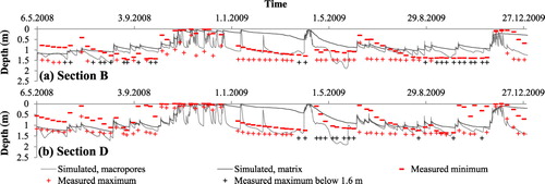
NS values of 0.56 and 0.44 for the hourly drain discharge in Sections B and D, respectively, indicate a satisfactory fit against the measured drain discharge. Difficulties with the simulation of the spring snowmelt caused the relatively low NS value for the drain discharge in Section D, and the value was 0.62 when the discharge during snowmelt was excluded. Cumulative simulated drain discharges corresponded with the measured values with the bias of 22 mm and 24 mm from 1 January to 31 December in Sections B and D, respectively. The simulated tillage layer runoff compared to the measured values similarly as in the study of Turunen et al. (2013), i.e. hourly NS values were poor, but the modelled cumulative values were close to the measured values, except during spring snowmelt (Figure 2a–b). The difference during spring snowmelt in Section B was caused by surface runoff entering the section from the surrounding field sections. The measured values do, therefore, not properly represent the amount of tillage layer runoff from the Section B and are not shown. The measured total tillage layer runoff was also clearly higher than the maximum annual SWE and precipitation during the spring melt period which again indicates that the data during this time period do not represent runoff from Section B. The difference between the cumulative measured and simulated tillage layer runoff was −15 mm in Section B in autumn 2011, and 27 mm in Section D in January–December 2011. The model was able to simulate SWE with the MAE value of 6 mm, and the timing of the spring snowmelts corresponded well with the outflow measurements, as shown in Figure 2a–b. Clearly, most of the outflow from the field section occurred in the spring and the autumn. The amount of actual ET during the simulation period was 306 mm, which is close to the PET07 value of 330 mm.

Figure 2. Simulated and measured snow water equivalent (SWE), and cumulative simulated and measured drain discharge and tillage layer runoff in field Sections (a) B and (b) D in the calibration period 1 January–31 December 2011.

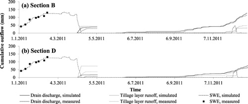
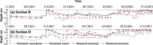
The simulated LGTs in the soil matrix or in the macropores were between the measured maximum and minimum LGT values during most of the simulation period (Figure 3a–b), excluding August and beginning of September 2011, when the simulated LGTs were clearly higher compared to the measured values, especially in Section B. Also, the simulated LGTs rose more slowly to the field surface compared to the measured levels in autumn 2011.

Figure 3. Average simulated groundwater table levels in soil macropores and matrix, and measured minimum and maximum depths in field Sections (a) B and (b) D in calibration period 1 January–31 December 2011.

During the validation period (May 2008 to December 2009) cumulative corrected precipitation was 1023 mm. ET was 55%, drain discharge 15%, flow to open ditches 10%, groundwater outflow 15% and storage change 6% of precipitation.

NS values of drain discharge during the validation period were comparable to the calibration period with values of 0.51 and 0.38 in Sections B and D, respectively. The simulated and measured cumulative drain discharge values corresponded well with each other in autumn 2008 (bias values of 1 mm and 10 mm in Sections B and D, respectively) and 2009 (bias values of −5 mm and −10 mm in Sections B and D, respectively). The model overestimated most of the outflow events in spring 2009 probably partly due to the slightly inaccurate amount and timing of maximum SWE during the winter (Figure 4a–b). However, during spring 2009, the timing of the drain discharge and runoff events corresponded well with the measurements.

Figure 4. Simulated and measured snow water equivalent (SWE), cumulative simulated and measured drain discharge and tillage layer runoff in field Sections (a) B and (b) D in validation period 6 May 2008–31 December 2009.

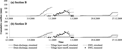
In Section B, the tillage layer runoff measurement system did not function in autumn 2008. In spring 2009, the simulated amount of tillage layer runoff in the section was notably lower than the measured value due to the similar measurement problems as in spring 2011 (Figure 4a). In autumn 2009, both simulated and measured tillage layer runoff values were close to 0 mm in Section B. In Section D, the simulated cumulative tillage layer runoff was notably higher than the measured values in autumn 2008 (22 mm) and spring 2009 (32 mm) (Figure 4b). During autumn 2009 the model underestimated the amount of tillage layer runoff by 15 mm in the section.

Simulated LGT during the model validation corresponded with the measured values similarly as during the calibration period (Figure 5a–b). Most of the time the simulated levels were between the measured minimum and maximum values, excluding the periods in August and early September when the simulated values were typically higher than the measured values.

Figure 5. Average simulated groundwater table levels in soil macropores and matrix, and measured minimum and maximum depths in field Sections (a) B and (b) D in validation period 6 May 2008–31 December 2009.

3.2. ET scenarios

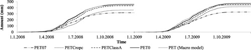
The simulations were run with three different ET estimates. PETClassA and PET0 estimates resembled each other closely, and accumulated PETClassA was only 3% lower than accumulated PET0 (sums from 2008 to 2009 and 2011, from May to December). Class A measurements were only available annually from 1 May, and therefore, measurements before this date were replaced with PET0 estimates.

PETClassA resulted in the highest annual ET of the ET models tested in the simulations, PETCropc resulted in clearly lower values than PETClassA, and PET07 gave the lowest estimate (Figure 6). Also, crop PET calculated with the MACRO model with daily meteorological data closely resembled our PET0 estimate (Figure 6).

Figure 6. Cumulative PET computed with different methods in 1 January 2008–31 December 2009.

As shown in Figure 7a–d, the magnitude of PET notably affects the outflow components of the studied fields. When PETCropc or PETClassA was used as a model input, the autumn drain discharge events occurred later (2008 and 2011) or were notably smaller (2009) than the measured values. PET estimate did not essentially affect tillage layer runoff events during spring periods, but in autumn periods, the lowest PET estimate resulted into higher amount of tillage layer runoff, especially in Section D. Overestimation of the simulated tillage layer runoff during autumn periods in model calibration and validation in Section D is likely due to a too low estimate of ET during the late growing season or autumn.

Figure 7. Cumulative simulated drain discharge and tillage layer runoff with different ET scenarios in Sections (a) B and (b) D in 1 January–31 December 2011 as well as (c) B and (d) D in 6 May 2008–31 December 2009.

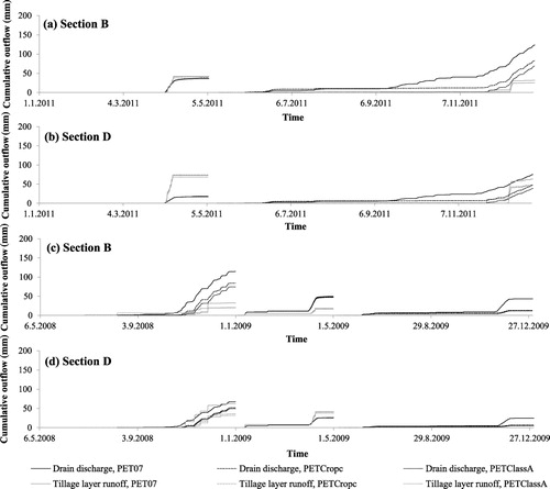
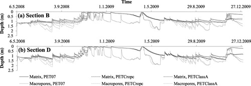
The magnitude of the PET estimate also affected the level of the groundwater table in both of the studied field sections, especially in autumn and in summer periods (Figure 8a–b). As shown in Figures 3a–b and 5a–b, PET07 estimate was too low during summer periods. Higher PET estimate performed better during the studied summer periods. However, both PETCropc and PETClassA estimates resulted in too low simulated groundwater table levels in autumn periods.

Figure 8. Average simulated groundwater table levels in soil macropores and matrix with different ET scenarios in Sections (a) B and (b) D in 6 May 2008–31 December 2009.

Although the accumulations of the different PET estimates in the validation period varied between 595 mm and 818 mm and the actual ET from the soil between 547 mm and 666 mm, the amount of groundwater outflow varied less between 157 mm and 127 mm (Table 2). Groundwater outflow and ET are thus clearly interlinked, but the absolute change in groundwater outflow only partly compensates for the change in ET. As listed in Table 2, higher amount of ET affected clearly more other outflow components, especially drain discharge, than groundwater outflow. This implies that groundwater outflow is more sensitive to the parameterisation of soil properties than the choice of PET estimation method.

Table 2. Components of the simulated water balance [mm] with different PET estimates in the whole field area during the validation period 6 May 2008–31 December 2009.

Scenario	PET07	PETCropc	PETClassA
Precipitation	1023	1023	1023
Potential ET	595	741	818
Actual ET	547	647	666
Evaporation from snow cover	13	13	13
Flow to open ditches	105	83	81
Drain discharge	157	117	108
Groundwater outflow	157	137	127
Change of storage	59	40	42
Mass balance error	−13	−15	−13

Since the model was calibrated with the PET07 estimate, it was also tested if the timing of the simulated drain discharge events would correspond with the measurements with higher PET estimates and different parameterisation of soil properties, i.e. a lower calibrated value for the volumetric fraction of macropores in the soil layers beneath 1.05 m. It was found that even if lateral macropore flow was prevented in the model, the timing of drain discharge events in autumn periods did not correspond with the measured values. This indicates that the timing did not depend on the parameterisation of the deep soil layers and lateral macropore flow, but was clearly more sensitive to the PET estimate. Soil moisture conditions limited the potential ET during validation with 48 (8%) mm, 94 (13%) mm and 152 (19%) mm with PET07, PETCropc and PETClassA estimates, respectively. Actual amounts of simulated ET are listed in Table 2. Simulated evaporation from snow cover and ET during winter was minimal compared to the growing season.

4. Discussion

Different methods to estimate PET notably affected the simulated water balance and outflow components of the studied field sections. Even though ET from bare or nearly bare soil conditions can be as high or even higher than from a grass surface (e.g. Lewan 1993), PET close to PET0 based on the Penman–Monteith method (Allen et al. 1998) was clearly too high in our simulations in high latitude area (61° N). Too high PET estimates resulted in inaccurate timing and low amount of simulated cumulative autumn drain discharge compared to the measurements. Also, when PET was calculated with the crop coefficients for cropped and bare soil conditions following Allen et al. (1998), the timing and amount of cumulative simulated autumn drain discharge did not match with the measurements. The method, however, includes several assumptions and parameters (depth of the evaporative layer, ratio of maximum bare soil evaporation to PET0 and water content available to evaporation), which should be attempted to be calibrated to local conditions (Allen et al. 2005). Our attempts to calibrate these parameters (not shown) did not provide a PET estimate which would have satisfactorily functioned in the water balance model. Also Johnsson and Jansson (1991), who calibrated their ET model against drain discharge data from three plots with different crop cover in central Sweden, noticed that ET from plots where barley was cultivated was notably lower than ET from a grass-covered field plot. Their ET estimates were relatively close to the estimates of our study. On the other hand, Gustafsson et al. (2004) who studied ET from arable areas in central Sweden with eddy flux measurements and ET model simulations reported much higher amount of average annual actual ET (385–434 mm). However, they did not test their ET estimate in a water balance model. They stated that eddy flux measurements involved several uncertainties, e.g. accuracy of latent heat flux measurements was 7.3% and also included systematic error.

Constant crop coefficient of Turunen et al. (2013) functioned well in the model application. However, even though a constant crop coefficient may describe the total amount of ET adequately, it is incapable of describing the temporal differences in ET due to different growing phases of the crops. Also, a more detailed description for ET would require, e.g. a physics-based model for compensatory root water uptake (Jarvis 2011). More detailed physics-based ET models, in turn, would require crop data, and they include parameters, which would have to be calibrated or estimated from literature (e.g. Lewan 1993). Partitioning of ET into different components and taking into account the effects of different stress factors on transpiration (e.g. Lhomme et al. 1998) would be worth studying, e.g. to quantify the effects of cold temperature stress on stomatal resistance and transpiration in arable areas in high latitudes.

PET calculated with the MACRO model was noted to closely resemble the PET0 of the Penman–Monteith method. Even though this PET estimate was noted to be relatively high in the current study, Hintikka et al. (2008) used PET from the MACRO model to study the water balance of a clayey field in conditions similar to the Nummela Field. MACRO was applied to simulate impacts of changing soil properties on water balance in different parts of a sloping field. Based on 1D simulations Hintikka et al. (2008) concluded that a multidimensional model would be required to improve the simulation of the water balance and to take into account lateral flow components in the sloping field. Also, Larsson and Jarvis (1999), who simulated a clayey field plot with the MACRO model noticed an influx of groundwater to the studied site. Larsson and Jarvis (1999) did not take this into account in the model, but divided the measured drain discharge by the ratio of discharge in the studied plot and discharge in plots were they assumed no influx to occur. These and many other studies (e.g. Jarvis 1995) demonstrate how bottom boundary conditions can be implemented in 1D models to describe lateral groundwater flow or water percolation impacts on water balance. As Hintikka et al. (2008) pointed out, 1D approach becomes limited in a sloping field, when lateral groundwater flow is activated and leads to spatial differences in the depth of groundwater level and rate of lateral groundwater flow.

Assessing water balance components and hydrological effects of groundwater outflow in more detail, as well as taking into account the spatially varying field characteristics (e.g. drainage systems and topography) requires a 2D or 3D model. For example, Gärdenäs et al. (2006) simulated preferential water flow in a structured soil in 2D in Sweden and noticed that lateral macropore flow notably affected drain discharge generation, i.e. more drain discharge was generated downslope than upslope. Turunen et al. (2013) and Warsta, Karvonen, et al. (2013, Warsta et al. 2014) simulated water balance of clayey fields in southern Finland with the FLUSH model and estimated groundwater outflow to be an important component of the field water balance outside the winter and spring periods. Turunen et al. (2013) also noted that less drain discharge was generated in the vicinity of a steep slope than further upslope. The results of the earlier studies raise a question whether simplification of lateral flow processes in 1D models can lead to biased estimates of water balance components, i.e. overestimation of the amount of ET. Earlier studies with FLUSH and our results suggest that the description of the field hydrology is improved by including lateral dimensions and flow components into the simulations.

The estimate of groundwater outflow was partially interlinked to ET and formed an important component of the simulated water balance during all simulated years. Relatively high ET estimate had only a limited effect on the amount of groundwater outflow, since most of the annual ET occurs during growing season, while groundwater outflow occurred mostly outside the growing season. The rapid pathways for the groundwater outflow can be provided by soil heterogeneity in deep soil layers. Qualitative empirical study of Yli-Halla et al. (2009) pointed out that macropores and silt layers exist and conduct water at least in the depth of 140–150 cm in clayey subsurface drained agricultural soils. However, quantitative empirical studies are needed to measure continuity and volumetric fractions of lateral macropore-networks below the subsurface drain depth.

The reference ET estimated with the Penman–Monteith method and Class A measurements with the correction coefficients of Vakkilainen (1982) resulted in closely similar estimates. Järvinen (1979) compared ET estimated with Class A pan measurements and the adjustment equation of Lamourex (1962) with lysimeter data. The author noticed that measured ET from the grass-covered lysimeters were notably smaller than the Class A estimate. According to our results, it appears that Class A measurements with the local correction coefficients can produce a usable reference ET estimate when available meteorological data are scarce and do not support computation with the Penman–Monteith method.

In our study, simulated amount of evaporation from snow cover was minimal compared to the amount of ET during growing seasons. Also Gelfan et al. (2004), who simulated snow ablation processes in both forested and agricultural catchments in Russia, noticed that in the agricultural catchment, snow-cover evaporation was a small component of the water balance. Similarly, Gustafsson et al. (2004) who simulated water and heat balance in central Sweden, estimated annual evaporation from snow cover to be 1–17 mm in an arable area. An empirical study of Lemmelä and Kuusisto (1974) also indicates that the amount of evaporation from snow cover in open fields is small compared to snow accumulation and melt components.

The main conclusions of this study are that outflow components of the field and ET are interlinked, and groundwater outflow can be an important component of the water balance of clayey agricultural fields in high-latitude conditions. In addition to considering water balance, groundwater outflow should be considered as an additional pathway in the generation of nutrient loads. The application of the 3D model provided a computational closure of the field-scale water balance, and the model is suggested as a tool for quantifying how partitioning of the water balance can be affected by the climate change. The results suggest that care should be taken when applying standard methods to estimate ET (such as the FAO-56 approach) in high-latitude conditions with limited crop data.

Acknowledgements

We acknowledge CSC – IT Center for Science Ltd. for the allocation of computational resources. We would like to thank Helena Äijö, Professor Laura Alakukku and Merja Myllys for their support in the study. Constructive comments by Johannes Deelstra and three reviewers are greatly acknowledged.

Additional information

Funding

The study was funded by the Finnish Drainage Foundation, the Ministry of Agriculture and Forestry, Maa-ja vesitekniikan tuki ry and the Sven Hallin Research Foundation.

References

- Äijö H, Myllys M, Nurminen J, Turunen M, Warsta L, Paasonen-Kivekäs M, Korpelainen E, Salo H, Sikkilä M, Alakukku L, et al. 2014. PVO2-hanke. Salaojitustekniikat ja pellon vesitalouden optimointi – Loppuraportti 2014. Salaojituksen tutkimusyhdistys ry:n tiedote 31. Helsinki: Finnish Field Drainage Association; 105 pp.
- Allen RG, Pereira LS, Raes DR, Smith M. 1998. Crop evapotranspiration: guidelines for computing crop water requirements. FAO Irrigation and drainage paper No. 56. Rome: FAO, 300 p.
- Allen RG, Pruitt WO, Raes D, Smith M, Pereira LS. 2005. Estimating evaporation from bare soil and the crop coefficient for the initial period using common soils information. J Irrig Drain E-ASCE. 131:14–23.10.1061/(asce)0733-9437(2005)131:1(14)
- Berisso FE, Schjønning P, Keller T, Lamandé M, Simojoki A, Iversen BV, Alakukku L, Forkman J. 2013. Gas transport and subsoil pore characteristics: anisotropy and long-term effects of compaction. Geoderma. 195–196:184–191.
- FAO 2007. World reference base for soil resources 2006, first update 2007. World soil resources Reports No. 103. Rome: FAO.
- Feddes RA, Kowalik PJ, Zaradny H. 1978. Simulation of field water use and crop yield. Wageningen: Pudoc; 189 p.
- Førland EJ, Allerup P, Dahlström B, Elomaa E, Jónsson T, Madsen H, Perälä J, Rissanen P, Vedin H, Vejen F. 1996. Manual for operational correction of Nordic Precipitation Data. Report 24. Oslo: Norwegian Meteorological Institute; 66 p.
- Gallart F, Latron J, Llorens P, Beven K. 2007. Using internal catchment information to reduce the uncertainty of discharge and baseflow predictions. Adv Water Resour. 30:808–823. 10.1016/j.advwatres.2006.06.005
- Gelfan AN, Pomeroy JW, Kuchment LS. 2004. Modeling forest cover influences on snow accumulation, sublimation, and melt. J Hydrometeorol. 5:785–803. 10.1175/1525-7541(2004)005<0785:MFCIOS>2.0.CO;2
- Gärdenäs AI, Simunek J, Jarvis N, Genuchten M.Th. 2006. Two-dimensional modelling of preferential water flow and pesticide transport from tile-drained field. J Hydrol. 329:647–660.
- Gustafsson D, Lewan E, Jansson P-E. 2004. Modeling water and heat balance of the boreal landscape-comparison of forest and arable land in Scandinavia. J Appl Meteorol. 43:1750-1767. 10.1175/JAM2163.1
- Hintikka S, Koivusalo H, Paasonen-Kivekäs M, Nuutinen V, Alakukku L. 2008. Role of macroporosity in runoff generation on a sloping subsurface drained clay field – a case study with MACRO model. Hydrol Res. 39:143–155. 10.2166/nh.2008.034
- Ilola A, Elomaa E, Pulli S. 1988. Testing of a Danish growth model for barley, turnip rape and timothy in Finnish conditions. J Agr Sci Finland. 60:631–660.
- Järvinen E. 1979. Astioista ja lysimetreistä tapahtuva haihdunta [master's thesis]. With an English abstract: (Evaporation and evapotranspiration from pans and lysimeters). Diplomityö. Espoo: University of Technology; 147 p.
- Jarvis NJ. 1995. Simulation of soil water dynamics and herbicide persistence in a silt loam soil using the MACRO model. Ecol Model. 81:97–109. 10.1016/0304-3800(94)00163-C
- Jarvis NJ. 2011. Simple physics-based models of compensatory plant water uptake: concepts and eco-hydrological consequences. Hydrol Earth Syst Sci Discuss. 8:6789–6831. 10.5194/hessd-8-6789-2011
- Jarvis N, Larsbo M. 2012. MACRO (v5.2): model use, calibration, and validation. T ASABE. 55:1413–1423. 10.13031/2013.42251
- Johnsson, H, Jansson P-E. 1991. Water balance and soil moisture dynamics of field plots with barley and grass ley. J Hydrol, 129:149–173. 10.1016/0022-1694(91)90049-N
- Knisel WG, Turtola E. 2000. GLEAMS model application on a heavy clay soil in Finland. Agr Water Manage. 43:285-309. 10.1016/S0378-3774(99)00067-0
- Koivusalo H, Heikinheimo M, Karvonen T. 2001. Test of a simple two-layer parameterisation to simulate the energy balance and temperature of a snow pack. Theor Appl Climatol. 70:65–79. 10.1007/s007040170006
- Lamourex WW. 1962. Modern evaporation formulae adapted to computer use. Mon Weather Rev. 90:26–28. 10.1175/1520-0493(1962)090<0026:MEFATC>2.0.CO;2
- Larsson MH, Jarvis NJ. 1999. Evaluation of a dual-porosity model to predict field-scale solute transport in a macroporous soil. J Hydrol. 215:153–171. 10.1016/S0022-1694(98)00267-4
- Legates DR, McCabe GJ. 1999. Evaluating the use of “goodness‐of‐fit” measures in hydrologic and hydroclimatic model validation. Water Resour Res. 35:233–241. 10.1029/1998WR900018
- Lemmelä R, Kuusisto E. 1974. Evaporation from snow cover. Hydrol Sci B. 12:541–548.
- Lewan E. 1993. Evaporation and discharge from arable land with cropped or bare soils during winter. Measurements and simulations. Agr Forest Meteorol. 64:131–159. 10.1016/0168-1923(93)90026-E
- Lhomme JP, Elguero E, Chehbouni A, Boulet G. 1998. Stomatal control of transpiration: examination of Monteith's formulation of canopy resistance. Water Resour Res. 34:2301–2308. 10.1029/98WR01339
- McMahon TA, Peel MC, Lowe L, Srikanthan R, McVicar TR. 2013. Estimating actual, potential, reference crop and pan evaporation using standard meteorological data: a pragmatic synthesis. Hydrol Earth Syst Sc. 17:1331–1363. 10.5194/hess-17-1331-2013-supplement
- Paasonen-Kivekäs M, Peltomaa R, Vakkilainen P, Äijö H. editors. 2009. Maan vesi- ja ravinnetalous: Ojitus, kastelu ja ympäristö [Water and nutrient balance of soils: drainage, irrigation and environment]. Helsinki: Salaojayhdisty ry. 452 p.
- Peltonen-Sainio P, Rajala A. 2008. Viljojen kasvun ABC [The ABC of crop growth]. Jokioinen: MTT Agrifood Research Finland; 11 p.
- Puustinen M, Tattari S, Koskiaho J, Linjama J. 2007. Influence of seasonal and annual hydrological variations on erosion and phosphorus transport from arable areas in Finland. Soil Till Res. 93:44–55. 10.1016/j.still.2006.03.011
- Ritchie JT. 1972. Model for predicting evaporation from a row crop with incomplete cover. Water Resour Res. 8:1204–1213. 10.1029/WR008i005p01204
- Rozemeijer JC, Broers HP. 2007. The groundwater contribution to surface water contamination in a region with intensive agricultural land use (Noord-Brabant, The Netherlands). Environ Pollut. 148:695–706. 10.1016/j.envpol.2007.01.028
- Rozemeijer JC, van der Velde Y, van Geer FC, Bierkens MFP, Broers HP. 2010. Direct measurements of the tile drain and groundwater flow route contributions to surface water contamination: from field-scale concentration patterns in groundwater to catchment-scale water quality. Environ Pollut. 158:3571–3579. 10.1016/j.envpol.2010.08.014
- Saavalainen J. 1984. Helsinki: Salaojittajan käsikirja, osa II A: Salaojituksen suunnitelu [Handbook of drainage designer, part II A: design of subsurface drainage]. Helsinki: Salaojakoulutuksen kannatusyhdistys. 167 p.
- Salo H, Warsta L, Turunen M, Paasonen-Kivekäs M, Nurminen J, Myllys M, Alakukku L, Koivusalo H. Forthcoming 2014. Development and application of a solute transport model to describe field scale nitrogen processes during autumn rains. Acta Agr Scand. doi:10.1080/09064710.2014.97583
- Turtola E, Paajanen A. 1995. Influence of improved subsurface drainage on phosphorus losses and nitrogen leaching from a heavy clay soil. Agr Water Manage. 28:295–310. 10.1016/0378-3774(95)01180-3
- Turunen M, Warsta L, Paasonen-Kivekäs M, Nurminen J, Myllys M, Alakukku L, Äijö H, Puustinen M, Koivusalo H. 2013. Modeling water balance and effects of different subsurface drainage methods on water outflow components in a clayey agricultural field in boreal conditions. Agr Water Manage. 121:135–148. 10.1016/j.agwat.2013.01.012
- Vakkilainen P. 1982. Maa-alueelta tapahtuvan haihdunnan arvioinnista [disseration]. With an English abstract: (On the estimation of evapotranspiration). Oulu: University of Oulu; 146 pp.
- Vakkilainen P, Alakukku L, Myllys M, Nurminen J, Paasonen-Kivekäs M, Peltomaa R, Puustinen M, Äijö H. 2008. Pellon vesitalouden optimointi – Väliraportti 2008. Salaojituksen tutkimusyhdistys ry:n tiedote 29. Helsinki, Finland, Salaojituksen tutkimusyhdistys; 100 pp.
- Vakkilainen P, Alakukku L, Koskiaho J, Myllys M, Nurminen J, Paasonen-Kivekäs M, Peltomaa R, Puustinen M, Äijö H. 2010. Pellon vesitalouden optimointi – Loppuraportti 2010. Helsinki, Finland: Salaojituksen tutkimusyhdistys ry:n tiedote 30.Salaojituksen tutkimusyhdistys; 114 pp.
- Vagstad N, Stålnacke P, Andersen H-E, Deelstra J, Jansons V, Kyllmar K, Loigu E, Rekolainen S, Tumas R. 2004. Regional variations in diffuse nitrogen losses from agriculture in the Nordic and Baltic regions. Hydrol Earth Syst Sci. 8:651–662. 10.5194/hess-8-651-2004
- van Dam JC, Groenendijk P, Hendriks RFA, Kroes JG. 2008. Advances of modeling water flow in variably saturated soils with SWAP. Vadose Zone J. 7:640–653. 10.2136/vzj2007.0060
- van Genuchten, M.Th. 1980. A closed-form equation for predicting the hydraulic conductivity of unsaturated soils. Soil Sci Soc Am J. 44:892–898. 10.2136/sssaj1980.03615995004400050002x
- Veijalainen N, Lotsari E, Alho P, Vehviläinen B, Käyhkö J. 2010. National scale assessment of climate change impacts on flooding in Finland. J Hydrol. 391:333–350. 10.1016/j.jhydrol.2010.07.035
- Warsta, L. 2011. Modelling water flow and soil erosion in clayey, subsurface drained agricultural fields [dissertation]. Espoo: Aalto University, School of Engineering, Department of Civil and Environmental Engineering; 212 pp. Available from: http://lib.tkk.fi/Diss/2011/isbn9789526042893/isbn9789526042893.pdf
- Warsta L, Turunen M, Koivusalo H, Paasonen-Kivekäs M, Karvonen T, Taskinen A. 2012. Modelling heat transport and freezing and thawing processes in a clayey, subsurface drained agricultural field. Paper presented at: 11th ICID International Drainage Workshop on Agricultural Drainage, Needs and Future Priorities, 2012 Sep 23–27; Cairo, Egypt. New Delhi: ICID.
- Warsta L, Karvonen T, Koivusalo H, Paasonen-Kivekäs M, Taskinen A. 2013. Simulation of water balance in a clayey, subsurface drained agricultural field with three-dimensional FLUSH model. J Hydrol. 476:395–409. 10.1016/j.jhydrol.2012.10.053
- Warsta L, Taskinen A, Koivusalo H, Paasonen-Kivekäs M, Karvonen T. 2013. Modelling soil erosion in a clayey, subsurface-drained agricultural field with a three-dimensional FLUSH model. J Hydrol. 498:132–143. 10.1016/j.jhydrol.2013.06.020
- Warsta L, Taskinen A, Paasonen-Kivekäs M, Karvonen T, Koivusalo H. 2014. Spatially distributed simulation of water balance and sediment transport in an agricultural field. Soil Till Res. 143:26–37. 10.1016/j.still.2014.05.008
- Yli-Halla M, Mokma DL, Alakukku L. 2009. Evidence for the formation of Luvisols/Alfisols as a response to coupled pedogenic and anthropogenic influences in a clay soil in Finland. Agr Food Sci Finland. 18:388–401.