Groundwater management of acid sulfate soils using controlled drainage, by-pass flow prevention, and subsurface irrigation on a boreal farmland

Abstract

Sulfide-bearing anoxic sediments are found in coastal regions around the world including Australia and the Baltic. Upon lowering of the groundwater by drainage, they are oxidized and form acid sulfate soils (pH < 4) that mobilize plenty of potentially toxic metals into watercourses with serious environmental consequences. Being highly valued for their excellent crop yields, there is an urgent need to find management solutions that minimize the oxidation. In this study, possibilities to manage the groundwater with controlled subsurface drainage (CD) and subsurface irrigation (CDI), which included a vertical plastic sheet to prevent by-pass flow into the main drain, was examined on a Boreal farmland in Western Finland. During a 3-year study, the groundwater in the reference field (Ref) with conventional subsurface drainage pipes at 1.1–1.4 m depth typically dropped down to almost 2 m in the end of summers (September) due to evapotranspiration exceeding precipitation. CD delayed the groundwater drop, shortening the time of oxidation. In CDI system, the groundwater could be kept at c. 1 m or shallower throughout the summers, thereby preventing oxidation of critical sulfide horizons in the lower subsoil. Differences in total discharge and soil geochemistry features were small during the course of the study period. Salt accumulation seemed to be a small risk for crop growth but the capillary rise of acidity to the surface horizon may be increased in CDI, possibly increasing the need for surface liming. A “floating groundwater antenna,” indicating groundwater fluctuations, proved to be an easy and reliable tool to farmers for proper management of controlled drainage.

Keywords:

• controlled drainage
• subsurface irrigation
• groundwater
• acid sulfate soils
• acidity
• metals

Introduction

Metal sulfide, such as pyrite (FeS₂), containing anoxic sediments (Rickard & Luther 2007) are found in several coastal regions around the world such as Australia and the Baltic. When the metal sulfides are exposed to atmospheric oxygen, microbiologically mediated oxidation of sulfides takes place and acid sulfate (AS) soils (pH < 4) are formed (Wu et al. 2013). In Finland, AS soils have developed as a result of intensive agricultural drainage on the coastal plains. Drainage has caused a discharge with very high amounts of acidity and metals (e.g., Al, Cd, Co, Ni, Zn, and rare earth elements), exceeding the corresponding metal flux from the entire Finnish industry (Sundström et al. 2002; Österholm & Åström 2004), with severe consequences on several river and estuarine systems (e.g., Hudd 2000). On the other hand, from an agriculture point of view, these soils are highly valued for their excellent crop yields and thus, there is strong socio-economic pressure to keep them in intensive use. Consequently, economically viable solutions to manage AS soils in an environmentally sustainable way are urgently needed. Best management practices on AS soils vary and need to be adapted to different environments but in most cases, the most obvious purpose of mitigation strategies is to minimize oxidation of sulfides. While the conditions vary remarkably between different climate zones where AS soils are found, water management is the key to proper soil management (Dent 1986). On farmlands in Finland, there is a large excess of water after the snow melt in spring that needs well-functioning drainage systems, while, on the other hand, rainfall deficit is typical in the warm summer months.

In conventional subsurface pipe-drainage systems, the groundwater typically drops down to 1.5–2.5 m in dry summers, i.e., much lower than necessary for farming purposes. Such drought events are critical as they enable deep oxidation of soils which have high sulfide pools and also may lead to crop failure due to lack of water. Moreover, future climate change may further increase the risk and frequency of such dry events combined with increasing serious consequences on water courses. In order to avoid drought and associated sulfide oxidation, controlled subsurface pipe drainage (CD) to keep groundwater at a higher level during summer has become increasingly popular on AS soil areas in Finland since 1990s. However, studies on the effects of this technique are limited to a few sites (Joukainen & Yli-Halla 2003; Bärlund et al. 2004; Åström et al. 2007). Those studies have indicated that the technique has relatively little effect on the lowest groundwater table. Potential reasons for this are intensive evapotranspiration, well developed soil structure allowing preferential by-pass flow via cracks of the ripe soil directly into main drain regardless of the control well as well as poorly controlled water management (Sohlenius & Öborn 2004; Österholm & Rosendahl 2012). In this study, we demonstrate the effects of CD combined with a vertical plastic sheet along the main drain to prevent by-pass flow (Österholm & Rosendahl 2012) as well as subsurface irrigation (CDI). Hypotheses are that: (1) when by-pass flow is prevented, the groundwater will be kept higher, (2) it is possible to artificially raise the groundwater by subsurface irrigation, and (3) there is enough rainfall to prevent salt accumulation related to subsurface irrigation and capillary rise from a higher groundwater table.

Materials and methods

Study area

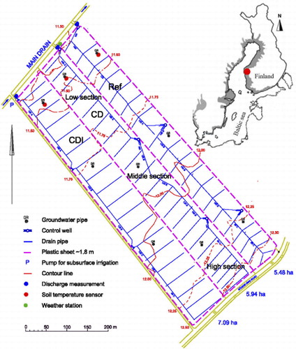
The study site is located in the Söderfjärden meteorite crater (2300 ha) with holocene sulfide-bearing marine sediments at an altitude of c. 2 m above the current sea level, 6 km from the coast line, 10 km south of the town of Vasa in western Finland (Figure 1). In order to form arable land, a large drain ditch was dug and a pumping station built in 1926. The area was pipe drained first in the 1950s. The subsurface drains for the whole area were renewed in the 1990s, equipped with control wells to enable regulation of the drainage. By aid of reclamation and extensive surface liming, the area has become part of the most productive and expensive farmlands in Finland. Extensive studies have been conducted on the land in the area (Nordmyr et al. 2006). The sulfides in the parent sediment materials contain nearly equal amounts of reactive monosulfides (FeS_n; n = 1.0–1.3) and pyrite (FeS₂), while the upper horizons (down to c. 1.5–2.0 m below surface) have been oxidized and developed into structured AS soils that are typical of the region (Boman et al. 2008).

Figure 1. Location of the Söderfjärden experimental field (red dot in the map) and layout of the drainage/monitoring system in the experimental field. The contour line indicates the elevation above the mean sea level +10 m (to avoid negative values) according to the Finnish N60 system (mean sea level in 1960). Due to the rapid land uplift (c. 8 mm a⁻¹), the land is c. 40 cm higher above the mean sea level today, e.g., 11.5 m in the N60 + 10 m system on the map equals 1.9 m above the current mean sea level.

Experimental field

Three adjacent fields (total area: 18.4 ha), each c. 80–100 m wide and c. 710–740 m long, with previously installed subsurface drainage pipes with control wells were selected as experimental site (Figure 1). The surface of the lower part, closest to main drain, is c. 1.9 above mean sea level (MSL) and the area furthest from the main drain is c. 2.9 m above MSL. Thus, to enhance the possibility to regulate the groundwater for the whole field, each field has three control wells that drain/divide the field into three sections, below referred to as “low,” “middle,” and “high section” (Figure 1). The water from the well of the high section runs through that of the middle and low section before discharged into the main open drain northwest of the fields. The lateral and collector pipes had been installed at c. 1.2 m and 1.3–1.5 m depth, respectively.

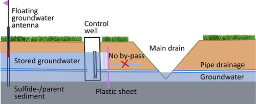
In order to prevent by-pass flow, all three test fields were in June 2010 hydrologically isolated from each other and from the main drain with vertical plastic sheets from 0.3 m depth down to the impermeable massive parent sediment at 1.8 m depth (Figure 2). Thus, water from the fields can positively only be removed by drainage through the subsurface drain pipes or by evapotranspiration. The installation and use of plastic sheets to prevent by-pass flow in CD systems is a new technique described in Österholm and Rosendahl (2012).

Figure 2. On the left: controlled pipe drainage used to store excess groundwater, a plastic sheet to prevent by-pass flow and a floating groundwater antenna for manual/visual groundwater monitoring. On the right: conventional pipe drainage (similar to Ref but without plastic sheet) causing a rapid groundwater drop (Reproduced from Österholm and Rosendahl 2012).

In CD and CDI (Figure 1), the outflow in the control weirs was set to 0.7 m below the lowest point of each field during the winter season and to 0.6 m during the summer season from the end of May until September/October (Figure 2). In CDI, subsurface irrigation was conducted by pumping water from the main drain into the control well of the low section in order to artificially raise the groundwater level in the whole field. In a reference field (Ref in Figure 1), there was no regulation, equaling drainage conditions with conventional pipe drainage with the exception that Ref was isolated from the main drain by the plastic sheet.

Perforated groundwater pipes were installed in each fields low section to the depth of 2.5 m; one for a groundwater logger (EHP-QMS) in each fields low section and separate groundwater pipes in all field sections for manual groundwater measurements with a “floating antenna” (Figure 2). The floating antenna is a cheap and easy method that was developed to enable farmers to monitor and properly manage the groundwater level. The antenna is made of plastic pipe (diameter: 20 mm) with a foam floater in the bottom (sinks 30 cm below groundwater surface), rising and falling with groundwater fluctuations. Consequently, the groundwater depth (GW, cm) can be calculated from the total length of antenna (A_lenght, cm), the elevation of the top of antenna above soil surface (A_top, cm) and the sinking depth of floater (30 cm) according to:

Precipitation was obtained from the national Skatila weather station maintained by the Finnish Environment Institute and located c. 30 km NE of our experimental site. Due to the very flat topography and similar distance to the sea, the overall annual precipitation, mainly caused by low-pressure fronts, is similar between the locations. However, the occurrence and intensity of occasional rain events may differ significantly between the sites.

In order to monitor the water flow in drainage outlets, an EHP-Ultrasonic Flow monitoring system was installed at the control wells in the lower part of each experimental field. The system is a combination of an EHP DL-6 data logger with a gsm/gprs-modem, Fluxus 5107 ultrasonic device, 2 m long EHP-pipe, accumulators, and solar panels. Ultrasonic sensors were installed outside the EHP-pipe to measure flow velocity (m s⁻¹). The discharge (L s⁻¹) was calculated on the basis of the flow velocity and the diameter of the EHP pipe.

Soil sampling and analysis

Soil profiles were sampled in the autumns of 2009 and 2011–2013 with an auger at vertical depth intervals of 20 cm from the surface down to a depth of 2 m in the middle of each subfield. The pH (1:1) in deionized water was measured in the field (e.g., Österholm & Åström 2002). Results of duplicate measurements were within ±0.2 pH units.

In the autumn of 2013, titratable actual acidity was determined on the fresh soil samples, taken at depths between 40 and 200 cm from the middle of each subfield, according to Ahern et al. (2004). Deviations between routine and 10 duplicate samples were <13%.

Water soluble salts were analyzed from the fresh soil samples, taken at depths between 0 and 0.60 cm from the middle of each field in 2013. The samples were extracted with deionized water at a ratio of 1:60 (w/v). Soils were agitated in an end-over end shaker for 1 hour and filtrated through a 0.2-µm membrane filter (Whatman, Maidstone, UK). Concentrations of S, Ca, Mg, P, K, and Na were analyzed with ICP-OES (Perkin Elmer Optima 8300) and concentration of Cl with skalar (Skalar San⁺⁺ System). Electrical conductivity (EC) was measured from samples mixed with deionized water at a ratio 1:2.5, w/v. All samples were analyzed in duplicate.

Pedological features were recorded in a 220-cm deep soil pit dug c. 300 m N of the actual experimental field in soil which in terms of texture, elevation, and water regime was similar to the experimental field (without hydrologic isolation). The soil was analyzed by the horizon for total C and S by dry combustion using a LECO apparatus (e.g., Österholm & Åström 2002). Particle size distribution was determined with the pipette method after removal of organic matter with H₂O₂ and HCl and dispersion of the sample with Na₄P₂O₇ (Elonen 1971).

Results

General soil properties and pedological features

The investigated soil profile had a 28-cm deep ploughed ochric epipedon (Soil Survey Staff 2014). This Ap horizon had a silt loam texture while all subsoil horizons were silty clay loam. The cambic Bgj1 horizon (28–50 cm) had a fine-to-medium angular blocky structure with a gleyic color pattern. The aggregates had brown iron hydroxide and yellow jarosite coatings while the interiors were gray. The thickest coatings occurred in the Bgj2 horizon (50–86 cm) which had a weak medium prismatic structure, parting to strong angular blocky aggregates. Oxidation was visible down to the bottom of the Bg horizon (86–152 cm), which, however, had much weaker coatings on the aggregate surfaces than the horizons above. This horizon consisted of very coarse (length: 30–40 cm) prismatic aggregates. There were permanent shrinking cracks between the prisms, conducive to substantial by-pass flow of water. Minor roots were found down to c. 150 cm. The Cg horizon below 150 cm had a massive structure. A few initial desiccation cracks extended down to 180 cm but they had no iron hydroxide coatings, indicating that the horizon is permanently in the reduced state. While the total sulfur in the B horizons was 0.2–0.4%, it increased to 0.8% in the Cg horizon containing reactive black monosulfidic materials. The concentration of organic carbon was relatively high, in the order of 2% throughout the soil profile with no distinctive accumulation in the top soil. The hydraulic conductivity of the reduced unstructured subsoil was remarkably low; only minor amounts of groundwater could be observed at the bottom of the 220-cm deep soil pit after 6 hours although the water level in the main drain 20 m away was up to 1 m higher. According to Soil Taxonomy (Soil Survey Staff 2014), the soil belongs to Sulfic Cryaquepts and to Thionic Gleysols (drainic, humic, loamic/siltic) according to the WRB system (IUSS Working Group WRB 2014).

Soil pH and acidity

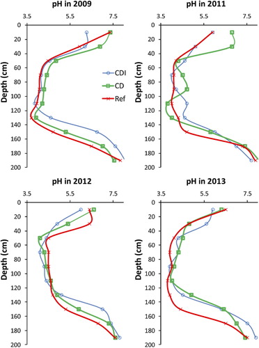
The vertical distribution of pH is relatively similar in the different treatments (Figure 3). The pH values were lowest at depths between 60 and 140 cm, typically slightly above 4 in all profiles and occasionally just below pH 4 (Figure 3). However, pH in the plough layer (0–20 cm) of CDI was significantly lower (average pH in 2011 to 2013 = 5.9) than in CD (pH 6.6) and Ref (pH 6.3). Moreover, as compared to Ref the depth of oxidation, as indicated by pH, seems to be c. 20 cm shallower in the CDI field.

Figure 3. pH in profiles from the low-field sections in the autumns of 2009 (prior to field experiments) and 2011–2013.

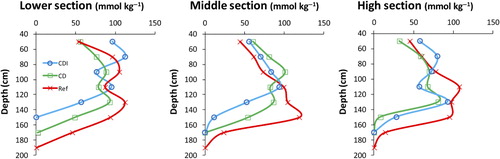
As expected for AS soils, the actual acidity was extremely high above 1.5 depth in all field sections, generally being between 50 and 100 mol kg⁻¹ down to 160 and 180 cm in the Ref, 140–160 cm in CD and 140 cm in CDI (Figure 4). The acidity was relatively low, close to 50 mmol kg⁻¹ in the 40–60 depth with the exception of the lower CDI field where it was twice as high.

Figure 4. Actual acidity (mmol kg⁻¹) in the low, middle, and high sections in November 2013.

Water balance

The annual precipitation varied significantly during the study period, 562–748 mm, within a range typical for the area (Table 1). Variations in the annual discharge were, however, remarkably small; in Ref 244–278 mm, comprising less than half (37–46%) of the annual precipitation in each of the 3 years, the latter highlighting the role of evapotranspiration in this Boreal farmland. As compared to Ref, the annual discharge in CD varied somewhat more (280–336 mm) and was 21–58 mm higher. Consequently, the calculated evapotranspiration was smaller. The discharge, thus, equals c. 44–50% of precipitation and the evapotranspiration c. 50–56% of precipitation. In 2012, the discharge in CDI was 33 mm higher than in Ref, almost corresponding to the high amount of sub-irrigation (50 mm). In 2011, however, there was no significant difference (5 mm) between the treatments and in 2013, with only 12 mm of sub-irrigation, the discharge was 24 mm lower in CDI. Evapotranspiration was the highest in CDI in all years; the discharge and evapotranspiration were 36–41% and 59–64% of precipitation plus sub-irrigation, respectively.

Table 1. The water balance of the different treatments assuming zero surface runoff.

	CDI			CD			Reference
	2011	2012	2013	2011	2012	2013	2011	2012	2013
Precipitation (mm a^−^1)	658	748	562	658	748	562	658	748	562
Sub-irrigation/pumping (mm a^−^1)	31	50	12	–	–	–	–	–	–
Drainage/discharge (mm a^−^1)	249	311	235	292	336	280	244	278	259
Evaporation (mm a^−^1)	439	487	339	366	412	282	414	470	303

Groundwater table

The manual groundwater measurements with “floating antennas” produced results that were mostly within ±10 cm of those of the data loggers (Figure 5). The most notable deviation occurred in the late summer of 2013, when three consecutive manual groundwater measurements overestimated the data logger groundwater depth with 20–40 cm in CD (Figure 5).

Figure 5. Air temperature, 5-day precipitation in Skatila and the depth of groundwater measured with a logger (continuous line) and manually (filled circles). In the lowermost graph, the critical sulfidic horizon is shaded, the average depth of lateral subsurface drains is indicated with a horizontal line and sub-irrigation events in the CDI field are indicated with arrows.

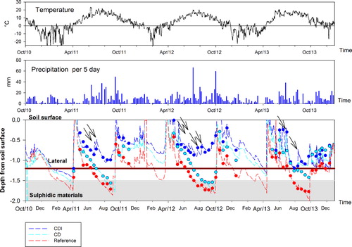
The general large-scale temporal fluctuations in groundwater table within each year were largely dependent not only on rain and evapotranspiration but also on cold conditions in winters resulting in snow and frost. During the study period, rainfall excess during late autumns raised the groundwater until sub-zero temperatures prevailed (November to December; Figure 5), and, consequently, precipitation occurred mainly as snow. As indicated by the soil temperature sensor at 30 cm depth (data not shown), significant frost developed in January. Under such conditions, the groundwater moved downwards slowly but rather continuously, being very deep (c. 150 cm) in late winters. However, in 2012, the groundwater was relatively high and stable in January to February, coinciding with a notably high sea water level preventing the transport of drainage water to the sea, above zero temperatures and significant precipitation in January (Figure 5). The thaw melted each year in March to April, soon after the average air temperatures increased above zero. Coinciding with these events, the groundwater level rose very rapidly close to soil surface within 1–2 weeks in all years due to meltwater percolation.

Reference field

In Ref, the groundwater fluctuated between 0 and 2 m (Figure 5). The groundwater level in the low section was below the drainage depth most of the year (232–281 d a⁻¹) and below the critical sulfidic depth (150 cm) for 83–105 d a⁻¹ (Table 2). In the middle and high sections, a similar trend was observed but there the groundwater table dropped even deeper. In the high section, the deepest measured depth was 2.2 m below surface. The groundwater dropped down to the maximum subsurface drainage depth (c. 1.4 m, laterals c. 1.2 m) in late June in 2011–2012 and early July in 2013 and it continued to drop continuously, being below the critical sulfide depth during 9 July–2 September in 2011, 10 July–1 October in 2012, and 23 July–27 September in 2013. The lowest level of the groundwater table 1.8 m in 2011–2012 and 2.0 m in 2013 was all years reached in September. It is notable that after the groundwater level had dropped to a level below c. 1.2 m in early summers, rain events with up to 70 mm in 5 days in July 2012, had no more effect on the groundwater level. On the contrary, in late September 2011 and 2012, after harvesting and temperatures near 10°C, 50–60 mm of rain in 5 days was enough to rapidly raise the groundwater from the critical sulfidic horizon to near surface.

Table 2. The number of days when the groundwater level was below the drainage depth or below the critical sulfide depth at 1.5 m.

		CDI			CD			Reference
		2011	2012	2013	2011	2012	2013	2011	2012	2013
Below sub-drain pipes	Day/year	91	0	88	175	94	133	232	241	281
In critical sulfide depth	Day/year	0	0	0	53	45	0	105	83	91

Controlled drainage

Temporal variations in the level of groundwater table in CD were similar to those of Ref (Figure 5). The rapid increase in groundwater level to near surface in late autumns and during snow melt in spring followed by a drop, coincided with that of Ref. In the end of May, before the control level was raised from 70 cm, set for the winter seasons, to 60 cm for the summer seasons, the groundwater was already 20–30 cm below the winter control level in all years. The groundwater was, however, 10–20 cm higher than in the Ref. During summer, the groundwater drop was delayed and it was generally 10–20 cm higher and occasionally >40 cm higher than in Ref (e.g., the summer of 2013). Although the groundwater dropped to 1.7–1.8 m in the summers of 2011–2012, similar to that in Ref, the groundwater was below the critical sulfide depth (150 cm) for a significantly shorter time than in Ref, i.e., extending for 0–53 d a⁻¹ (Table 2). In 2013, in contrast to previous years, there was a remarkable difference between the treatments. While the groundwater in the low section of Ref stayed below the critical sulfide depth for 91 days, it stayed around the depth of c. 1.1 m in CD and was never below the critical depth (Table 2). However, in the middle and high sections, it dropped below the critical sulfide depth in late August. In the following autumn, with low precipitation, the groundwater stayed around 1 m and did not approach the control depth until January. Unlike Ref, in winters, there seems to be a minor risk of a significant groundwater drop into the critical sulfidic horizon although it was shown in March 2011 that it may be possible for a brief time (Figure 5).

Controlled drainage with subsurface irrigation

In CDI, the temporal variations in the groundwater table were similar to those of Ref and particularly with CD (Figure 5). The rapid rises of groundwater to near surface in late autumns and during snow melt in spring coincided with the ground water rise in the two other treatments. In the end of May 2011–2012, before the control level was raised up to 50 cm below surface for the summer season, the groundwater was near the winter control level (c. 60 cm) and that was 30–40 cm higher than in Ref. In 2013, the groundwater had, however, already dropped c. 30 cm below the winter control level being close to the groundwater level in Ref.

Similar to CD, the drop in groundwater level was slower in CDI, than in Ref, but in contrast to both other treatments, the groundwater level was raised by c. 10–20 cm during 2–4 sub-irrigation events in summers (Figure 5). The differences in lowest groundwater depths during summers, as compared to CD, corresponded to the amount of sub-irrigation; the lowest groundwater depth was only c. 70 cm in the summer 2012 (c. 170 cm in CD), c. 100 cm in 2011 (c. 170 cm in CD), and c. 120 cm in 2013 (similar to CD). It is notable that in the winters of 2011 and 2013, the groundwater dropped to 1.2–1.3 m, being just slightly higher than in CD. Most importantly, in all sections of CDI and during the whole study period, the groundwater never dropped below the critical sulfidic horizon, and it was above the drain pipe depth most part of each year (Table 2).

Soluble salts

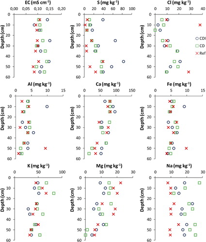
Considering vertical trends in all fields, soluble Cl and S increased while Ca and Mg decreased with depth (Figure 6). No vertical trends were found for Al, Fe, K, or Na. The EC was relatively stable, being between 0.09 and 0.11 mS cm⁻¹ for all depths in Ref. As compared to Ref, EC was slightly higher (0.11–0.12 mS cm⁻¹), Na about twice as high (medians 10, 22, and 17 mg kg⁻¹ in Ref, CD and CDI, respectively), and S strongly higher in CD and CDI (medians 6, 24, and 39 mg kg⁻¹ in Ref, CD and CDI, respectively). The highest EC (0.14–0.15 mS cm⁻¹), corresponding to the highest concentrations of S (39–83 mg kg⁻¹), was found in the profile closest to the drain in CDI. Apart from S, there were no significant spatial trends with the distance to the main drain.

Figure 6. Water soluble salts in the CDI, CD, and Ref. To enable distinction of field sections, the low sections are plotted 5 cm lower and the high sections 5 cm higher than their actual depth below surface.

Discussion

In the present study, by-pass flow into the main drain or to adjacent fields was expected to be prevented by vertical plastic sheets extending down to a depth of c. 1.8 m. The importance of the hydrological isolation with the plastic sheet was proven particularly in CDI where the gradient between the groundwater level in the field and in the main drain was the greatest, and particularly since the groundwater remained high for a long time regardless the strongly structured B horizons. In CDI, the groundwater never dropped to the critical sulfide depth in the course of the experimental period (Table 2) even if during mean sea water levels, the maximum theoretical drainage depth, i.e., height difference between drains and MSL, was c. 2 m or more. Further evidence for the importance of plastic sheet was provided by experience from a subsurface irrigation trial prior to the installation of plastic sheets; the farmer and the drainage technician observed significant by-pass flow through the wall of the main drain and the groundwater dropped much faster. However, even after installation of plastic sheets, the groundwater in CD dropped near the critical sulfide depth during winters when the sea water was relatively low (deviation from MSL typically less than ±0.5 m in the Baltic Sea), indicating that some leakage might occur from the latter field.

Assuming that no leakage to the open drain occurred, groundwater could theoretically drop down to a depth of 1.4 m in the low section of Ref due to subsurface drainage, and due to the control levels down to c. 0.6–0.7 m in CD and CDI. However, in the lower section of CD, groundwater dropped from the winter control level (0.7 m) to c. 1 m in late May and further down to c. 1.7–1.8 m in early autumn, indicating that evapotranspiration played a major role in lowering the groundwater level in summers. The faster groundwater drop in Ref, exposed the subsoil horizons to atmospheric oxygen for a relatively long time. Even though the maximum groundwater depth was only c. 20 cm lower in Ref than in CD, the maximum depth in CD was reached a couple of weeks later than in Ref. In CDI, however, the groundwater drop was not only strongly delayed but up to 1 m higher than in Ref, and it was also clearly above the critical sulfide depth all along the study period. Thus, our results indicate that a higher groundwater level and prevention of oxidation of sulfidic materials in subsoil will be obtained by using the CDI method. With CD, it may be difficult to prevent the groundwater from dropping down to the sulfidic subsoil in previously conventionally drained soils. The main positive effect with CD seems to be that the time of exposure to oxygen is reduced, which is also well in line with that of Åström et al. (2007). In contrast to studies on farmlands with CD in Sweden (Wesström et al. 2001; 2003) and in North Carolina (Gilliam et al. 1997), the discharge was not decreased and due to input of excess water evapotranspiration was only slightly higher in CDI.

The observed groundwater levels (≥1.5 m) in Ref and CD corresponded well to the pedogenic features of soil development, i.e., the strong structure development combined with a low pH and high acidity down to this depth. Consequently, this is that part of the profile which currently releases acidity and metals into water courses, at such a rapid rate that the pool of sulfur/acidity is halved within a few decades (Österholm & Åström 2004). The reduced massive parent sediment having a low hydraulic conductivity contains a large pool of sulfides (c. 0.8%) that has not yet released acidity but obviously will do so in case the groundwater drops further and allows soil structure to develop. Although not significant, the soil pH differences along the experiment period indicate that in Ref the pH may have been lowered (Figure 3). No obvious change could be observed in the pH temporal patterns in CD or CDI. The actual acidity in Ref sections was 14–46 mmol kg⁻¹ at the depth of 1.7 m, whereas it was still zero in CD and CDI after the treatments. It is notable that the soil above the reduced subsoil horizons was not yet completely oxidized, which was indicated by the fact that they still contained significant amounts of sulfides, mainly as pyrites reported in a previous study (Boman et al. 2008). Interiors of soil aggregates may have remained relatively wet during summer preventing complete oxidation. Consequently, a higher groundwater may also decrease the production of further acidity from the semi-oxidized soil horizons (above 1.5 m). Moreover, in the presence of easily decomposable organic matter, reduction of sulfates and ferric iron may re-form iron sulfides and, thus, buffer the soil acidity, if a reducing environment can be created (Rabenhorst et al. 2006; Burton et al. 2011). In the present study, there were no indications of sulfide formation or reduced acidity in CDI or CD during the time of study (3 years). Since there may be a lack of easily decomposable organic matter and since boreal AS soils are rich in reactive iron oxides (Österholm Åström 2002; Virtanen, Simojoki, Hartikainen et al. 2014) and the soil temperature regime is cryic, it is possible that sulfides cannot be re-formed or that the process is very slow in this environment. Nevertheless, in a lysimeter experiment, Virtanen, Simojoki, Rita et al. (2014) found that in cultivated lysimeters, where decomposable organic matter was available for microbes, the soil pH rose in the 2.5-year experiment due to reduction reactions and lowered Al concentrations in the soil solution and discharge. In the present study, only minor roots extended to depths below 1 m, and, thus, input of fresh organic matter is probably very limited to the inundated soil horizons.

When water evaporates, the dissolved salts are left behind to accumulate in the soils if there is insufficient rainfall and drainage to leach them to lower soil horizons, groundwater, or drain pipes. In boreal conditions, the yearly precipitation exceeds evapotranspiration and therefore accumulation of salt is not common. However, in boreal AS soils, accumulation of metal-sulfate salts (including Al) was a typical feature in the past (Kivinen 1944) but by drainage, contribution from capillary rise as well as salt accumulation in the soil surface was cut down. Thus, an important aim of water management at that time, when sulfidic sediments were commonly reclaimed for agriculture and environmental concern was of less importance, included creating conditions that leached the acidity and toxic Al from the soil. Making the drainage more efficient with subsurface drain pipes also decreases the need for surface liming (Palko 1994). Therefore, we were concerned that rising groundwater may increase the capillary rise of water rich in dissolved salts to replace the water lost in the upper horizons by evapotranspiration as reported by Minh et al. (1998).

According to our findings, soluble S and Cl increased with depth, which in the case of S was expected since the subsoil contains very high concentrations of S (Figure 6). However, in CD and, in even more so CDI where the average groundwater was highest, the highest concentrations of S compared to Ref were observed. It is less likely that this higher salt content in CDI was directly caused by S and Cl from the irrigation water, since the other studied elements, also present in the irrigation water, did not show the same trend. Consequently, accumulation can be explained by capillary rise of inherent sulfates from the subsoil. Nevertheless, in terms of EC (Figure 6), the total amount of salts was not alarming, indicating that any potential accumulation of salts during summer is flushed away during high flow. Thus, CD and CDI did not cause marked accumulation of monovalent ions that could promote degradation of soil structure. Neither did CD and CDI enhance accumulation of Al as had been observed in the middle of the twentieth century. However, the significantly lower pH and S in the uppermost 20 cm in CDI may be related to an increased capillary rise of subsoil acidity that increases the need for surface liming.

While it is uncertain if the oxidation process in the Boreal AS soils can be reversed into acid consuming sulfate reduction by raising the groundwater, management that prevents oxidation of sulfides, i.e., formation of new acidity, in the lower subsoil will improve the water quality in future. More extreme weather conditions, i.e., intensive droughts followed by floods, due to potential climate change, pose an obvious risk for increased oxidation (Österholm & Åström 2008; Simek et al. 2011). The CD and CDI systems are rather easy to operate and they have the potential to decrease the oxidation but this requires proper management by the farmers. Proper management requires knowledge of the groundwater fluctuations in the field. The floating antenna proved to be an easy and reliable tool for monitoring the groundwater and can therefore be strongly recommended to be used in association with groundwater management in controlled drainage systems.

Acknowledgments

Vincent Westberg and his colleagues at the Vasa ELY-center have provided invaluable help during the project. We also want to acknowledge pioneer farmers Stefan Östman, Arne Lervik, Tom Backlund, and Mats Nylund as well as the excavation company Backlunds Gräv for their cooperation and innovativeness.

Disclosure statement

No potential conflict of interest was reported by the authors.

Additional information

Funding

This study has been conducted within the framework of the EU-Life + program in a project titled Climate Change Adaptation Tools for Environmental Risk Mitigation of Acid Sulfate Soils (CATERMASS) and later within a program financed by the Finnish Ministry of Agriculture and Forestry. Additional financial support has been provided by Finnish Drainage Foundation Finnish Field Drainage Association, Maa- ja vesitekniikan tuki ry and Renlunds foundation.

References

- Ahern CR, McElnea AE, Sullivan LA. 2004. Acid sulfate soils laboratory methods guidelines. Queensland: Queensland Department of Natural Resources, Mines and Energy, Indooroopilly, 186 p.
- Åström M, Österholm P, Bärlund I, Tattari S. 2007. Hydrochemical effects of surface liming, controlled drainage and lime filter drainage on boreal acid sulfate soils. Water Air Soil Pollut. 179:107–116.
- Bärlund I, Tattari S, Yli-Halla M, Åström M. 2004. Effects of sophisticated drainage techniques on groundwater level and drainage water quality on acid sulphate soils – Final report of the HAPSU project. The Finnish Environment 732. 68 p. Available from: http://www.environment.fi/publications
- Boman A, Åström M, Fröjdö S. 2008. Sulfur dynamics in boreal acid sulfate soils rich in metastable iron sulfide: the role of artificial drainage. Chem Geol. 255:68–77. 10.1016/j.chemgeo.2008.06.006
- Burton ED, Bush RT, Johnston SG, Sullivan LA, Keene AF. 2011. Sulfur biogeochemical cycling and novel Fe-S mineralization pathways in a tidally re-flooded wetland. Geochim Cosmochim Acta. 75:34–51.
- Dent D. 1986. Acid sulphate soils: a baseline for research and development. Wageningen: ILRI-publication 39; p. 204.
- Elonen P. 1971. Particle-size analysis of soil. Acta Agralia Fennica 122:1–122.
- Gilliam JW, Osmond DL, Evans RO. 1997. Selected agricultural best management practices to control nitrogen in the Neuse River basin. North Carolina Agricultural Research Service Technical Bulletin 311. Raleigh, NC: North Carolina State University Press; p. 53.
- Hudd R. 2000. Springtime episodic acidification as a regulatory factor of estuary spawning fish recruitment. [Academic dissertation]. Helsinki: Department of Limnology and Environmental Protection University of Helsinki, Finnish Game and Fisheries Research Institute.
- IUSS Working Group WRB. 2014. World reference base for soil resources 2014 – International soil classification system for naming soils and creating legends for soil maps. Rome: World Soil Resources Report No. 106. FAO.
- Joukainen S, Yli-Halla M. 2003. Environmental impacts and acid loads from deep sulfidic layers of two well-drained acid sulfate soils in western Finland. Agric Ecosyst Environ. 95:297–309. 10.1016/S0167-8809(02)00094-4
- Kivinen E. 1944. Aluna- eli sulfaattimaista. J Sci Agric Soc Finland. 16:147–161. Finnish.
- Minh LQ, Tuong TP, van Mensvoort MEF, Bouma J. 1998. Soil and water table management effects on aluminum dynamics in an acid sulphate soil in Vietnam. Agric Ecosyst Environ. 68:255–262. 10.1016/S0167-8809(97)00158-8
- Nordmyr L, Boman A, Åström M, Österholm P. 2006. Estimation of leakage of chemical elements from boreal acid sulphate soils. Boreal Env Res. 11:261–273.
- Österholm P, Åström M. 2002. Spatial trends and losses of major and trace elements in agricultural acid sulphate soils distributed in the artificially drained Rintala area, W. Finland. Appl Geochem. 17:1209–1218.
- Österholm P, Åström M. 2004. Quantification of current and future leaching of sulfur and metals from Boreal acid sulfate soils, western Finland. Aust J Soil Res. 42:547–551.
- Österholm P, Åström M. 2008. Meteorological impacts on the water quality in the Pajuluoma acid sulphate soil area, W. Finland. Appl Geochem. 23:1594–1606.
- Österholm P, Rosendahl R. 2012. By-pass flow prevention on farmlands with controlled drainage. In: Österholm P, Yli-Halla M, Edén P, editors. Proceedings of the 7th International Acid Sulfate Soil Conference, Vaasa: Geological Survey of Finland, Guide 56; p. 169–171.
- Palko J. 1994. Acid sulphate soils and their agricultural and environmental problems in Finland [Academic dissertation]. Oulu: Acta Universitatis Ouluensis. C 75, University of Oulu.
- Rabenhorst MC, Fanning DS, Burch SN. 2006. Acid sulfate soils: formation. In: Lal R, editor. Encyclopedia of soil science. 2nd ed., Volume 1. New York, NY: Taylor & Francis Group, LLC; p. 20–24.
- Rickard D, Luther GW. 2007. Chemistry of iron sulfides. Chem Rev. 107:514–562. 10.1021/cr0503658
- Simek M, Virtanen S, Kristufek V, Simojoki A, Yli-Halla M. 2011. Evidence of rich microbial communities in the subsoil of a boreal acid sulphate soil conducive to greenhouse gas emissions. Agric Ecosyst Environ. 140:113–122. 10.1016/j.agee.2010.11.018
- Sohlenius G, Öborn I. 2004. Geochemistry and partitioning of trace metals in acid sulphate soils in Sweden and Finland before and after sulphide oxidation. Geoderma. 122:167–175. 10.1016/j.geoderma.2004.01.006
- Soil Survey Staff. 2014. Keys to soil taxonomy. 12th ed. Washington, DC: USDA-Natural Resources Conservation Service.
- Sundström R, Åström M, Österholm P. 2002. Comparison of the metal content in acid sulfate soil runoff and industrial effluents in Finland. Environ Sci Technol. 36:4269–4272.
- Virtanen S, Simojoki A, Hartikainen H, Yli-Halla M. 2014. Response of pore water Al, Fe and S concentrations to waterlogging in a boreal acid sulphate soil. Sci Total Environ. 466–467:663–667.
- Virtanen S, Simojoki A, Rita H, Toivonen J, Hartikainen H, Yli-Halla M. 2014. A multi-scale comparison of dissolved Al, Fe and S in a boreal acid sulphate soil. Sci Total Environ. 499:336–348. 10.1016/j.scitotenv.2014.08.088
- Wesström I, Ekbohm G, Linnér H, Messing I. 2003. The effects of controlled drainage on subsurface outflow from level agricultural fields. Hydrol Process. 17:1525–1538.
- Wesström I, Messing I, Linnér H, Lindström J. 2001. Controlled drainage – effects on drain outflow and water quality. Agric Water Manage. 47:85–100.
- Wu X, Wong ZL, Sten P, Engblom S, Österholm P, Dopson M. 2013. Microbial community potentially responsible for acid and metal release from an Ostrobothnian acid sulfate soil. FEMS Microbiol Ecol. 84:555–563. 10.1111/1574-6941.12084