A simplified method for determination of Philip-Dunne infiltration parameters

ABSTRACT

The Philip-Dunne falling-head infiltration for determining the parameters of soil water movement is a relatively simple procedure, yet the calculation is still complicated. This study develops a simplified method for determining soil saturated hydraulic conductivity k_s and Green-Ampt wetting front suction ψ. Field Philip-Dunne infiltration tests are performed in a loam soil under different initial head heights (30, 40, and 50 cm) at 45 test points. The relationship between infiltration time t_i and the parameters k_s and ψ is explored. The results show that Δθ within the range of 0.015–0.147 has little influence on k_s or ψ in the test soil, and prediction of the two parameters using mean Δθ meets the accuracy requirements. k_s is significantly negatively correlated with t_i and best predicted by 1/t_med; the prediction accuracy of the linear function is strongly influenced by the initial head height h₀. There is a significant relationship between ψ and t_max/t_med, and h₀ has little influence on the prediction accuracy of the power function. Therefore, the simplified models based on 1/t_med and t_max/t_med can be used for field-scale determination of the parameters k_s and ψ in loam soil, with an overall error below 10%.

KEYWORDS:

• Philip-Dunne method
• saturated hydraulic conductivity
• wetting front suction
• prediction model
• vertical infiltration

Introduction

Infiltration is the process by which water on the ground surface enters the soil. It is an important part of the conversion between atmospheric precipitation, surface runoff, soil water, and groundwater (Derby et al. 2013; Zhang et al. 2015). Research into this process is of practical significance for increasing soil infiltration and preventing soil erosion, which in turn contributes to ecological construction and agricultural production (Angelaki et al. 2013). Therefore, a large body of work has been conducted on the application of infiltration models, determination of infiltration parameters, and error analysis (Yang et al. 2015; Liang et al. 2020; Lu et al. 2019).

Soil saturated hydraulic conductivity k_s and Green-Ampt wetting front suction ψ are two important parameters of soil water movement strongly influence by multi-factors, such as soil texture, soil structure, and land-use pattern (Mao et al. 2016; Hsu et al. 2017; Réfloch et al. 2017; Tsai et al. 2018). Both the parameters k_s and ψ can be determined using constant-head or falling-head methods through various infiltration models (Sadeghi et al. 2012; Reynolds 2013; Ma et al. 2015; Leung et al. 2018; Zhao et al. 2019). Generally, falling-head infiltration is more popular than constant-head infiltration for the determination of soil water parameters, because constant-head methods using a single-ring infiltrometer, double-ring infiltrometer, or Guelph permeameter require a stable state to be achieved. It would cost a long time to reach a stable infiltration rate in soils with a low hydraulic conductivity, while a large amount of water is required in soils with high hydraulic conductivity (Chen and Hsu 2012; Malama and Revil 2014; Mohammadzadeh-Habili et al. 2018).

The Philip-Dunne method is a falling-head infiltration model proposed by John Philip in 1993, based on the soil water data from the Amazon basin and the basic assumption of the Green-Ampt model (Philip 1993). Since its emergence, the Philip-Dunne method has received increasing attention of many researchers. De Haro et al. (1998) evaluated the practical applicability and application conditions of the Philip-Dunne method through a sensitivity analysis of the parameter k_s. Gómez et al. (2001) compared the infiltration models of infiltration ring, tension permeameter, and precipitation simulator versus Philip-Dunne infiltration, and they found that the k_s values determined by different methods were close to each other, yet the ψ values were substantially different.

Muñoz—Carpena et al. (2002) obtained relatively large k_s and ψ values from the Philip-Dunne infiltration compared with the constant-head well infiltration and attributed this discrepancy to differences in soil volume, soil anisotropy, and infiltration shape. To promote the application of the Philip-Dunne method, Garcıa-Sinovas et al. (2002) designed an innovative instrument that could automatically read the water level-time course, namely the Philip-Dunne permeameter (Muñoz-Carpena et al. 2002). Although the Philip-Dunne permeameter for determining the parameters of soil water movement requires a relatively simple procedure, the calculations are still complicated.

To simplify the calculation of the parameters k_s and ψ, this study performs field infiltration tests using the Philip-Dunne method in a loam soil. The relationships between infiltration time t_i, soil water content change Δθ, and the parameters k_s and ψ are analyzed. Simplified models are constructed for predicting k_s and ψ based on t_i. This study provides a practical tool for field-scale determination of the parameters k_s and ψ at sites with a single homogeneous soil texture.

Materials and methods

Test soil

The test site was located in Ludong University (Yantai, Shandong Province, China) and was part of a bare field where wheat had been harvested. Soil samples were taken from a depth of 0–30 cm at three random points. The soil samples were air-dried and passed through a 2-mm sieve. Particle size distribution was determined using a Mastersizer 2000 particle size analyzer (Malvern Instrument Inc., Worcestershire, UK), which showed that the soil contained 11.9% clay, 49.3% silt, 36% fine sand, and 2.8% coarse sand. Soil texture was classified as a loam soil according to Soil Survey Staff (1960).

Infiltration test and data collection

From April to May 2019, field tests were carried out at 45 test points (37.5 points 1000 m⁻²) for each head height uniformly arranged in a 40 m × 30 m plot. To analyze infiltration in the initially unsaturated soil, falling-head infiltration test was performed at each point using the Philip-Dunne method (Muñoz-Carpena et al. 2002). The infiltration instrument mainly consisted of a Philip-Dunne permeameter which contained a transparent plastic tube (inner radius r_i= 4.2 cm), and the initial head height was set to 30, 40, and 50 cm separately. Before the test, three 10-cm deep boreholes were drilled in the soil at each point. Then the transparent plastic tube was vertically placed in each borehole, with no gap between the tube wall and borehole sidewall. The bottom of each tube was wrapped using a plastic film. Then, water was injected into the parallel tubes to reach different head heights (h₀ = 30, 40, and 50 cm, respectively). Afterwards, the plastic film was removed to start the infiltration test (t = 0).

During the infiltration process, the time required for every 5 cm of decrease in water level inside the tubes was recorded. Specifically, t₅, t₁₀, t₁₅, t₂₀, and t₃₀ were recorded at h₀ = 30 cm; t₅, t₁₀, t₁₅, t₂₀, t₂₅, t₃₀, and t₄₀ were recorded at h₀ = 40 cm; and t₅, t₁₀, t₁₅, t₂₀, t₂₅, t₃₀, t₃₅, t₄₀, and t₅₀ were recorded at h₀ = 50 cm. In addition, the time to reach half of the initial head height h₀/2 (medium infiltration time, t_med) and the time to finish infiltration (maximum infiltration time, t_max) were recorded. The initial volumetric water content (%) before infiltration θ₀ and the final water content after infiltration θ_s in the 0–10 cm surface soil were measured using a Trime-T3 tubular TDR system (IMKO GmbH, Ettlingen, Germany), with an accuracy of 2% (water content = 0–40%).

Parameter estimation

To facilitate parameter calculation, Philip (1993) developed a simplified method to estimate the parameter ψ and soil sorptivity with the Philip–Dunne falling-head permeameter. Specifically, the actual infiltration surface is replaced by a spherical surface of an equal area (sphere radius: r₀ = r_i/2), and the infiltration flux equivalently describes three-dimensional infiltration as one-dimensional radial infiltration with a radius of r, by using the geometric coefficient g_c = 8/π².

Following the principle of mass conservation, the relationship between the water level inside the tube h(t) and the wetting radius R(t) is expressed by Eq. (1) (Philip 1993): (1) $h\left(t\right)=h_0-\frac{1}{3}({\theta }_s-{\theta }_0)\left[\frac{R{\left(t\right)}^3}{r_0^2}-r_0\right]$(1) where θ_s and θ₀ are the soil water content after and before infiltration, respectively.

Differentiating Eq. (1) gives the following equation (Philip 1993): (2) $\frac{dh}{dt}=-({\theta }_s-{\theta }_0)(\frac{R}{r_0}{)}^2\frac{dR}{dt}$(2) Simplifying Eq. (2) gives the differential equation (Philip 1993): (3) $\frac{d\tau }{d\rho }=\frac{3\rho (\rho -1)}{a^3-{\rho }^3}$(3)

According to the dimensionless variables τ and ρ, there is (Philip 1993): (4) $\tau =\frac{8K_{S}t}{{\pi }^2{r}_0};\rho \frac{R}{r_0};a^3=\frac{3(\mathrm{\Psi }+h_0+{\pi }^2{r}_0/8)}{r_0({\theta }_s-{\theta }_0)}+1$(4) Integrating Eq. (3) with the boundary condition τ = 0 (ρ = 1) gives the expression of dimensionless time τ and tube water level ρ (Philip 1993): (5) $\tau (\mathrm{\Delta }\theta ,\mathrm{\Psi })=(1+\frac{1}{2a}\left)\mathrm{l}\mathrm{o}\mathrm{g}\right(\frac{a^3-1}{a^3-{\rho }^3})-\frac{3}{2a}\log (\frac{a-1}{a-\rho })+\frac{\sqrt{3}}{a}\arctan (\frac{\sqrt{3}a(\rho -1)}{2a^2+a(\rho +1)+2\rho })$(5) Based on Eq. (5), which is a function of ψ and Δθ (Δθ = θ_s–θ₀), Philip (1993), De Haro et al. (1998), and Muñoz-Carpena et al. (2002) independently obtained k_s and ψ using specific methods. Here, k_s and ψ were calculated using the WP Dunne 1.0 model provided by Muñoz-Carpena et al. (2002). The relationships between infiltration time t_i and the parameters k_s and ψ were explored by linear regression. In addition, the influence of soil water content change Δθ on the estimation results of k_s and ψ was examined. Outliers were omitted when the test failed (for example, the water returned to the soil surface through the gap between soil and infiltration tube, instead of moving downward). Data were analyzed and figures were drawn using Origin 9.0 (OriginLab Corp., Northampton, MA, USA) and Excel 2018 (Microsoft Corp., Redmond, WA, USA).

Results and discussion

Philip-Dunne infiltration process

The relationship of infiltration rate and time at the same test points is shown in Figure 1. In the initial stage, rapid infiltration occurs under different initial head conditions. However, with increasing infiltration time, the infiltration rates first decline rapidly and then gradually level off. Considering the entire process, the average infiltration rate in the 50-cm-long tube is the highest, followed by that in the 40-cm-long tube and then the 30-cm-long tube under similar soil boundary conditions.

Figure 1. Dynamic change of soil infiltration rate as a function of time under three different head heights.

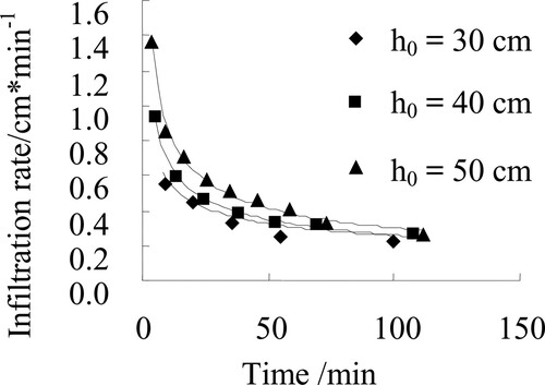
The large differences in soil infiltration rates associated with various head heights are mainly due to the variation in soil-water pressure potential (Cheng et al. 2011; Reynolds 2011). When h₀ = 50 cm, the pressure gradient generated by the infiltration head is the largest, thus resulting in the highest infiltration rate at the soil-water interface. The pressure gradient generated at h₀ = 40 cm is ranked the second, while the pressure gradient at h₀ = 30 cm is the smallest. A similar decreasing trend of soil infiltration rate, going from coarser textured materials to finer textured materials, was shown by Reynolds (2011) and Olson et al. (2013).

Relationship between soil water content change and water movement parameters

Before statistical analysis, several outliers of Δθ from failed tests with backwater are omitted: 3 for h₀ = 30 cm; 4 for h₀ = 40 cm; and 4 for h₀ = 50 cm. Table 1 provides the descriptive statistics of Δθ measured at the 45 test points. Across all the test points, Δθ is less than 15% with a mean of 5.3%. This result indicates that after infiltration, soil water content is increased by 5.3% on average.

Table 1. Descriptive statistics of soil water content before (θ₀) and after (θ_s) infiltration, Δθ = θ_s – θ₀.

	Min	Max	Mean	Variance	Coefficient of variation	Skewness	Kurtosis
θ0	0.216	0.368	0.278	0.034	0.001	0.532	3.221
θs	0.348	0.432	0.392	0.021	0.001	0.452	3.024
Δθ	0.015	0.147	0.053	0.034	0.001	0.954	3.178

Assuming Δθ = 0.01, 0.05, 0.1, 0.15, and 0.2, the head-time curve obtained experimentally at 45 test points is used to estimate 45 values of k_s and ψ, and then the 45 values of each parameter are averaged at h₀ = 30, 40, and 50 cm, respectively (Table 2). The relationship between Δθ and the average of k_s or ψ is analyzed. As Δθ changes from 1% to 20%, k_s decreases by 13%, 12%, and 13%, while ψ increases by 24%, 22%, and 18%, on average, for h₀ = 30, 40, and 50 cm, respectively. These results indicate that the predicted values of the parameters k_s and ψ are pretty much insensitive to Δθ, which is consistent with previous finding of Regalado et al. (2005) and Reynolds (2011).

Table 2. The relationship between soil water content change Δθ and the average values of soil saturated hydraulic conductivity k_s and Green-Ampt wetting front suction ψ.

Δθ	h0 = 30 cm		h0 = 40 cm		h0 = 50 cm
	ks /cm*min^−1	ψ/m	ks /cm*min^−1	ψ/m	ks /cm*min^−1	ψ/m
0.01	0.106	0.09	0.102	0.092	0.071	0.085
0.05	0.104	0.093	0.1	0.096	0.069	0.089
0.10	0.099	0.101	0.096	0.103	0.066	0.093
0.15	0.094	0.107	0.092	0.108	0.064	0.097
0.20	0.092	0.112	0.09	0.112	0.063	0.1

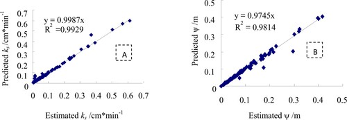
The Δθ values measured at the 45 test points have small standard deviation and are mainly distributed around the mean. The coefficient of variation is around 0.001 (Table 2), indicating a low level of variation. Therefore, the calculation of the parameters k_s and ψ can be simplified by replacing the Δθ measured at different test points by mean Δθ. The relationships between K_s and Ψ values estimated using measured Δθ at every test point and the ones predicted using mean Δθ are shown in Figure 2. The predicted k_s and ψ values are very close to the estimated parameter values, and their linear regression equations are obtained (R² = 0.9929 and 0.9814, respectively). Accordingly, when determining k_s and ψ in large-scale fields, it is not necessary to measure Δθ at all test points (which usually costs massive time and equipment). Instead, mean Δθ can be used to save time and manpower.

Figure 2. The relationships between the parameter values of Ks (A) and Ψ (B) estimated using Δθ measured at every test point and the ones predicted using mean Δθ.

Simplified linear model for solving saturated hydraulic conductivity

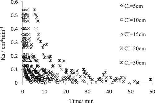
To construct the simplified model for solving k_s, the relationship between k_s and t_i (especially t_med/t_max) is explored. There exists a significant negative correlation between k_s and t_i (p < 0.05). This relationship for h₀ = 30 cm is shown in Figure 3, which confirms that Δθ has little influence on k_s, and the test should therefore focus on the determination of t_i.

Figure 3. The relationship between estimated soil saturated hydraulic conductivity k_s and infiltration time t_i. CI means cumulative infiltration.

As k_s and t_i are negatively correlated, the reciprocal of t_i, namely 1/t_i is taken to facilitate data analysis. The goodness-of-fit between k_s and 1/t_i is tested under specific initial head conditions. Table 3 gives the linear regression coefficients (R²) between k_s and 1/t_i corresponding to different t_i for h₀ = 30, 40, and 50 cm.

Table 3. Linear regression coefficients between soil saturated hydraulic conductivity k_s and the reciprocal of infiltration time 1/t_i.

Infiltration time /min	h0 = 30 cm	h0 = 40 cm	h0 = 50 cm
t5	0.9261	0.8878	0.7226
t10	0.9894	0.9869	0.906
t15	0.9933	0.9484	0.9614
t20	0.9850	0.9938	0.9808
t25	–	0.9902	0.9933
t30	0.9579	0.9903	0.9664
t35	–	–	0.9405
t40	–	0.9313	0.9208
t50	–	–	0.8733

 –, not available.

In the initial stage, the correlation between k_s and t_i is gradually enhanced with increasing infiltration time. However, after R² reaches a certain level, it begins to decrease with increasing time, and the correlation between k_s and t_i is gradually reduced. For h₀ = 30 cm, the reciprocal of the time required for a 15 cm decrease in water level (1/t₁₅) is the best predictor of k_s (R² = 0.9933). For h₀ = 40 and 50 cm, k_s is best predicted by the reciprocal of the time required for a 20 cm decrease in water level (1/t₂₀) and a 25 cm decrease in water level (1/t₂₅; R² = 0.9938 and 0.9933, respectively).

According to the trends of R² with t_i (Table 3), the relationship between k_s and t_i is most evident when half of the water in the tube is infiltrated into the soil. Based on this result, it is not necessary to measure t_max at all test points for field-scale determination of the parameter k_s. As long as t_max is measured at some points to obtain the simplified model, k_s at the other points can be predicted through the model after measurement of t_med. This carries practical implications for saving time, manpower, and material resources in k_s determination in large-area fields.

When controlling for the infiltration time t_i, there are large differences in both the predicted relationship of k_s and 1/t_i for h₀ = 30, 40, and 50 cm. Such differences indicate that h₀ has a strong influence on the prediction performance of the model. Moreover, a poor relationship between k_s and 1/t_i is observed when the test data obtained under all three initial head heights are pooled for parameter prediction. This also indicates that the model’s prediction performance is significantly influenced by h₀. Therefore, to ensure its accuracy, the simplified model for solving k_s must be constructed under constant initial head conditions.

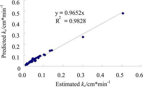
Next, the infiltration data are selected from 30 test points (25 points 1000 m⁻²) out of the 45 points to construct the simplified model for solving k_s, and the model is applied to predict k_s at the remaining 15 test points under every initial head height. The prediction performance of the model is evaluated by fitting the predicted values (y axis) of k_s to the estimated values (x axis). For h₀ = 30 cm, k_s= 0.5411/t_med, the relationship is expressed as: y = 0.9718x (R² = 0.9855). For h₀= 40 cm, k_s= 0.6018/t_med, the relationship is expressed as: y = 1.0655x (R² = 0.9780). For h₀ = 50 cm, k_s= 0.5583/t_med, the relationship is expressed as: y = 0.8978x (R² = 0.9940). The k_s values predicted by the three simplified models are well fitted with all the estimated values (Figure 4). Taken together, the results indicate that the simplified models for solving k_s based on t_med achieve high prediction accuracy and demonstrate potential practical applicability.

Figure 4. The relationship between estimated and predicted values of soil saturated hydraulic conductivity k_s.

Simplified power model for solving Green-Ampt wetting front suction

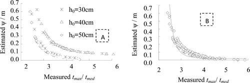
To construct the simplified model for solving ψ, the relationship between ψ and t_i is explored. When h₀ is constant (Figure 5A) or variable (Figure 5B), there is a strong correlation between ψ and t_med/t_max, indicating that h₀ has little influence on ψ. The significant relationship between ψ and t_max/t_med also suggests that Δθ within the range of 0.015–0.147 makes little contribution to ψ in the test soil. Therefore, when determining ψ in large-scale fields, it is not necessary to measure Δθ at all test points, and a large number of ψ values can be obtained directly using the prediction model.

Figure 5. The relationship between estimated Green-Ampt wetting front suction ψ and the ratio of maximum to medium infiltration time t_med/t_max when the initial head height h₀ is constant (A) or variable (B).

To verify the prediction accuracy of the simplified model for solving ψ, the infiltration data are selected from 30 out of the 45 test points (∼25/37.5 points 1000 m⁻²) for model construction, and the constructed model is used to predict ψ at the remaining 15 test points under every initial head height. For h₀= 30 cm, ψ = 120.74*(t_max/t_med)^−5.6933 (R² = 0.9598); the relationship between the predicted values (y axis) and estimated values (x axis) of ψ is expressed as: y = 1.0573x (R² = 0.9985). For h₀= 40 cm, ψ = 87.542*(t_max/t_med)^−5.616 (R² = 0.9775); the relationship is expressed as: y = 0.9532x (R² = 0.9814). For h₀= 50 cm, ψ = 55.894*(t_max/t_med)^−5.4737 (R² = 0.9955); the relationship is expressed as: y = 1.1101x (R² = 0.9952). Overall, the ψ values predicted by the three models are fitted well with the estimated values (R² = 0.9937; Figure 6A). These results indicate that the simplified models for solving ψ based on t_max/t_med achieve high prediction accuracy with practical applicability.

Figure 6. The relationship between estimated and predicted values of Green-Ampt wetting front suction ψ when initial head height h₀ is constant (A) and variable (B).

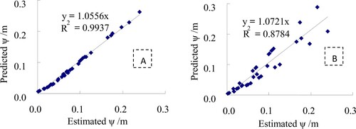
When h₀ is variable, the simplified model also performs well in predicting ψ (Figure 5B), ψ = 63.074*(t_max/t_med)^−5.3735 (R² = 0.9405). The relationship between predicted and estimated values of ψ is expressed as: y = 1.0721x (R² = 0.8784; Figure 6B), which also indicates a relatively high accuracy. This result demonstrates the practical applicability of the simplified model constructed without considering initial head height conditions.

In summary, this study proposes a simplified method for determining the parameters of soil water movement, k_s and ψ, based on Philip-Dunne infiltration tests conducted in a loam soil under field conditions. The results indicate that Δθ within the range of 0.015–0.147 has little influence on k_s or ψ in the test soil, and prediction of the two parameters using mean Δθ meets the accuracy requirements. The proposed method therefore can save time and financial resources by not measuring Δθ at every test point. When determining k_s and ψ in large-scale fields with a homogenous loam soil, t_med and t_max can be measured at a small portion of test points (e.g. 25 / 37.5 points 1000 m⁻²) to construct the models. In particular, k_s can be predicted by the constructed model after measuring t_med alone. The overall sampling rate to characterise the plot is 66.7%. However, this method is useful for field-scale determination of the parameters Ks and Ψ, other than estimating Ks and Ψ at one single point within the field. In addition, the simplified method is only applicable to sites with a single homogeneous soil texture, and the accuracy of the method needs to be further verified with different radii of infiltration tube and soil textures.

Acknowledgments

This study was supported by the National Natural Science Foundation of China [grant numbers 41771256 and 41977087], the Major Scientific and Technological Innovation Projects of Shandong Key R & D Plan (2019JZZY010710), Outstanding Youth Innovation Team in Shandong Province (2020KJF006) and the Major Applied Agricultural Technology Innovation Project in Shandong Province (SD2019ZZ017).

Disclosure statement

No potential conflict of interest was reported by the author(s).

Additional information

Funding

This work was supported by Major Scientific and Technological Innovation Projects of Shandong Key R &amp; D Plan: [grant number 2019JZZY010710]; Major Applied Agricultural Technology Innovation Project in Shandong Province: [grant number SD2019ZZ017]; National Natural Science Foundation of China: [grant number 41771256 and 41977087]; Outstanding Youth Innovation Team in Shandong Province: [grant number 2020KJF006].

Notes on contributors

Junna Sun

Junna Sun, associate professor, Ludong University. The research interest focuses on soil water and salt migration.

Runya Yang

Runya Yang, associate professor, Ludong University. Currently, her research is focused on soil water regulation in aeration drip irrigation.

Mao Yang

Mao Yang, a master student of Ludong University.

Zhenhua Zhang

Zhenhua Zhang, professor, Ludong University, study on the utilization and regulation of regional soil and water resources.

References

- Angelaki A, Sakellariou-Makrantonaki M, Tzimopoulos C. 2013. Theoretical and experimental research of cumulative infiltration. Transp Porous Media. 100(2):247–257.
- Chen CT, Hsu K-C. 2012. Use of falling-head infiltration to estimate hydraulic conductivity at various depths. Soil Sci. 177(9):543–553.
- Cheng Q, Chen X, Chen X, Zhang Z, Ling M. 2011. Water infiltration underneath single-ring permeameters and hydraulic conductivity determination. J Hydrol. 398:135–143.
- De Haro JM, Vanderlinden K, Gomez JA, Giraldez JV. 1998. Medida de la conductividad hidráulica saturada. In: González A., Orihuela D.L., Romero E., Garrido R, editor. Progresos en la Investigación de la Zona No Saturada, Collectanea, vol. 11. Andalusia, Spain: Universidad de Huelva; p. 9–20.
- Derby NE, Korom SF, Casey FXM. 2013. Field-scale relationships among soil properties and shallow groundwater quality. Groundwater. 51(3):373–384.
- Garcıa-Sinovas D, Andrade-Benıtez MA, Regalado-Regalado CM, Alvarez-Benedı J. 2002. Variabilidad espacial de la conductividad hidraulica medida con el permeámetro de Philip–Dunne. In: J. Dafonte et al., editor. Resumenes de las IJornadas sobre Agricultura de Precision. Spain, A Coruna; p. 53–57.
- Gómez J, Giraldez J, Fereres E. 2001. Analysis of infiltration and runoff in an olive orchard under no-till. Soil Sci Soc Am J. 65:291–299.
- Hsu SY, Huang V, Park SW, Hilpert M. 2017. Water infiltration into prewetted porous media: dynamic capillary pressure and Green-Ampt modeling. Adv Water Res. 106:60–67.
- Leung AK, Boldrin D, Liang T, Wu ZY, Kamchoom V, Bengough AG. 2018. Plant age effects on soil infiltration rate during early plant establishment. Geotechnique. 68(7):646–652.
- Liang J, Xing X, Gao Y. 2020. A modified physical-based water-retention model for continuous soil moisture estimation during infiltration: experiments on saline and non-saline soils. Arch Agron Soil Sci. 66(10):1344–1357.
- Lu YZ, Liu PF, Montazar A, Paw UKT, Hu YG. 2019. Soil water infiltration model for sprinkler irrigation control strategy: a case for tea plantation in yangtze river region. Agriculture-Basel. 9(10):260.
- Ma D, Zhang J, Lu Y, Wu L, Wang Q. 2015. Derivation of the relationships between Green–Ampt model parameters and soil hydraulic properties. Soil Sci Soc Am J. 79(4):1030–1042.
- Malama B, Revil A. 2014. Modeling transient streaming potentials in falling-head permeameter tests. Groundwater. 52(4):535–549.
- Mao LL, Li YZ, Hao WP, Zhou XN, Xu CY, Lei TW. 2016. A new method to estimate soil water infiltration based on a modified Green-Ampt model. Soil Tillage Res. 161:31–37.
- Mohammadzadeh-Habili J, Heidarpour M, Khalili D. 2018. Effect of aggregate size and porosity of clay soils on the hydraulic parameters of the Green-Ampt infiltration model. J Hydrol Eng. 23(3):06018001.
- Muñoz-Carpena R, Regalado C, Álvarez-Benedi J, Bartoli F. 2002. Field evaluation of the new Philip-Dunne permeameter for measuring saturated hydraulic conductivity. Soil Sci. 167:9–24.
- MU OZ-CARPENA R, ÁLVAREZ-BENEDI J. WPDUNNE Ver. 1.0. 2002. Available at http://carpena.ifas.ufl.edu (verified 14 Feb. 2005). UF-ITACL, Gainesville, FL and Valladolid, SpainC.
- Olson NC, Gulliver JS, Nieber JL, Kayhanian M. 2013. Remediation to improve infiltration into compact soils. J Environ Manag. 117:85–95.
- Philip JR. 1993. Approximate analysis of falling-head lined borehole permeameter. Water Resour Res. 29(11):3763–3768.
- Réfloch A, Gaudet J-P, Oxarango L, Rossier Y. 2017. Estimation of saturated hydraulic conductivity from ring infiltrometer test taking into account the surface moisture stain extension. J Hydrol Hydromech. 65(3):321–324.
- Regalado CM, Ritter A, Álvarez-Benedí J, Muñoz-Carpena R. 2005. Simplified method to estimate the Green–Ampt Wetting front suction and soil sorptivity with the Philip–Dunne falling-head permeameter. Vadose Zone J. 4:291–299.
- Reynolds WD. 2011. Measuring soil hydraulic properties using a cased borehole permeameter: falling-head analysis. Vadose Zone J. 10:999–1015.
- Reynolds WD. 2013. An assessment of borehole infiltration analyses for measuring field-saturated hydraulic conductivity in the vadose zone. Eng Geol. 159:119–130.
- Sadeghi M, Ghahraman B, Ziaei AN, Davary K, Reichardt K. 2012. Additional scaled solutions to Richards’ equation for infiltration and drainage. Soil Tillage Res. 119:60–69.
- Soil Survey Staff. 1960. Soil classification, a comprehensive system. 7th approximation. Washington: Soil Conservation Service.
- Tsai Y-Z, Liu Y-T, Wang Y-L, Chang LC, Hsu S. 2018. Effects of the grain size on dynamic Capillary pressure and the modified Green–Ampt model for infiltration. Geofluids. 2018:1–11.
- Yang XF, Liu CX, Fang YL, Hinkle R, Li HY, Bailey V, Bond-Lamberty B. 2015. Simulations of ecosystem hydrological processes using a unified multi-scale model. Ecol Modell. 296:93–101.
- Zhang B, Song XF, Zhang YH, Han DM, Tang CY, Yang LH, Wang ZL. 2015. The relationship between and evolution of surface water and groundwater in Songnen Plain, Northeast China. Environmental Earth Sciences. 73(12):8333–8343.
- Zhao J, Xie X, Liu R, Lin C, Gu J, Wang Y, Wang Z. 2019. Comparison of field infiltration test methods for permeable pavement: towards an easy and accurate method. CLEAN – soil, Air. Water. 47(8):1900174.