Spatial variability of soil organic matter and total nitrogen and the influencing factors in Huzhu County of Qinghai Province, China

ABSTRACT

The soil organic matter (SOM) and soil total nitrogen (STN) is a significant concern in Qinghai–Tibet Plateau, China. This study analysed the spatial distribution of SOM and STN and determined their influencing factors to support the conservation of cultivated soil and development of sustainable agricultural strategies in the Plateau. In total, 120 soil samples were collected from the 0–20-cm soil layer in Huzhu County, Qinghai Province. Traditional statistical and geostatistical methods were used to analyse the spatial distribution of SOM and STN; a geographical detector (GeoDetector)was used to explore the factors influencing the spatial variation. The SOM and STN concentrations were 6.92–44.57 and 0.52–2.54 g/kg, respectively. The Cokriging interpolation map showed a similar spatial distribution pattern for SOM and STN concentrations, which decreased from the northeast to southwest directions in the study area. GeoDetector results revealed that the three primary factors influencing the spatial variability of SOM and STN were soil type, annual accumulated precipitation and elevation, with their explanatory power ranging between 38.4% and 59.5%. Two-factor interactions enhanced the explanatory power of the spatial variability of SOM and STN. The research results provide a reference for conservation tillage and precision agriculture.

KEYWORDS:

• Qinghai–Tibet Plateau
• soil organic matter
• soil total nitrogen
• spatial variability
• geodetector
• influencing factor

Introduction

Soil organic matter (SOM) and soil total nitrogen (STN) are two important components of the terrestrial ecosystem and play crucial roles in the global carbon and nitrogen cycling (Knicker et al. 1993; Janzen et al. 1997). Soil carbon storage is 3.3 and 4.5 times greater than that of the atmosphere and biosphere, respectively (Lal 2004); the carbon in the SOM of agricultural ecosystems comprises dominant terrestrial carbon stocks (Huang et al. 2007). In SOM, the average carbon-to-nitrogen ratio is 10:1 (Knicker et al. 1993) and supplies the majority of the nitrogen necessary for plant growth (Knicker et al. 1993; Bingham and Cotrufo 2016). In agricultural ecosystems, SOM and STN indicate soil quality and fertility and are closely associated with the overall soil productivity (Janzen et al. 1997; Ladha et al. 2011). A reduction in the SOM and STN concentrations leads to a decrease in soil fertility and nutrient supply (Falahatkar et al. 2014); this reduction can further influence atmospheric CO₂ concentration as well as global climate change (Tan and Lal 2005). The SOM and STN of cultivated land can be improved through rational use and management in agroecosystems, which could be a huge sink of future atmospheric CO₂ (Jobbágy and Jackson 2000). The role of soils to mitigate climate change by the ‘4 per 1000' concept to increase global SOC stocks by 0.4% has been acknowledged (Dheri and Nazir 2021). An accurate assessment of SOM and STN spatial patterns and it’s influencing factors is a contributor to the rational use and management of cultivated land (Shahriari et al. 2011; Du et al. 2021).

The Qinghai–Tibet Plateau, located at the world’s highest elevation, is known as ‘the Third Pole of the Earth'. The alpine environment of the Qinghai–Tibet Plateau promotes the accumulation of organic carbon during soil formation, and the soil carbon pool of the ecosystem is huge and plays an important role in climate change and global carbon cycle source-sink processes (Wang et al. 2008; Zhao et al. 2012). However, the unique geographical environment is also vulnerable to human activities and climate change. In the context of global warming, the temperature increase rate of the Qinghai–Tibet Plateau is about twice that of the world, which directly affects soil carbon emission processes (Wang et al. 2008; Zhao et al. 2012). In order to understand the feedback effects of soil carbon and nitrogen pools in this region on global climate change, it is necessary to analyse the distribution characteristics of the SOM and STN in the alpine ecosystem and their influencing factors. Previous studies have mainly been conducted in forests, alpine meadows and alpine grassland ecosystems; the results revealed that factors such as grazing (Dai et al. 2021), vegetation degradation (Wu et al. 2020) and climate (Zhao et al. 2018) can have obvious effects on the spatial variability of SOM and STN, which show that the main factors affecting SOM and STN vary between ecosystems and it is necessary to study different ecosystems.

Plateau agriculture developed under the unique climate, soil and water environment of the Tibetan Plateau, is a key part of the region's stability and healthy development (Chen et al. 2021). Although agriculture on the Qinghai-Tibetan Plateau is extremely sensitive to climate change, humans can regulate it by implementing proactive management strategies (Chen et al. 2021). The spatial distribution of SOM and STN is influenced by both structural and random factors, where structural factors refer to natural factors in the formation of the soil (e.g. soil type, topography) and random factors are anthropogenic factors such as land-use practices and cropping systems (Janzen et al. 1997). Several studies conducted in the agricultural ecosystems of other regions have reported that the spatial variability of SOM and STN is influenced by the climate (Li et al. 2019), topography (Ayoubi et al. 2012; Karchegani et al. 2012), soil type (Njeru et al. 2017; Tajik et al. 2020), fertilisation practices (Ladha et al. 2011; Tang et al. 2020), cropping system (Xie et al. 2021) and tillage method (Shahriari et al. 2011). In the corn belt of Northeast China, SOM and STN have been demonstrated to increase with average annual precipitation and decrease with temperature (Li et al. 2019). In Heyang County, southern part of Loess Plateau, topography and soil type are the primary factors influencing the spatial variability of SOM and STN (Chen et al. 2016), whereas in Rugao and Muyang counties, Southeast China, the primary influencing factors are elevation and soil type (Xie et al. 2021). This demonstrates that the spatial variation of SOM and STN as well as their influencing factors can vary across study scales and geographical areas (She and Shao 2009; Xie et al. 2021). Thus, evidence providing targeted information for agricultural management and production in specific regions is both necessary and meaningful (Chen et al. 2016).

Geostatistics, especially kriging, has been used extensively as the analysis methodology for characterising soil spatial variability (Cressie 1990; Azadmard et al. 2018). Several studies have shown that collocating kriging (Cokriging) can significantly improve the interpolation accuracy when the auxiliary variables highly correlate with the unknown variables (Song et al. 2014; Golden et al. 2020). Soil nutrient concentrations are the result of a combination of factors; therefore, Cokriging is widely used in soil nutrient studies and is an effective method for increasing the precision of predictions (Wu et al. 2009; Song et al. 2014). The primary factors that influence soil nutrients vary across regions because of different environments and human activities. Owing to its ability to detect linear and non-linear relationships, as well as interactions based on spatially heterogeneous patterns, geographical detector (GeoDetector) can help explore the factors controlling the concentrations (Du et al. 2021; Liang and Fang 2021). On the basis of the spatial heterogeneity of geographic phenomena, the core idea of GeoDetector is that if geographic factor A is controlled by another geographic factor B, then B will show a spatial distribution similar to that of A (Wang et al. 2016; Wang and Xu 2017). GeoDetector requires the dependent and independent variables to be treated as spatially typed variables, but does not require a linear or non-linear relationship between the dependent and independent variables (Wang and Xu 2017; Du et al. 2021). GeoDetector quantifies the influence of factors on variables, and it has been more and more applied in the field of soil science (Du et al. 2021; Liang and Fang 2021).

In the present study, Huzhu County (CARPC 1984) – an agricultural county located in the Northeastern Qinghai-Tibet Plateau – was selected as the study area. Huzhu County is a typical plateau agricultural region with a long-cultivated history, the cultivated land in Huzhu County covers an area of 773 km², accounting for 1/8 of the total cultivated land in Qinghai Province; wheat, oilseed rape, potatoes and their rotations being the dominant cropping patterns in study area, and the latter two account for 1/4 of Qinghai's production (The People's Government of Huzhu County 2021). According to field surveys, the cultivated land in Huzhu County is cultivated by hand tractors, a cultivation practice that has been maintained for >15 years. Huzhu County is a traditional rain-fed dry farming region with most of the cultivated land is irrigated by natural rainfall, cropping patterns and agricultural management practices are representative of the Tibetan Plateau region (Xu et al. 2019). The present study aimed to (1) characterise the spatial variation of SOM and STN using a combination of classical statistics, geostatistics and geographic information system as well as (2) exploring the factors influencing the spatial variability of SOM and STN.

Materials and methods

The study area

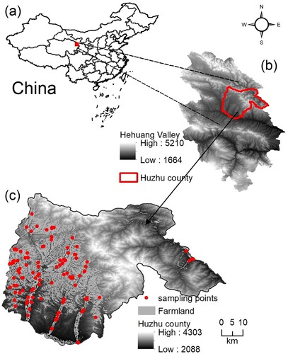
Huzhu County (36°29ʹ–37°10ʹ, 101°46ʹ–102°45ʹ) is located in the northeast of Qinghai Province, China. It has a continental climate with an average annual temperature of 5.8°C and an average annual precipitation of 477.4 mm. This county occupies an area of 3424 km² and has an elevation of 2086–4322 m, of which 733 km² is occupied by cultivated land with an elevation of <3000 m (Figure 1). The Daban Mountains run southeast to northwest through the middle of this county. Regarding topography, Huzhu can be divided into two different natural geographical regions based on the central mountainous areas: the southern and northwestern valleys; several rivers flow from the central high mountain area to both sides. Owing to elevation and topographic changes, major portions of cultivated land are located in mountains with low elevation and river valley flats on the left side of the Daban Mountains. A map of the distribution of cultivated land resources was provided by the Agricultural Technology Extension Centre of Huzhu County (Figure 1).

Figure 1. Location of the study area (a) in Hehuang valley and (b) Hehuang valley. (c) Distribution of soil sampling sites throughout the various topographical features of Huzhu County.

Soil sampling and analysis

Soil samples (depth: 0–20 cm) were collected and stored according to the Technical Specifications for Soil Environmental Monitoring (HJ/T166-2004) (CMEP 2004). Sampling was performed after crop harvesting. Study area were selected to best represent the cultivated area use while considering the terrain attributes and soil type. In total, 120 soil samples were collected. Each sample consisted of 5 soil sub-samples, which were collected the five-point sampling method. All of the sub-samples were collected at a depth of 20 cm, and approximately 500 g of soil was thoroughly mixed to represent as a typical sampling. In order to exclude the effects of fertilisation, soil sampling was conducted at least a week after the crop was harvested. The sampling area details were recorded, including data on geographical coordinates, altitude and soil type. The soil samples were air-dried, passed through a 2-mm sieve and sent to the Testing and Analysis Centre of Qinghai Academy of Agriculture and Forestry Sciences for laboratory analysis. Chemical analysis of the soil was performed according to the following methods: SOM and STN concentrations were determined using the oil bath-K₂Cr₂O₇ titration and semi-micro Kjeldahl methods, respectively (CMEP 2004).

Data preparation

Relief information about surface topography, including slope and aspect, was derived from DEM data of ASTER (http://www.gscloud.cn). True north was used as the reference direction, and the aspect was divided 0°–360° in clockwise direction. According to the calculated angle value, the aspect was divided into five categories: (1) flat ground (−1), (2) sunny slope (135°–225°), (3) half-sunny slope (90°–135° and 225°–270°), (4) half-shady slope (45°–95° and 270°–315°), (5) shady slope (0°–45° and 315°–360°). On the basis of a rural land survey (CARPC 1984), the cultivated land slope was divided into five grades: <2°, 2°–6°, 6°–15°, 15–25°, >25°. Given the relatively large topographic undulations and less cultivated land on steep slopes, the grade categories of 15°–25° and >25° were combined into one single grade such that the cultivated land slope was divided into four grades in total. Soil type data was acquired from the National Geographic Resource Science Subcenter, National Earth System Science Data Centre, National Science &Technology Infrastructure of China (http://gre.geodata.cn), it was geo-referenced and clipped to fit the study area. The soil types of the cultivated land are mainly chernozem – a soil with a deep homogenous humus layer and calcium carbonate leaching sedimentary layer formed under the temperate sub-humid meadow grassland, castnoze – a soil with maroon humus layer and gray-white calcium deposit formed under semi-arid grassland, and meadow soils – a soil with obvious accumulation of humus and rust stained patches formed by diving involved in the process of soil formation. The classification of soil types is based on the Soil Classification System of China, and the name refers to the classification and code for Chinese soil (AQSIQ and SAC 2009).

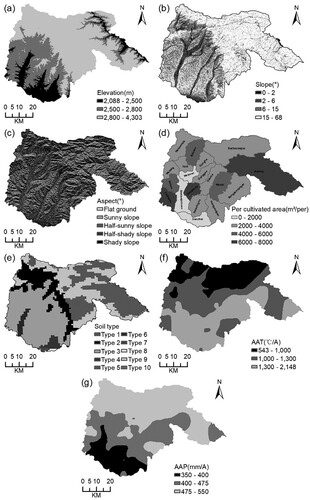
The survey revealed that farming practices were generally consistent across the study area, with crop rotation being the main cropping system, but there were differences in the amount of cultivated land owned by each household. Therefore, the population statistical data of each township in Huzhu County was collected from the 6th National Population Census to calculate the per capita cultivated land area. The annual accumulated precipitation (AAP) and annual cumulative temperature data (AAT) of each township were collected from the Meteorological Bureau of Huzhu City; then, their spatial distribution was established using the Inverse Distance Weighting Method, the two were empirically classified into three categories based on topographic variations. Figure 2 showed the spatial distribution of the seven impact factors.

Figure 2. Spatial distribution of the seven influential factors.

Note: Type 1, cinnamon soils; Type 2, chernozem soils; Type 3, castanozems; Type 4, sierozems; Type 5, litho soils; Type 6, meadow soils; Type 7, fluvo-aquic soil; Type 8, cumulated irrigated soils; Type 9, dark felty soils; Type 10, frigid frozen soils; AAP, annual accumulated precipitation; AAT, annual accumulated temperature.

Statistical and geostatistical analyses

Descriptive statistics and correlation analysis

For SOM and STN, the maximum, minimum, mean, standard deviation, kurtosis, skewness and coefficient of variation (CV) values were calculated to characterise the central trend and spread of the soil parameter datasets. The one-sample Kolmogorov–Smirnov test was used to determine whether the data followed a normal distribution; a suitable transformation was used for non-normally distributed data. Correlations between SOM and STN and influencing factors were also determined. All analyses were performed using IBM SPSS Statistics 24.0.

Cokriging interpolation method

This geostatistical method is based on the theory of regionalised variables and uses semi-variance functions to characterise the spatial variability of regionalised variables (Goovaerts 1999). In geostatistics, semi-variance function parameters (e.g. range, sill and nugget) are used to represent the spatial variability and correlation of regionalised variables on a certain scale; this function also forms the basis for accurate kriging interpolation (Cambardella et al. 1994). The nugget-to-sill ratio can be a criterion for the degree of spatial dependence (DSD) of a variable. DSD is considered strong if it is <25%, moderate if 25%–75% and weak if >75% (Cambardella et al. 1994). The semi-variance function was computed using the following formula: (1) ${\gamma }^{(h)}=\sum _{i=1}^{N^{(h)}}[z(x_i)-z{(x_i+h)}^2]/2N(h)$(1)

where Z(x_i) is the value at location of x_i, h is the lag and N(h) is the number of data pairs separated based on h. Cokriging used in the presence of close correlation between the spatial distribution of specific soil properties and other properties in the same position (Song et al. 2014). The cross-semivariogram is the primary component of Cokriging and serves as an effective tool for evaluating spatial structure and variability (Papritz and Fluhler 1994; Wu et al. 2009). The formula used for cross-semivariogram is as follows: (2) ${\gamma }_{ij}(h)=\sum _{k=1}^{N(h)}\{[z_i(x_k+h)-z_i(x)][z_j(x_k+h)-z_j(x)]\}/2\mathrm{N}(h)$(2)

where γ_ij(h) is the cross-semivariogram of random variables z_i and z_j, h is the separation distance and N(h) is the number of discrete points between z_i and z_j with a given lagged distance interval. The model fitted by the cross-over semi-variance function was selected as the best-fit model with a relatively higher coefficient of determination and smaller residual sum of squares (Wang 1999). The Cokriging method accounts for the correlation among different regional variables; it develops the best valuation method for regionalised variables from a single attribute to two or more coordinated regional attributes, from which estimates can be made to improve the accuracy and rationality of the estimation (Odeh et al. 1995; Song et al. 2014). The following formula is used for the Cokriging prediction model: (3) $Z^{\ast }(x_0)=\sum _{i=1}^N{\lambda }_{1i}{Z}_1(x_i)+\sum _{i=1}^P{\lambda }_{2j}{Z}_2(x_j)$(3)

where Z*(x₀) is the position of the sample point; λ_1i and λ_2j are the weight coefficients assigned to the measured values of the primary and auxiliary variables Z₁ and Z₂, respectively, and N and P are the numbers of measured values of the primary and auxiliary variables Z₁ and Z₂, respectively, involved in the valuation of point x₀. In this study, cross-semivariogram function models between SOM and STN with the auxiliary variables were estimated, and the best-fit model was selected according to the evaluation criteria for the parameters of the semi-variance function theoretical model. Cokriging interpolation was used to predict the SOM and STN concentrations in the study area. The semi-variogram was developed using GS+ version 9.0. ArcGIS 10.6 was used to create the Cokriging interpolation map of variables.

Cross-validation is a common method to validate kriging predictions (Myers 1997). To perform cross-validation, one sample from the dataset was removed and the remaining samples were used for predictions in each iteration; this process was repeated until each sample had been individually removed. The cross-validation indices include mean error (ME), root mean square error (RMSE), mean standard error (MSE), root mean square standardised error (RMSSE) and average standard error (ASE) (Cressie 1990). Moreover, 80% of the training samples were selected as the training set and 20% as the test set by random sampling. This study used the test datasets, which contained 24 reserved sample points, to evaluate the performance of the Cokriging interpolation method. Specifically, the Cokriging interpolation results were assigned to the 24 test sample points to obtain simulation values. A comparative analysis was then performed between the simulation values and the values measured from the 24 test points. ME, RMSE and R² between simulated and measured values were calculated to evaluate the interpolation accuracy (Chai and Draxler 2014).

Geographical detector

The GeoDetector is a spatial heterogeneity detection model (Wang et al. 2016, 2017) used to quantify the driving force of each factor on the dependent variable. The GeoDetector software was downloaded from the website (http://www.geodetector.cn), including the four modules for factor, risk, ecological and interaction detectors. The factor detector can detect whether the independent variable X has an influence on variable Y (e.g. SOM) and can partially explain the spatial differentiation mechanism of variable Y. The factor detector was selected to analyse the driving mechanisms of soil spatial variability, which were assessed using the q-statistic value. The formula for the q-statistic value is shown below. (4) $q=1-{\displaystyle \frac{{\sum }_{h=1}^L{N}_h{\sigma }_h^2}{{N\sigma }^2}q\in [0,1]}$(4)

where q is the explanatory power index of the factors that influence soil spatial variability, wherein the large the value, the greater the explanatory power. When the strata are defined by factor X, q indicates that factor X can explain 100× q% of the spatial pattern. L represents the number of strata. N is the total sample size; N_h is the total number of samples in stratum h; σ and σ² represent the total variance and variance of samples in stratum h, respectively.

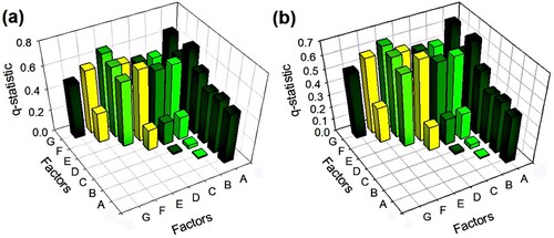
The interaction detector can identify interactions between different influencing factors. X1∩X2 is a new stratum created using a combination of individual factors (X1 and X2); their unique and combination q-statistics are denoted as q(X1) and q(X2) and q(X1∩X2), respectively. Table 1 shows the form of the interaction of two factors according to their relationships. SigmaPlot 10.0 was used to plot the results.

Table 1. Interactions between explanatory variables.

Description	Interaction
q(X1∩X2)<Min(q(X1), q(X2))	Weakened, non-linear
Min(q(X1), q(X2))<q(X1∩X2) <Max(q(X1), q(X2))	Weakened, uni-
q(X1∩X2)>Max(q(X1), q(X2))	Enhanced, bi-
q(X1∩X2)=q(X1)+q(X2)	Independent
q(X1∩X2)>q(X1)+q(X2)	Enhanced, non-linear

Results

Descriptive statistics for SOM and STN

Table 2 outlines the descriptive statistics of SOM and STN. Concentrations of SOM and STN ranged from 6.92 to 44.57 g/kg and 0.52 to 2.54 g/kg with means of 23.41 and 1.53 g/kg, respectively. The variable coefficient of SOM and STN were 35% and 36%, respectively, and were between 25% and 75%; thus, the data had moderate variation (Nielsen and Bouma 1985). An analysis of the probability distribution of the raw SOM data indicated that the distribution exhibited clear deviations; therefore, square root transformation was used to fit a normal distribution. The transformed SOM and raw STN data passed the Kolmogorov–Smirnov test (p < .05), meeting the requirement of geostatistical analysis.

Table 2. Descriptive statistics for SOM and STN.

Variable	Min (g/kg)	Max (g/kg)	Mean (g/kg)	SD	CV (%)	Skew	Kurt	K–S Sig.
SOM	6.92	44.57	23.41	8.25	35	0.46	−0.51	0.005(0.2)^S
STN	0.52	2.54	1.53	0.46	30	0.34	−0.30	0.2^N

Geostatistical analysis results

Identification and treatment of auxiliary variables

Table 3 shows the Spearman correlation coefficients for topography and climate factors correlated with SOM and STN. The correlation between SOM and STN was 0.964. SOM and STN were significantly associated with elevation, AAP and AAT. Elevation showed a significant positive correlation with AAP and a significant negative correlation with AAT. In order to avoid covariance problems caused by strong correlations among elevation, AAP and AAT, principal component analysis was used to extract the main components as auxiliary information. (Jolliffe and Cadima 2016), the first principal component (Factor1) that explained 81% of the total variance was extracted. Factor 1 was then used as an auxiliary variable for the Cokriging interpolation. As a type variable, analysis of variance was used to determine whether the soil type was an auxiliary variable of interpolation. There were significant differences in the concentrations of SOM and STN across soil types (F = 8.764 and F = 9.755, respectively); therefore, soil type was identified as an auxiliary variable. Soil type as a categorical variable required further treatment to be used in the Cokriging interpolation as an auxiliary variable. Therefore, ArcGIS 10.6 was used to overlay the township boundary and soil type maps and calculate the mean values for SOM and STN for the sampling points of the same soil type within the same township; 240 × 240-m mean raster data were generated for SOM and STN based on different soil type and townships (For simplicity of description, these two mean raster data are referred to as ST_som and ST_stn, respectively), replacing the soil type with these two mean raster data as an auxiliary variable for interpolation.

Table 3. Correlation coefficients for SOM, STN and influential factors (*significant at p < 0.05, **significant at p < 0.01).

Variable	STN	Elevation	Slope	Aspect	AAT	AAP
SOM	0.964**	0.427**	−0.076	0.022	−0.598**	0.592**
STN		0.443**	−0.068	0.032	−0.587**	0.558**
Elevation			0.152*	0.035	−0.740**	0.647**
Slope				0.084	−0.118	0.166*
Aspect					−0.098	0.013
AAT						−0.710**

SOM: soil organic matter; STN: soil total nitrogen STN; AAT: annual accumulated temperature; AAP: annual accumulated precipitation.

Semivariogram function analysis for SOM and STN

The semivariogram and spatial variability of SOM and STN were calculated and compared. The semivariogram of soil properties exhibits a good structure, which can be fitted with a Gaussian model (Figure 3). Table 4 presents the Gaussian model parameters for SOM and STN. The SOM variation range of 60,240 m is greater than the STN variation range of 59,830 m, with the two showing correlation over a relatively large range. The DSD values of 16.66% and 16.78% for SOM and STN, respectively, exhibited strong spatial autocorrelation, indicating that their spatial variability is mainly influenced by structural factors.

Figure 3. Semi-variograms of SOM and STN.

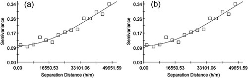
Table 4. Semi-variogram parameters and spatial structures for SOM and STN concentrations.

Variable	Model	Range (m)	C0	C0+C	DSD (%)	R^2	RSS
SOM	Gaussian	60,240	0.35	2.08	16.66	0.97	3.59×10^−2
STN	Gaussian	59,830	0.10	0.59	16.78	0.96	3.50×10^−3

Note: G: Gaussian model; C₀: nugget; C₀+C: sill; DSD: degree of spatial dependence (C₀/[C₀ + C]).

Cokriging interpolation results of SOM and STN

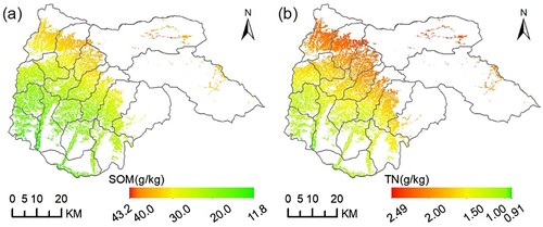
Based on the above correlation analysis results and the optimal semivariogram function model, the STN, factor 1, and ST_stn were used as auxiliary data to perform Cokriging interpolation on SOM, and the STN was performed using SOM, factor 1, and ST_som as auxiliary data. Figure 3 is the Cokriging interpolation map of SOM and STN, and Tables 5 and 6 are the evaluation tables of interpolation accuracy. The cross-validation and the evaluation results between the measured value and the simulated value show that the interpolation result is good (Tables 5 and 6), which can be used to analyse the spatial distribution characteristics of SOM and STN. SOM and STN displayed similar spatial distribution patterns; there was a significant positive correlation (R = .964, P < .01) between the two. Cokriging interpolation map showed a range of 11.79–43.16 and 0.91–2.49 g/kg for SOM and STN concentrations, respectively. A pattern of decreasing SOM and STN concentrations from the northeast to southwest directions in the study area, whereby the higher SOM and STN concentrations were primarily distributed in the northern high-elevation region. According to the national soil nutrient grading standards (NSSO 1998), SOM concentrations in Huzhu County is divided into four grades, accounting for 27.6%, 48.3%, 23.8% and 0.2% of the total cultivated area respectively; the STN concentrations is also divided into four grades, accounting for 0.8%, 38.3%, 42.3% and 18.5% of the total cultivated area respectively (Table 7). The soil nutrient classes were distributed in a graded manner, in general, the nutrient status of STN was better than SOM.

Table 5. Cross-validation of SOM and STN with cokriging interpolation results.

Variable	ME	RMSE	MSE	RMSSE	ASE
SOM	0.00008	0.643	0.00106	1.049	0.6148
STN	0.0011	0.35	0.00454	1.016	0.3471

ME: mean error; RMSE: root mean square error; MSE: mean standard error; RMSSE: root mean square standardised error; ASE: average standard error.

Table 6. Verification between SOM and STN test sets and cokriging interpolation results.

Variable	ME	RMSE	R^2
SOM	2.607	3.489	0.70
STN	0.150	0.204	0.68

Table 7. The statistical results of SOM and TN concentrations for different categories.

SOM				STN
Class	Range (g/kg)	Areas (km^2)	Percentage (%)	Class	Range (g/kg)	Areas (km^2)	Percentage (%)
I	<40	213.8	27.7	I	<2	6.5	0.8
II	40–30	373.3	48.3	II	2–1.5	295.9	38.3
III	30–20	184.3	23.8	III	1.5–1.0	327.3	42.3
IV	20–10	1.6	0.2	IV	1–0.75	143.3	18.5

Spatial variation analysis of SOM and STN based on geodetector

Results of factor detector

The above analysis shows that SOM and STN were mainly influenced by structural factors in study area. Therefore, structural factors such as climate, topography and soil type were selected as influencing factors for detection. It was also found during the field survey that the area of cultivated land per capita varied considerably from township to township, implying different labour inputs in the management of cultivated land, so the area of cultivated land per capita in the township was probed as a random influence factor. Due to software computing power limitations, the SOM, STN and impact factor layers were cropped and converted to a 240*240m raster data, the values of the raster were extracted for calculation.

The factor detector evaluated the explanatory power of seven factors for SOM and STN (Table 8). Soil type, AAP, AAT and elevation were the dominant factors that influenced the spatial variation of SOM and STN. The order of influence (highest to lowest) was as follows: soil type, AAP, AAT and elevation. Other than elevation, which had a slightly greater explanatory power for the spatial variation of STN than SOM, all other factors had similar explanatory power. Changes in the topographical parameters – slope and aspect – had less impact on the spatial variability of the SOM and STN.

Table 8. Factor detector results.

Variation	A	B	C	D	E	F	G
SOM	0.384	0.011	0.015	0.196	0.578	0.286	0.523
STN	0.464	0.012	0.013	0.195	0.595	0.276	0.504

Note: A: elevation; B: elope; C: aspect; D: per cultivated area; E: soil type; F: annual accumulated temperature (AAT); G: annual accumulated precipitation (AAP).

Results of interaction detector

Figure 4 shows the explanatory power of two-factor interactions. The q values of two-factor interaction were higher than those of any individual factor, with the observed effects in the form of binary or non-linear enhancements. The combinations with the greatest explanatory power for spatial variation in SOM and STN were the interaction of soil type with AAP (q = .676) and the interaction of soil type with elevation (q = .692), while being the second most explanatory for each other. The third and fourth combinations were the same in explaining the spatial variation of SOM and STN, i.e. the combination of AAP and elevation, and that of per capita cultivated land of townships and soil types. The results of the interaction detector illustrate the complexity of factor interactions and contribute to a more accurate understanding of the spatial variability of SOM and STN.

Figure 4. Spatial distribution of SOM and STN.

Discussion

SOM and STN spatial pattern characteristics

The study area was a typical agricultural area in the Qinghai–Tibet Plateau region, and the soil nutrients of the cultivated land represent the situation after long-term cultivation. Correlation analysis revealed that SOM and STN increased as AAP increased and AAT decreased. Elevation correlated positively with AAP and negatively with AAT. These results demonstrated that the interaction between climate and elevation can be a dominant factor affecting the spatial distribution of SOM and STN. The geostaistical analysis results showed that SOM and STN had low nugget effects, indicating strong long-range spatial variability. Geostatistical parameters can reflect the spatial dependence of environmental variables (Cambardella et al. 1994). The low nugget effect and relatively strong long-range indicate that the spatial distribution of SOM and STN was primarily influenced by structural factors (Zhu et al. 2018).

From the interpolation results, the distribution pattern of SOM and STN content is more consistent with the trend of elevation change in the study area, gradually decreasing from northeast to southwest. Similar distribution patterns were found in studies in the Taita Mountains of the East African Plateau, where SOM and STN were significantly and positively correlated with elevation change and elevation was an important driver of SOM and STN in mountain ecosystems (Njeru et al. 2017). The high SOM value converges to the SOM concentrations range of 26.0–55.0 g/kg in the eastern Canadian oilseed rape production area (Ma et al. 2015), but compared to the SOM and STN content of 17.8–20.0 and 1.47–1.87 g/kg, respectively, in cultivated land at a similar altitude in the Mexican Plateau study, SOM and STN at relatively low altitude in the study area still have room for improvement and reasonable agricultural management practices are still necessary (Pajares et al. 2009).

Factors influencing the SOM and STN spatial variability

GeoDetector has the potential to measure the consistency of the spatial distribution of two variables (Wang and Xu 2017). The Factor detector results show that the explanatory power of each factor was similar to SOM and STN, likely as a result of the close coupling between SOM and STN in agricultural system. Soil type and climate conditions are the main driving factors for the spatial variation of SOM and STN on a regional scale (Jobbágy and Jackson 2000; Li et al. 2019). Different soil types have different physicochemical properties, which can have a great impact on aeration permeability and fertility retention (Deng et al. 2018), and lead to differences in the ability to store and supply nutrients, this inevitably affects SOM and STN concentrations. In the study area, the main cultivated land soil types were chernozem, castanozem, meadow soils and sierozem, and the distribution of soil type matches, to a certain extent, with gradient change of elevation. Chernozem soil has a high carbon sequestration capacity compared to castanozem soil (Semenov et al. 2008). In this study, when the cultivated soil type is chernozem, the soil nutrient level is mainly level 2, and when the soil type is castanozem soil, the soil nutrient level is mainly level 3 or 4. Figure 2(f,g) demonstrate that the AAP and AAT of the study area show opposite tendencies. In arid areas, water is a limiting factor for crop growth, such that sub-regions with low AAP produce less organic matter (Xin et al. 2016; Du et al. 2021). In contrast, high temperatures promote soil microbial activity and accelerate the depletion of SOM and STN; thus, cool and wet environments are more conducive to the accumulation of soil nutrients (Wang et al. 2017). Topographical factors guide the soil biological and chemical processes and hydrothermal conditions, which closely correlate with the accumulation and decomposition of SOM and STN. In this study, change in the elevation of the cultivated land was higher; with an increase in the elevation, AAP increases gradually and soil moisture conditions improve but AAT decreases, contributing to the accumulation of SOM and STN (Zhu et al. 2018; Kang et al. 2020). Slope and aspect had a small effect on the spatial variability of SOM and STN, which was expected considering the size of the area analysed, variability of climate and high heterogeneity of the soil type. (see Figure 5)

Figure 5. Interaction detector results.

Note: (A) elevation; (B) slope; (C) aspect; (D) per cultivated area of township; (E) soil type; F: annual accumulated temperature; (G) annual accumulated precipitation.

Environmental factors interact with each other to affect the spatial variability of SOM and STN (Wang and Xu 2017; Du et al. 2021). Interaction detector results show that factor interactions enhance the explanatory power of the spatial variation of SOM and STN. The interaction of soil type and other factors has a strong explanatory power for the spatial changes of SOM and STN. When soil characteristics are used as auxiliary factors to predict SOC, the accuracy of the prediction results is improved, which proves the influence of soil characteristics on the spatial variability of SOC (Tajik et al. 2020). The per capita cultivated land of townships ranked fifth in terms of explanatory power as assessed by the factor detector, whereas the interaction q-statistic significantly increased based on the soil type, this may be associated with the fact that soil type shows a certain overlap with the distribution of per capita cultivated land of townships (Figure 2(d,e)). Farming activities destroy the structure of soil aggregates, take away crop residues, and cause changes in SOM (Ajami et al. 2016). The area of cultivated land per capita partly reflect the intensity of farming, and different farming intensities also cause changes in SOM (Li et al. 2019). Regional climate is affected by topographical changes, and topographical attributes affect the decomposition and accumulation of SOM by controlling temperature and moisture (Ajami et al. 2016; Zeraatpisheh et al. 2019). The study area is located on a plateau with great altitude variation, and temperature and rainfall vary significantly with elevation. The dryer and warmer conditions in low altitude areas limit the net primary productivity and carbon input in the soil (Njeru et al. 2017). However, the influence of human activities on cultivated land should not be ignored because agricultural management is an important source of soil nutrients (Li et al. 2019). The geographical orientation of man-made farming management is obvious: the flat terrain in the river valley is convenient for both management and transportation; therefore, the land is used more intensively. Intense agricultural cultivation accelerates soil erosion and organic matter decomposition, causing the cultivated land to have lower SOM concentrations than its potential capacity (Laganière et al. 2010).

Conclusion

We estimated the spatial distribution of SOM and STN in cultivated land in Huzhu County, Qinghai Province. A significant positive correlation was observed between SOM and STN, with similar spatial distribution patterns. SOM and STN concentrations gradually decreased from the northeast to southwest directions of the study area, and fertile cultivated land was mainly distributed in areas with high elevation. The explanatory power of influencing factors was quantified using GeoDetector, wherein soil type, AAP and elevation had strong explanatory power for the spatial variation of SOM and STN, as did two-factor combinations.

Stringent measures should be taken to protect the fertility of cultivated land during agricultural management; the fact that global warming may pose a challenge to the conservation of SOM and STN in this region should also be considered. Conservation tillage and agricultural water engineering facilities should be constructed to improve irrigation in the river valley areas and increase soil nutrient levels. GeoDetector is a powerful tool for exploring the spatial consistency of independent and dependent variables. In this study, this tool explored the factors that influence the spatial variation of SOM and STN while also quantifying their explanatory powers to provide theoretical evidence for the development of strategies for soil nutrient management.

Disclosure statement

No potential conflict of interest was reported by the author(s).

Additional information

Funding

This work was supported by the Second Tibetan Plateau Scientific Expedition and Research Programme (STEP), grant number 2019QZKK0603.

Notes on contributors

Bicheng Zhang

Bicheng Zhang, postgraduate student. Currently working on the study of the land use and its environmental effects.

Lele Niu

Lele Niu, postgraduate student. Currently working on the study of the land use and its environmental effects.

Tianzhong Jia

Tianzhong Jia, postgraduate student. Currently working on the study of the intensive use of cultivated land.

Xiaohua Yu

Xiaohua Yu, is an agronomist at the Agricultural Technology Extension Centre of Huzhu County, Haidong City, Qinghai Pronvince, China. Currently working on soil tillage and farm system.

Diao She

Diao She, professor. He has extensive experience in researching soil environmental effect and ecological restoration.

References

- Ajami M, Heidari A, Khormali F, Gorji M, Ayoubi S. 2016. Environmental factors controlling soil organic carbon storage in loess soils of a subhumid region, northern Iran. Geoderma. 281:1–10. doi:10.1016/j.geoderma.2016.06.017
- [AQSIQ] General Administration of Quality Supervision, Inspection and Qurantine of the People's Republic of China, (SAC)Standardization Administration of China. 2009. Classification and codes for Chinese soil. Beijing. [accessed 2021 Oct 10]. http://c.gb688.cn/bzgk/gb/showGb?type = online&hcno = D59C90AB5DA4F335F0D2BBFE79893627.
- Ayoubi S, Karchegani PM, Mosaddeghi MR, Honarjoo N. 2012. Soil aggregation and organic carbon as affected by topography and land use change in western Iran. Soil Till Res. 121:18–26. doi:10.1016/j.still.2012.01.011
- Azadmard B, Mosaddeghi MR, Ayoubi S, Chavoshi E, Raoof M. 2018. Spatial variability of near-saturated soil hydraulic properties in Moghan plain, North-western Iran. Arab J Geosci. 11. doi:10.1007/s12517-018-3788-8
- Bingham AH, Cotrufo MF. 2016. Organic nitrogen storage in mineral soil: implications for policy and management. Sci Total Environ. 551–552:116–126. doi:10.1016/j.scitotenv.2016.02.020
- Cambardella CA, Moorman TB, Novak JM, Parkin TB., Karlen DL., Turco RF., Konopka AE.. 1994. Field-scale variability of soil properties in central Iowa soils. Soil Sci Soc Am J. 58:1501–1511. doi:10.2136/sssaj1994.03615995005800050033x
- Chai T, Draxler RR. 2014. Root mean square error (RMSE) or mean absolute error (MAE)? – Arguments against avoiding RMSE in the literature. Geosci Model Dev. 7:1247–1250. doi:10.5194/gmd-7-1247-2014
- Chen Q, Yang L, Luo J, Luo J, Liu F, Zhang Y, Zhou Q, Guo R, Gu X. 2021. The 300-year cropland changes reflecting climate impacts and social resilience at the Yellow River-Huangshui River Valley, China. Environ Res Lett. doi:10.1088/1748-9326/abe82a
- Chen T, Chang Q, Liu J, Clevers JGPW. 2016. Spatio-temporal variability of farmland soil organic matter and total nitrogen in the southern Loess Plateau, China: a case study in Heyang County. Environ Earth Sci. 75. doi:10.1007/s12665-015-4786-8
- Chinese Agricultural Regional Planning Committee. 1984. Technical rules for investigation of land use status. Beijing. [accessed 2021 Nov 11]. https://max.book118.com/html/2018/1231/6111142204001242.shtm.
- Cressie N. 1990. The origins of Kriging. Math. Geosci. 22:239–252. doi:10.1007/BF00889887
- Dai L, Fu R, Guo X, Du Y, Lin L, Zhang F, Li Y, Cao G. 2021. Long-term grazing exclusion greatly improve carbon and nitrogen store in an alpine meadow on the northern Qinghai-Tibet Plateau. Catena. 197:104955. doi:10.1016/j.catena.2020.104955
- Deng X, Chen X, Ma W, Ren Z, Zhang M, Grieneisen ML, Long W, Ni Z, Zhan Y, Lv X. 2018. Baseline map of organic carbon stock in farmland topsoil in east China. Agric Ecosyst Environ. 254:213–223. doi:10.1016/j.agee.2017.11.022
- Dheri GS, Nazir G. 2021. A review on carbon pools and sequestration as influenced by long-term management practices in a rice-wheat cropping system. Carbon Manag. 12:559–580. doi:10.1080/17583004.2021.1976674
- Du Z, Gao B, Ou C, Du Z, Yang J, Batsaikhan B, Dorjgotov B, Yun W, Zhu D. 2021. A quantitative analysis of factors influencing organic matter concentration in the topsoil of black soil in northeast China based on spatial heterogeneous patterns. Isprs Int J Geo-Inform. 10. doi:10.3390/ijgi10050348
- Falahatkar S, Hosseini SM, Mahiny A, Ayoubi S, Wang S-Q. 2014. Soil organic carbon stock as affected by land use/cover changes in the humid region of northern Iran. J Mountain Sci. 11:507–518. doi:10.1007/s11629-013-2645-1
- Golden N, Zhang C, Potito A, Gibson PJ, Bargary N, Morrison L. 2020. Use of ordinary Cokriging with magnetic susceptibility for mapping lead concentrations in soils of an urban contaminated site. J Soils Sediments. 20:1357–1370. doi:10.1007/s11368-019-02537-7
- Goovaerts P. 1999. Geostatistics in soil science: state-of-the-art and perspectives. Geoderma. 89:1–45. doi:10.1016/S0016-7061(98)00078-0
- Huang B, Sun W, Zhao Y, Zhu J, Yang R, Zou Z, Ding F, Su J. 2007. Temporal and spatial variability of soil organic matter and total nitrogen in an agricultural ecosystem as affected by farming practices. Geoderma. 139:336–345. doi:10.1016/j.geoderma.2007.02.012
- Janzen H, Campbell C, Ellert B, Bremer E. 1997. Chapter 12 soil organic matter dynamics and their relationship to soil quality. Soil Qual Crop Product Ecosyst Health. 25. doi:10.1016/S0166-2481(97)80039-6
- Jobbágy EG, Jackson RB. 2000. The vertical distribution of soil organic carbon and its relation to climate and vegetation. Ecol Appl. 10:423–436. doi:10.1890/1051-0761(2000)010[0423:TVDOSO]2.0.CO;2
- Jolliffe IT, Cadima J. 2016. Principal component analysis: a review and recent developments. Philos Trans R Soc Math Phys Eng Sci. 374. doi:10.1098/rsta.2015.0202
- Kang X, Li Y, Wang J, Yan L, Zhang X, Wu H, Yan Z, Zhang K, Hao Y. 2020. Precipitation and temperature regulate the carbon allocation process in alpine wetlands: quantitative simulation. J Soils Sediments. 20:3300–3315. doi:10.1007/s11368-020-02643-x
- Karchegani PM, Ayoubi S, Mosaddeghi MR, Honarjoo N. 2012. Soil organic carbon pools in particle-size fractions as affected by slope gradient and land Use change in hilly regions, Western Iran. J Mountain Sci. 9:87–95. doi:10.1007/s11629-012-2211-2
- Knicker H, Frund R, Ludemann HD. 1993. The chemical nature of nitrogen in native soil organic matter. Naturwissenschaften. 80:219–221. doi:10.1007/BF01175735
- Ladha JK, Reddy CK, Padre AT, van Kessel C. 2011. Role of nitrogen fertilization in sustaining organic matter in cultivated soils. J Environ Qual. 40:1756–1766. doi:10.2134/jeq2011.0064
- Laganière J, Angers DA, Paré D. 2010. Carbon accumulation in agricultural soils after afforestation: a meta-analysis. Global Chang Biol. 16:439–453. doi:10.1111/j.1365-2486.2009.01930.x
- Lal R. 2004. Soil carbon sequestration impacts on global climate change and food security. Science. 304:1623–1627. doi:10.1126/science.1097396
- Li X, Shang B, Wang D, Wang Z, Wen X, Kang Y. 2019. Mapping soil organic carbon and total nitrogen in croplands of the Corn Belt of Northeast China based on geographically weighted regression kriging model. Comput Geosci UK. 135:104392. doi:10.1016/j.cageo.2019.104392
- Liang S, Fang H. 2021. Quantitative analysis of driving factors in soil erosion using geographic detectors in Qiantang River catchment, Southeast China. J Soils Sediments. 21:134–147. doi:10.1007/s11368-020-02756-3
- Ma BL, Biswas DK, Herath AW, Whalen JK, Ruan SQ, Caldwell C, Earl H, Vanasse A, Scott P, Smith DL. 2015. Growth, yield, and yield components of canola as affected by nitrogen, sulfur, and boron application. J Plant Nutr Soil Sci. 178:658–670. doi:10.1002/jpln.201400280
- Ministry of Environmental Protection of China. 2004. The technical specification for soil environmental monitoring. Beijing. [accessed 2021 Nov 01]. http://www.doc88.com/p-9783836244048.html.
- Myers, JC.(Van Nostrand Reinhold). (1997). Geostatistical error management. New York: Wiley.
- Nielsen DR, Bouma J. 1985. Soil spatial variability. Wageningen: Pudoc Wageningen. 2–30.
- Njeru CM, Ekesi S, Mohamed SA, Kinyamario JI, Kiboi S, Maeda EE. 2017. Assessing stock and thresholds detection of soil organic carbon and nitrogen along an altitude gradient in an east Africa mountain ecosystem. Geoderma Reg. 10:29–38. doi:10.1016/j.geodrs.2017.04.002
- [NSSO] National Soil Survey Office. 1998. Chinese soil. Beijing: China Agricultural Press.
- Odeh IOA, McBratney AB, Chittleborough DJ. 1995. Further results on prediction of soil properties from terrain attributes – heterotopic cokriging and regression kriging. Geoderma. 67:215–226. doi:10.1016/0016-7061(95)00007-B
- Pajares S, Gallardo JF, Masciandaro G, Ceccanti B, Marinari S, Etchevers JD. 2009. Biochemical indicators of carbon dynamic in an Acrisol cultivated under different management practices in the central Mexican highlands. Soil Till Res. 105:156–163. doi:10.1016/j.still.2009.07.002
- Papritz A, Fluhler H. 1994. Temporal change of spatially autocorrelated soil properties – optimal estimation by Cokriging. Geoderma. 62:29–43. doi:10.1016/0016-7061(94)90026-4
- Semenov VM, Ivannikova LA, Kuznetsova TV, Semenova NA, Tulina AS. 2008. Mineralization of organic matter and the carbon sequestration capacity of zonal soils. Eurasian Soil Sci. 717–730. doi:10.1134/S1064229308070065
- Shahriari A, Khormali F, Kehl M, Ayoubi S, Welp G. 2011. Effect of a long-term cultivation and crop rotations on organic carbon in loess derived soils of Golestan Province, Northern Iran. Int J Plant Prod. 5:147–151.
- She DL, Shao MA. 2009. Spatial variability of soil organic C and total N in a small catchment of the Loess Plateau, China. Acta Agric Scand Sect. B Soil Plant Sci. 59:514–524. doi:10.1080/09064710802425304
- Song G, Zhang J, Wang K. 2014. Selection of optimal auxiliary soil nutrient variables for cokriging interpolation. PLoS One. 9. doi:10.1371/journal.pone.0099695
- Tajik S, Ayoubi S, Zeraatpisheh M. 2020. Digital mapping of soil organic carbon using ensemble learning model in Mollisols of Hyrcanian forests, northern Iran. Geoderma Reg. 20. doi:10.1016/j.geodrs.2020.e00256
- Tan Z, Lal R. 2005. Carbon sequestration potential estimates with changes in land use and tillage practice in Ohio, USA. Agric Ecosyst Environ. 111:140–152. doi:10.1016/j.agee.2005.05.012
- Tang H, Li C, Xiao X, Pan X, Cheng K, Shi L, Li W, Wen L, Wang K. 2020. Effects of long-term fertiliser regime on soil organic carbon and its labile fractions under double cropping rice system of southern China. Acta Agric Scand Sect B Soil Plant Sci. 70:409–418. doi:10.1080/09064710.2020.1758763
- The People's Government of Huzhu County H.C. 2021. Qinghai Province, China, Brief introduction of Huzhu County. Huzhu County.
- Wang G, Li Y, Wang Y, Qingbo W. 2008. Effects of permafrost thawing on vegetation and soil carbon pool losses on the Qinghai-Tibet Plateau, China. Geoderma. 143:143–152. doi:10.1016/j.geoderma.2007.10.023
- Wang J, Xu C. 2017. Geodetector: principle and prospective. Acta Geogr Sin. 72:116–134. doi:10.11821/dlxb201701010
- Wang JF, Zhang TL, Fu BJ. 2016. A measure of spatial stratified heterogeneity. Ecol Indic. 67:250–256. doi:10.1016/j.ecolind.2016.02.052
- Wang S, Adhikari K, Wang Q, Jin X, Li H. 2017. Role of environmental variables in the spatial distribution of soil carbon (C), nitrogen (N), and C:N ratio from the northeastern coastal agroecosystems in China. Ecol Indic. 84:263–272. doi:10.1016/j.ecolind.2017.08.046
- Wang ZC. (Science press). 1999. Geostatistics and its application in ecology (In Chinese). Beijing.
- Wu CF, Wu JP, Luo YM, Zhang L, DeGloria SD. 2009. Spatial estimation of soil total nitrogen using cokriging with predicted soil organic matter content. Soil Sci Soc Am J. 73:1676–1681. doi:10.2136/sssaj2008.0205
- Wu J, Wang H, Li G, Ma W, Wu J, Gong Y, Xu G. 2020. Vegetation degradation impacts soil nutrients and enzyme activities in wet meadow on the Qinghai-Tibet Plateau. Sci Rep UK. 10:21271. doi:10.1038/s41598-020-78182-9
- Xie E, Zhang Y, Huang B, Zhao Y, Shi X, Hu W, Qu M. 2021. Spatiotemporal variations in soil organic carbon and their drivers in southeastern China during 1981–2011. Soil Till Res. 205:104763. doi:10.1016/j.still.2020.104763
- Xin Z, Qin Y, Yu X. 2016. Spatial variability in soil organic carbon and its influencing factors in a hilly watershed of the Loess Plateau, China. Catena. 137:660–669. doi:10.1016/j.catena.2015.01.028
- Xu Q, Song J, Tian H, Zhang Y. 2019. Status of soil nutrients of spring rapeseed panting area and fertilization strategy in eastern Qinghai Province. J Plant Nutr Fertil. 25:157–166. doi:10.11674/zwyf.18040
- Zeraatpisheh M, Ayoubi S, Jafari A, Tajik S, Finke P. 2019. Digital mapping of soil properties using multiple machine learning in a semi-arid region, central Iran. Geoderma. 338:445–452. doi:10.1016/j.geoderma.2018.09.006
- Zhao W, Qi J, Sun G, Li F. 2012. Spatial patterns of top soil carbon sensitivity to climate variables in northern Chinese grasslands. Acta Agric Scand Sect B Soil Plant Sci. 62:720–731. doi:10.1080/09064710.2012.698641
- Zhao Z, Liu G, Mou N, Xie Y, Xu Z, Li Y. 2018. Assessment of carbon storage and its influencing factors in Qinghai-Tibet Plateau. Sustain Basel. 10:1864. doi:10.3390/su10061864
- Zhu J, Wu W, Liu HB. 2018. Environmental variables controlling soil organic carbon in top- and sub-soils in Karst region of southwestern China. Ecol Indic. 90:624–632. doi:10.1016/j.ecolind.2018.03.073