Inverse estimation method for internal defects based on surface stress of carbon-fiber-reinforced plastics using machine learning

Abstract

Carbon-fiber-reinforced plastic (CFRP) is a composite material whose base material is plastic and reinforcement material is carbon fibers. CFRP is widely used in various fields for laminating prepregs. The laminated plate tends to sustain damage, such as delamination, fiber breakage, and base material breakage; hence, we must conduct high-precision and efficient nondestructive testing (NDT). Examples of NDT are ultrasonic examination, X-ray tomography, and infrared stress analysis. With most NDT methods, it is difficult to easily obtain detailed correct information of defects, such as their depth, position, and size. To solve this problem, we develop a machine-learning-aided inverse analysis model that predicts the spatial information of defects from the sum of the principal stresses on the surface calculated from the temperature change measured by infrared analysis, and we propose it as an alternative method to the existing damage analysis. Applying the proposed method to the simulated stress distributions of quasi-isotropic CFRP laminates with defects, the results showed over 99% success to recognize the detail information of defects. Additionally, we examine the properties of the dataset using a forward analysis model and a variational autoencoder. Our method with a convolutional neural network enables us to successfully estimate the information of defects at high speed. Experimental data can be applicable as well as the simulation results to our proposed method, and we believe our method will be a powerful supporting tool for the current NDT for CFRPs.

KEYWORDS:

• machine learning
• non-destructive testing
• finite element method
• carbon-fiber-reinforced plastic
• convolutional neural network
• variational autoencoder

1. Introduction

Carbon-fiber-reinforced plastic (CFRP) is a composite material composed of resin as the base material and carbon fiber as the reinforcing material. Because of its high specific elastic modulus, it is often used in the space and aviation fields. For example, CFRP is used in more than 50% of the airframe structure of the Boeing 787 aircraft [1]. Additionally, this material has high strength and rigidity in one direction. The prepreg, which is a reinforced single-layer board, is commonly used in a stacked configuration [2].

However, damage to the laminated plate is significantly complicated, such as delamination, fiber breakage, and matrix cracking, so it is necessary to analyze damage with high efficiency and accuracy. Damage is generally analyzed through nondestructive testing (NDT) such as ultrasonic measurements [3–9], radiographic transmission [10–13], eddy current testing [14–19], and Lamb wave analysis [20], which require significant labor and time, economic burden, and particularly, experience in radiographic transmission.

In addition to the above existing damage analysis methods, there are methods using infrared thermography [21,22,23–31], and research is also being conducted to improve the accuracy of infrared analysis [4,32].

Infrared thermography is a method of measuring the infrared energy distribution emitted from the surface of an object using an infrared sensor. The measured infrared energy is converted into a temperature distribution. Compared with existing damage analysis methods, this method has the following advantages: there is no need for safety control, the analysis and time costs are low, no contact medium is required, and the skill of the test engineer does not affect the results. Recently, the sum of principal stresses at the surface (DSPSS) is often calculated from the temperature change obtained by infrared analysis, and DSPSS is used in damage analysis. There is a study that confirmed the usefulness of infrared stress analysis of structures for detecting defects in objects such as bridges [33]. The infrared stress analysis is applied to the evaluation of processing damage [34, 35].

On the other hand, research using machine learning has been conducted in addition to damage analysis. Byon et al. divided a CFRP laminate into 10 samples in the longitudinal direction and used the natural frequency and the position and amount of damage as training data in both numerical analysis and experiments, where eight elements, excluding the two elements at the tip, were damaged, and a neural network model was developed. Using this method, they developed a machine learning model to determine the two-dimensional position and amount of damage using the natural frequencies of the first to third orders as input data [36]. In reference [36], the problem they solved was not the prediction of three-dimensional defects. Using conventional machine learning models, it is difficult to handle a high-dimensional data, such as image data and three-dimensional data. However, the deep learning has recently been developed to handle multidimensional data.

On the basis of the above background, in this study, we developed an inverse analysis model that predicts the spatial information of defects, such as size and depth, from DSPSS calculated using the temperature change obtained from infrared analysis. The inverse analysis model employed machine learning to estimate the three-dimensional information of defects from DSPSS directly. Here, it is noted that the data obtained using simulation were used instead of the data obtained by the infrared equipment in this study. We checked the performance of the inverse model we developed. We also investigated the properties of the dataset using a variational autoencoder.

2. Proposed defect inverse estimation method

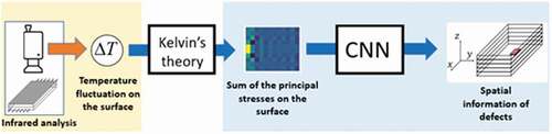
The flow of the proposed defect inverse estimation method is explained in this section and is shown in Figure 1. First, the temperature fluctuations on the surface of the laminated plate are measured by infrared analysis, and DSPSS is derived by applying Kelvin’s theory to the obtained temperature fluctuations. Next, the spatial information of a defect is predicted by the convolutional neural network (CNN) from the obtained DSPSS. The use of CNNs makes it easier to extract features of the input image because it is possible to retain the information of neighboring pixels.

Figure 1. Flow of proposed defect inverse estimation method.

There are two advantages of this model.

1. By using the infrared analysis, one can perform analysis while improving the drawbacks of existing damage analysis methods for the reasons mentioned above.

2. In the inverse analysis that yields a prediction of the structure from DSPSS by a conventional physical simulation, it is necessary to repeat a large amount of forward analysis, which predicts the physical property from the structure, until the objective function converges. On the other hand, by performing inverse analysis using machine learning, one can perform inverse analysis by analyzing only the data necessary for training, which significantly accelerates the estimation of defects.

In this study, DSPSS obtained by numerical analysis was used instead of the data obtained by infrared analysis. There are several advantages to employing data obtained by simulation instead of experiment. First, the preparation of CFRP laminates with defects is very costly. At least 500–700 specimens must be prepared if they are to be used as training data for machine learning. If it is possible to prepare such a large number of specimens, it also takes an excessively long time to obtain the data experimentally for all specimens. In general, measurement errors occur in experiments, whereas data obtained by the numerical analysis do not include measurement errors. The experimental data may include errors due to the measurement environmental conditions, such as temperature and humidity, errors due to the measurement equipment, and noise. If both the experimental data and the numerical results were used from the beginning of this study, it would have been difficult to identify the factors that cause the failure. The exclusion of such errors in the training data makes it easy to verify the proposed inverse model with machine learning. For the proof of the concept of the proposed inverse model with machine learning, we decided to use data from numerical analysis. As the next step, we will work on research based on both the experimental data and the simulation results. In this research, a machine learning model is developed to relate experimental data to simulation results. Therefore, we used the finite element method (FEM) to obtain DSPSS in this study.

The reason why we did not use the infrared transient images obtained by pulse thermography is that pulse thermography involves instantaneous energy transfer from the light source, which is difficult to reproduce by FEM owing to the difficulty in setting the boundary condition. In addition, the temperature distribution is transient. Hence, it is necessary to consider which stage we should use for defect detection. For this reason, we used infrared stress analysis. Note that a fatigue test is required in the infrared stress analysis even though the result is a static stress distribution. For this reason, a careful treatment of the specimen is necessary.

3. Machine learning model

Convolutional neural network (CNN)

The CNN [37] is a special type of neural network used to process data with a grid-like data structure. The term ‘convolutional network’ implies that it uses a mathematical process called ‘convolution’. For example, by convoluting an image such as a handwritten text, it is possible to retain the information of neighboring pixels for learning. In this study, we also use a CNN to convolute DSPSS as image data to estimate the information of defects such as size and depth.

Uniform manifold approximation and projection (UMAP)

UMAP [38] is a method of dimensionality reduction developed from a theoretical framework based on Riemannian geometry and algebraic topology. UMAP visualizes a sequence of points in Euclidean space into a two- or three-dimensional Euclidean space by dimensional compression. In this research, this visualizes the latent variable space obtained by the variational autoencoder (VAE).

VAE

The VAE [39] is a type of generative model that takes the form of a data $x^i$ sampled from a latent variable $z$ that follows a standard normal distribution $N\left(0,1\right)$.

For example, when a handwritten numeric image is used as input, it is known that the numeric labels are located on the standard normal distribution even without providing the numeric label data [40]. In this study, VAE was used for clustering datasets and checking the independence of the dataset.

4. Method

Preparation

In this study, a numerical analysis based on FEM was employed to obtain DSPSS to be used in machine learning. The target CFRP, laminate was designed with unidirectionally reinforced prepregs, as shown in Figure 2(a). In addition, defects of various sizes were included at various depths in the laminate, as shown in Figure 2(b). A total of 2496 laminate models with defects and one laminate model without defects were prepared by changing the spatial position and size of the defects in accordance with the combinations of the ranges as shown in Table 1. The inclusion of the laminate model without defects in the training data improves the accuracy of prediction by the inverse analysis model, especially in the cases of small defects.

Table 1. Defect change conditions.

Length L	10 mm ≤ L ≤ 70 mm, L = 10i (I N)
Width W	10 mm ≤ W ≤ 50 mm, W = 10k (k N)
layer number	Any of the 2nd through 9th layers

Figure 2. (a) Stacking direction of unidirectional reinforcement prepreg and (b) Example dimensions of laminate with defects (red indicates a defect region; white color shows an intact region).

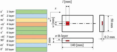
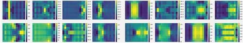
An orthogonal equidistant mesh was used. The intervals of spatial division in the x-, y-, and z-directions were 10, 5, and 0.2 mm, respectively, and the total number of nodes was 990. The prepared laminate model was subjected to tension in the x-direction, as shown in Figure 3, and DSPSS was obtained. In the analysis, the xz plane was symmetrical. The displacement constraint planes were the +yz plane and the -yz plane, and 0.5 mm displacements were applied as tensile deformation. In this study, a defect is represented by changing the properties of the defective part from the values of the CFRP to those of PMMA. In other words, a foreign material is assumed to be contained. The defect size is determined on the basis of [41]. The physical properties of the defective part were expressed using the mechanical properties of acrylic resin (PMMA) of Sumika Acrylic Sales Co [42]. The mechanical properties of CFRP [43] and PMMA are shown in Table 2. By performing numerical calculations under the above conditions, we obtained a dataset that pairs the spatial information of defects with DSPSS of the laminate. Since the results of numerical analysis are normalized and used as the training data for machine learning, the same results are obtained if only the load value changes. However, the prediction by this machine learning model will not be possible if the deformation mode changes, e.g. compression, shear, and tension in different directions from the tensile direction in this study. On the other hand, it is possible to apply this technique to non-uniform stress states such as the distribution around the hole. The results are expected to be obtained by changing the defective part to a hole. Here, a new channel was added to the defect data, as shown in Figure 4. In this additional channel, the value of zero was given if a pixel in the stacking direction was a defect and the value of one was given if the pixel was not a defect. This process allows the sum of the values in the stacking direction to be set to one over the entire the xy plane. Thus, the problem can be solved as a classification problem in the z-direction. In addition, DSPSS was normalized for the entire data set. Figure 5 shows an example of DSPSS.

Table 2. The mechanical properties of CFRP and PMMA (unit of Young’s modulus and shear modulus is MPa).

	E1 [MPa]	E2 [MPa]	E3 [MPa]	12	13	23	G12 [MPa]	G13 [MPa]	G23 [MPa]
CFRP	144700	9650	9650	0.3	0.3	0.45	5200	5200	3400
PMMA	2450	2450	2450	0.39	0.39	0.39	-	-	-

Figure 3. (a) Schematic illustration of analysis condition of FEM, (b) Sample of models (the area surrounded by the red rectangle represents a defect), and (c) DSPSS in FEM.

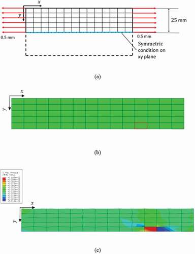
Figure 4. Example of the data of defects used in inverse analysis (red indicates a value of one and white shows a value of zero.).

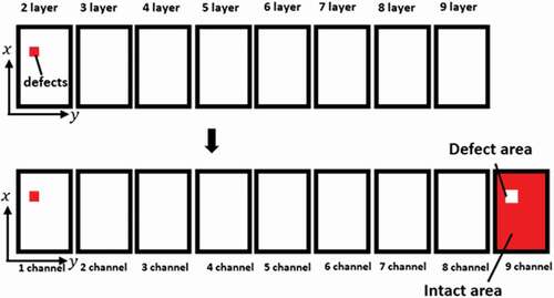
Figure 5. Examples of DSPSS.

Development of CNN to predict spatial information of defects from DSPSS

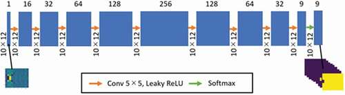
Using the aforementioned dataset, we developed an inverse CNN model to predict the spatial information of defects from DSPSS. The architecture and training process of the CNN are shown in Figure 6. The loss function of CNN is the binary cross entropy, and Adam is used as the optimization method. The classification method for the training data is as follows. For the training data, 1996 pairs were randomly selected from the 2496 pairs of defective datasets, and the remaining 500 pairs were used as the test data. The defect-free dataset was added to the training data. Sixteen images constituted one mini-batch. The training was performed by repeating the evaluation of the loss function and the update of the weights 1000 times. TensorFlow GPU 2.1.0 was used to implement the machine learning model.

Figure 6. Architecture and training process of the CNN.

Evaluation method

The prediction of defects by machine learning was evaluated by visualizing the predicted and simulated defects for 500 pairs of test data.

5. Result

For 497 of the 500 pairs of test data, the test data and the predicted results were in perfect agreement. For the remaining three pairs, the predictions were different from the ground truth (original defect distribution). Figure 7 shows examples of (a) successful and (b) failure prediction. In this study, ground truth is the original defect distribution. A success in this study is defined as the prediction result showing the complete agreement with the ground truth, and the other cases are defined as a failure. In this study, even the three cases of failure are almost identical with the ground truth. The details of these three cases are described below.

Figure 7. (a) Example of 497 pairs of accurate predictions and (b) three pairs of partially failed predictions. The blue region represents the predicted data and the green region represents the ground truth. Purple indicates the defect-free area and yellow indicates the defect area.

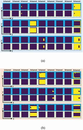
In Figure 7, purple indicates the defect-free area and yellow indicates the defect area. In the first case, a defect exists between the sixth and seventh layers, and its size is 40 mm × 10 mm. One pixel is unsuccessfully predicted (87.5% correct in terms of the area ratio). In the second case, a defect exists between the fourth and fifth layers, and its size is 120 mm × 30 mm. Four pixels are unsuccessfully predicted (94.4% correct in terms of the area ratio). In the third case, a defect is between the fifth and sixth layers, and its size is 110 mm × 40 mm. Two pixels are unsuccessfully predicted (97.7% correct in terms of the area ratio).

6. Discussion

Independence of datasets

The inverse models presented high accuracy for the test data, indicating the possibility that the datasets used in this study are highly independent. The independence of the dataset was examined by observing the latent variable space, which is a low-dimensional representation of the characteristics of defect information and DSPSS using a VAE. Independence here refers to the possibilities that the dataset used in this study has, such as ‘a small defect near the surface and a large defect far from the surface are distinguished by their DSPSSs.’ For the purpose of qualitative analysis of the independence of the datasets, the VAE is developed for DSPSS, and the latent variable space is visualized for discussion.

VAE for DSPSS

Development of VAE

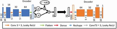
The VAE in DSPSS consists of an encoder to represent DSPSS in low dimensions and a decoder to reproduce the sum of DSPSS from the latent variables represented in low dimensions. A schematic diagram of the VAE for DSPSS is shown in Figure 8. Here, $L_{\mathrm{E}\mathrm{L}\mathrm{B}\mathrm{O}}$ was used as the objective function and Adam was used as the optimization method. The mini-batch size was set to 128. The training was repeated 1500 times. The training data included 2,496 values of DSPSS. The dimensions of latent variable were set as 20. Keras2.4.3 and TensorFlow GPU2.1.0 were used to implement the machine learning model.

Figure 8. Schematic diagram of VAE for DSPSS.

Evaluation of latent variable space

The dimensions of the latent variable required to reproduce DSPSS using the VAE were 20. Here, the latent variable space was visualized by the dimension compression method, UMAP. The groups of data were labeled by color. The results of the layer number where a defect exists, the length of the defect in the x-direction, and the width of the defect in the y-direction are shown in Figures 9–11, respectively. From the figures, the following can be inferred regarding DSPSS. The characteristics of DSPSS can be roughly classified by the layer number where a defect exists.

Figure 9. Latent variable space of DSPSS colored by (a) the layer number of defects (b) length (along x-axis) of defects, and (c) width (along y-axis) of defects.

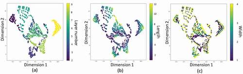
Each group in the figure resembles a triangle. In Figure 9(b), a gradient for each defect length can be seen in all groups. In Figure 9(c), the width of the defect seems to have a weak correlation with the classification of the feature. For the defects in the fourth and seventh layers, and those are in the fifth and sixth layers, their distributions are in the neighborhood of each other. It is considered that the fiber directions are the same in these layers.

7. Conclusion

In this study, we developed a framework for the inverse estimation of internal defects from DSPSS for CFRP laminates using machine learning. The performance of the prediction was verified. In addition, the characteristics of the dataset was investigated using machine learning. As a result, the following points were clarified.

1. The CNN used for the inverse estimation of internal defects from DSPSS is capable of estimating the information of the internal defects, such as their positions and sizes, with high accuracy, i.e. 99.4% accuracy for the test data. This accuracy is defined as the percentage of accurately predicted defect information for 500 test data.

2. The VAE showed that DSPSS used in this study can be classified into features by the layer number where the defect exists.

3. In a low-dimensional form of DSPSS used by the VAE, when the defect information of datasets that were close to each other in the latent variable space, the layer numbers in which defects exist and the shapes of the data are similar.

Disclosure statement

No potential conflict of interest was reported by the author(s).

Additional information

Funding

The author(s) reported that there is no funding associated with the work featured in this article.

References

- Ning FD, Cong WL, Pei ZJ, et al. Rotary ultrasonic machining of CFRP: a comparison with grinding. Ultrasonics. 2016;66:125–132.
- Christensen RM. Mechanics of composite materials. Courier Corporation; 2012.
- Scarponi C, Briotti G. Ultrasonic technique for the evaluation of delaminations on CFRP, GFRP, KFRP composite materials. Compos Part B Eng. 2000;31(3):237–243.
- Zheng K, Chang YS, Wang KH, et al. Improved non-destructive testing of carbon fiber reinforced polymer (CFRP) composites using pulsed thermograph. Polym Test. 2015;46:26–32.
- Mahmoud AM, Ammar HH, Mukdadi OM, et al. Non-destructive ultrasonic evaluation of CFRP–concrete specimens subjected to accelerated aging conditions. NDT E Int. 2010;43(7):635–641.
- Ramanan SV, Bulavinov A, Pudovikov S, et al. (2010, November). Quantitative non-destructive evaluation of CFRP components by sampling phased array. In Proceedings of the International Symposium on NDT in Aerospace, Hamburg, Germany.
- Ibrahim ME, Smith RA, Wang CH. Ultrasonic detection and sizing of compressed cracks in glass-and carbon-fibre reinforced plastic composites. NDT E Int. 2017;92:111–121.
- Lee YJ, Hong SC, Lee JR, et al. Corner inspection method for L-shaped composite structures using laser ultrasonic rotational scanning technique. Adv Compos Mater. 2021;30(5):431–442.
- Mizukami K, Ikeda T, Ogi K. Ultrasonic guided wave technique for monitoring cure-dependent viscoelastic properties of carbon fiber composites with toughened interlaminar layers. Adv Compos Mater. 2021;30(sup2):85–105.
- Sultan MTH, Worden K, Pierce SG, et al. On impact damage detection and quantification for CFRP laminates using structural response data only. Mech Syst Signal Process. 2011;25(8):3135–3152.
- Dilonardo E, Nacucchi M, De Pascalis F, et al. High resolution X-ray computed tomography: a versatile non-destructive tool to characterize CFRP-based aircraft composite elements. Compos Sci Technol. 2020;192:108093.
- Mook G, Pohl J, Michel F. Non-destructive characterization of smart CFRP structures. Smart Mater Struct. 2003;12(6):997.
- Revol V, Plank B, Kaufmann R, et al. Laminate fibre structure characterisation of carbon fibre-reinforced polymers by X-ray scatter dark field imaging with a grating interferometer. NDT E Int. 2013;58:64–71.
- Koyama K, Hoshikawa H, Hirano T (2011, November). Investigation of impact damage of carbon fiber reinforced plastic (CFRP) by eddy current non-destructive testing. In International Workshop Smart Materials, Structures & NDT in Aerospace (pp. 2–4).
- He Y, Tian G, Pan M, et al. Non-destructive testing of low-energy impact in CFRP laminates and interior defects in honeycomb sandwich using scanning pulsed eddy current. Compos Part B Eng. 2014;59:196–203.
- Mook G, Lange R, Koeser O. Non-destructive characterisation of carbon-fibre-reinforced plastics by means of eddy-currents. Compos Sci Technol. 2001;61(6):865–873.
- Wu D, Cheng F, Yang F, et al. Non-destructive testing for carbon-fiber-reinforced plastic (CFRP) using a novel eddy current probe. Compos Part B Eng. 2019;177:107460.
- Xu X, Ji H, Qiu J, et al. Interlaminar contact resistivity and its influence on eddy currents in carbon fiber reinforced polymer laminates. NDT E Int. 2018;94:79–91.
- Yi Q, Tian GY, Malekmohammadi H, et al. New features for delamination depth evaluation in carbon fiber reinforced plastic materials using eddy current pulse-compression thermography. NDT E Int. 2019;102:264–273.
- Voß M, Ilse D, Hillger W, et al. Numerical simulation of the propagation of Lamb waves and their interaction with defects in C-FRP laminates for non-destructive testing. Adv Compos Mater. 2020;29(5):423–441.
- Sakagami T, Kubo S. Applications of pulse heating thermography and lock-in thermography to quantitative nondestructive evaluations. Infrared Phys Technol. 2002;43(3–5):211–218.
- Sakagami T, Kubo S. Development of a new non-destructive testing technique for quantitative evaluations of delamination defects in concrete structures based on phase delay measurement using lock-in thermography. Infrared Phys Technol. 2002;43(3–5):311–316.
- Jinlong G, Junyan L, Fei W, et al. Inverse heat transfer approach for nondestructive estimation the size and depth of subsurface defects of CFRP composite using lock-in thermography. Infrared Phys Technol. 2015;71:439–447.
- Junyan L, Yang L, Fei W, et al. Study on probability of detection (POD) determination using lock-in thermography for nondestructive inspection (NDI) of CFRP composite materials. Infrared Phys Technol. 2015;71:448–456.
- Maier A, Schmidt R, Oswald-Tranta B, et al. Non-destructive thermography analysis of impact damage on large-scale CFRP automotive parts. Materials. 2014;7(1):413–429.
- Marani R, Palumbo D, Renò V, et al. Modeling and classification of defects in CFRP laminates by thermal non-destructive testing. Compos Part B Eng. 2018;135:129–141.
- Swiderski W. Non-destructive testing of CFRP by laser excited thermography. Compos Struct. 2019;209:710–714.
- Popow V, Gurka M. Full factorial analysis of the accuracy of automated quantification of hidden defects in an anisotropic carbon fibre reinforced composite shell using pulse phase thermography. NDT E Int. 2020;116:102359.
- Wu E, Gao Q, Li M, et al. Study on in-plane thermal conduction of woven carbon fiber reinforced polymer by infrared thermography. NDT E Int. 2018;94:56–61.
- Kidangan RT, Krishnamurthy CV, Balasubramaniam K. Identification of the fiber breakage orientation in carbon fiber reinforced polymer composites using induction thermography. NDT E Int. 2021;122:102498.
- Ishikawa M, Hatta H, Habuka Y, et al. Effect of anisotropic properties on defect detection by pulse phase thermography. Adv Compos Mater. 2012;21(1):67–78.
- Chang YS, Yan Z, Wang KH, et al. Non-destructive testing of CFRP using pulsed thermography and multi-dimensional ensemble empirical mode decomposition. J Taiwan Inst Chem Eng. 2016;61:54–63.
- Sakagami T, Izumi Y, Shiozawa D, et al. Nondestructive evaluation of fatigue cracks in steel bridges based on thermoelastic stress measurement. Procedia Struct Integr. 2016;2:2132–2139.
- Muramatsu M, Harada Y, Suzuki T, et al. Infrared stress measurements of thermal damage to laser-processed carbon fiber reinforced plastics. Compos Part A Appl Sci Manuf. 2015;68:242–250.
- Muramatsu M, Nakasumi S, Harada Y. Characterization of defects in carbon fiber-reinforced plastics by inverse heat conduction analysis using transfer matrix between layers. Adv Compos Mater. 2016;25(6):541–555.
- Byon O, Nishi Y. Damage identification of CFRP laminated cantilever beam by using neural network. In: Key engineering materials. Vol. 141. Trans Tech Publications Ltd; 1998. p. 55–64.
- Goodfellow I, Bengio Y, Courville A. Deep learning. MIT Press; 2016.
- McInnes L, Healy J, Melville J (2018). UMAP: uniform manifold approximation and projection for dimension reduction. arXiv preprint arXiv:1802.03426.
- Kingma DP, Welling M. Auto-encoding variational bayes. (2013) arXiv preprint arXiv:1312.6114.
- Jiang Z, Zheng Y, Tan H, et al. (2016). Variational deep embedding: an unsupervised and generative approach to clustering. arXiv preprint arXiv:1611.05148.
- Darabi A, Maldague X. Neural network based defect detection and depth estimation in TNDE. NDT E Int. 2002;35(3):165–175.
- Sumika Acryl Co. Ltd. “SUMIPEX TECHSHEET”. https://www.sumika-acryl.co.jp ( accessed on 3/8/2020).
- Davila C, Camanho P (2003, April). Analysis of the effects of residual strains and defects on skin/stiffener debonding using decohesion elements. In 44th AIAA/ASME/ASCE/AHS/ASC structures, structural dynamics, and materials conference (p. 1465).