Adjustments in the Labor and Real Estate Markets: Estimates of the Time Series Variation in the Natural Vacancy Rate

Abstract

Large similarities exist between the labor and real estate space markets. The natural rate of unemployment (NRU) and the natural vacancy rate (NVR) are important in modeling these markets. The real estate literature has drawn on early modeling of the labor market and has predominantly assumed the NVR to be constant in time. We consider a range of approaches to estimate cross-sectional and time variation in the NVR for the US office market. The results provide no evidence for a time trend, but the NVR may still vary temporally although it is difficult to identify plausible and consistent variation.

Keywords:

• Natural Vacancy Rate
• Natural Rate of Unemployment
• Office Markets

JEL Classification:

• R31
• I1
• I3

Introduction

Research on the workings of real estate space markets has drawn liberally from labor market research. Labor and commercial real estate are inputs into the production of goods and services. They are “owned,” respectively, by workers and landlords. Companies, as employers and tenants, hire workers and pay wages, and lease space and pay rent. A deficiency/surplus in demand means the companies need fewer/more workers and less/more space, leading to increases/decreases in unemployment and in vacant space. The key real estate variables – vacancies, rent and stock of space - correspond to unemployment, wages and the labor force, and the natural vacancy rate (NVR) is a direct analogue of the natural rate of unemployment (NRU).

Other links include asymmetric responses and hidden disequilibrium. The former because of the zero floors on unemployment and vacancies: these variables will respond asymmetrically to positive and negative market shocks (Englund et al., 2008; Hendershott et al., 2010).¹ Negative shocks can lead to large increases in the variables, but positive shocks can only lower the variables so much (and very little if the variables are already very low). The latter arises from the existence of long-term contracts. Demand will depend on historical wage and rent contracts, as well as on new contracts.²

The amount and type of space demanded by firms changes through time owing to changes in production, employment, wage costs and technology. The supply of space also changes as older buildings are demolished, converted or redeveloped and new buildings are constructed. The initial responses to such fundamental changes include adjustments in market rents and the vacancy rate, with both adjusting towards their “natural” or “equilibrium” levels – at which the market will be in full equilibrium (Hendershott, 1996). That is, the differences between actual and natural values drive the adjustments. And since 2002, modeling of adjustment processes has had the equilibrium rent varying over time, depending on levels of demand and supply (e.g., Englund et al., 2008; Hendershott et al., 2013; Hendershott et al., 2002a, 2002b 2010).

The equilibrium or natural vacancy rate (NVR) has generally been assumed to be constant over time but varying across urban areas. However, some of the determinants of differences in cross-section will vary gradually through time as well. While it may be reasonable to assume that the NVR is constant for the periods covered by most modeling, it may not be reasonable for longer horizons. Several authors in the 1980s and 1990s examined time variation in the NVR using a variety of basic approaches (Grenadier, 1995; Sivitanides, 1997; Voith & Crone, 1988) but none produced either a convincing method or particularly plausible results. Our paper makes two contributions. First, we provide a review of labor market studies that focus on the NRU and we show how these studies influenced research on real estate market adjustments and indicate just what this research concluded. Second, we explore a time-varying NVR and make a direct comparison of the different models that appear in the literature, using a common, up-to-date and extensive data set. This means that we are able to focus on results that arise from different modeling approaches as opposed to those that arise from different data sets. We show the difficulties created by all the approaches deployed to model time variation.

The paper has six more sections. The first discusses how the concept of the NRU developed over time and the approaches taken to its estimation. The second explains how the real estate literature adopted labor market concepts and how estimation of the NVR has been undertaken. The third discusses our data, which are for US office markets and include both national level series and panel data for 61 Metropolitan Statistical Areas (MSAs) over 1990–2018 and 18 MSAs over 1980–2018. A fourth sets out the methodology underlying our estimations, while a fifth reports them. We finish with a conclusion and discussion.

Labor Market Studies and the Natural Rate of Unemployment

The concept of the NRU has its origins in the work of Phillips (1958), Samuelson and Solow (1960), Phelps (1967) and Friedman (1968). Posta (2008) reviewed how the concept of the NRU first developed. Phillips (1958) posited a negative relationship between unemployment and wage inflation, which led to the hypothesized trade-off between the two in the form of the Phillips Curve. Then Samuelson and Solow (1960) suggested a negative relationship between unemployment and general price inflation. Phelps (1967) and Friedman (1968) added the expected rate of inflation to the analysis. Phelps (1968), following analysis in Phelps (1967), referred to “the equilibrium employment rate” (p. 682) as existing when actual and expected price inflation are equal and so are actual and expected wage inflation. As a result, Phelps (1968) went on to argue that the equilibrium rate is independent of the rate of inflation. Friedman (1968) referred to this equilibrium as “the natural rate of unemployment” (p. 8).

The related concept of the non-accelerating inflation rate of unemployment (NAIRU) was introduced by Modigliani and Papademos (1975). Nachane (2018) cited Gordon (1997) and Staiger et al. (1997) as examples of writers that use NAIRU and NRU “synonymously” (p. 49). Thirlwall (1983) asserted that “there is no empirical difference between them as they are estimated in the same way” (p. 173), and Ball and Mankiw (2002) argued that “the NAIRU is approximately a synonym for the natural rate of unemployment” (p. 115).

In contrast, Tobin (1997) explained the difference thus:

The NAIRU does not assume … (that) … markets, in particular labor markets, are cleared by existing prices and wages. Instead it assumes an economy in which at any time most markets are characterized by excess demand or excess supply at prevailing prices. … The NAIRU is the employment rate at which the inflation-increasing effects of the excess-demand markets just balances (sic) the inflation-decreasing impacts of the excess-supply markets. Unlike the natural rate, this is a balance among disequilibrium markets, a stand-off between those in excess demand and those in excess supply. (Tobin, 1997, pp. 8–9)

And Claar (2006) stated that “Recent studies have indicated that the terms ‘NAIRU’… and ‘natural rate of unemployment’ are not interchangeable” (p. 2179). He continued: “While NAIRU is an empirical macroeconomic relationship estimated via a Phillips curve, the natural rate is an equilibrium condition in the labor market, reflecting the market’s microeconomic features” (p. 2179). Thus, the NAIRU refers to the relationship between unemployment and inflation and, based on a specific short-run Phillips Curve, is the level of unemployment at which inflation would not increase.³

Most work on the NVR has examined one type of property at either the local or national level in isolation from other types, other investments and other sectors of the economy. In modeling the NVR, no assumptions are usually made of a general equilibrium nor even of equilibrium in all real estate markets. For example, even if the national office vacancy rate were at its natural level and real rental growth were zero, local office markets could be in disequilibrium. Thus, the correct analogue of the NVR would appear to be the NAIRU. Nonetheless, we employ the more commonly used term, NRU, throughout this paper, unless referring to the specific use of an author.

Friedman (1968) emphasized that many determinants of the NRU were institutional and could vary over time. As these variations may be small and slow, Hall (1979) concluded that “fluctuations in the natural unemployment rate are unlikely to contribute much to fluctuations in the observed unemployment rate” (p. 153). He also stated that “Only the costs of recruiting, the costs of turnover to employers, the efficiency of matching jobs and workers, and the cost of unemployment to workers are likely to influence the natural rate of unemployment strongly” (p. 153). We consider similar issues in our discussion of the real estate literature.

Brauer (2007) defined the NRU as “the average unemployment rate that stems from sources other than the business cycle” (p. 2), and Barnichon and Matthes (2017) stated that the NRU is “the hypothetical unemployment rate that is consistent with stable inflation and aggregate production being at its long-run level” (p. 1). Thus, the NRU is identified with specific elements of unemployment, namely structural and frictional unemployment, and not with short-term cyclical fluctuations. There are analogues of both in the real estate market.

Structural reasons for unemployment occur as new industrial sectors emerge and others decline, with the consequence being “a mismatch between workers’ skills or geographic locations and employers’ labor needs” (Daly et al., 2012, p. 4). This may be paralleled in commercial real estate where there is long-term mismatch between space demand and the attributes of available stock, giving rise to obsolescence that may take time to be addressed through conversion or redevelopment. Frictional unemployment arises as workers change jobs, and it exists owing to the imperfect matching process in labor markets (Hall, 1979). Similarly, in real estate markets, there are search costs and delays exist for tenants finding suitable space or for landlords finding tenants.

Most literature on estimating the NRU is derived from the hypothesized inverse relationship between unemployment and wage inflation.⁴ If a constant NRU is included, the relationship is (1) $$w={\beta }_1(u-\mathit{NRU})$$(1) where $w$ is the rate of change in nominal wages, $u$ is the unemployment rate, and ${\beta }_1$ is a constant.⁵

While some studies calculate the NRU directly from the Phillips Curve, most add further variables. A more general form that incorporates partial adjustment to both expected price inflation and the gap between the natural and actual unemployment rate, and includes structural variables is (2) $$w={\beta }_1\left(u-\mathit{NRU}\right)+\alpha E\left(p\right)+\mathit{\beta }\mathit{Z}$$(2) where $E\left(p\right)$ is the expected rate of price inflation, $\mathit{Z}$ is a vector of other relevant variables (such as shocks in rates of change in food and energy prices), $\alpha$ and ${\beta }_1$ are constants and $\mathit{\beta }$ is a coefficient vector. Assuming that the NRU is constant in time, Equations (1)(1) $$w={\beta }_1(u-\mathit{NRU})$$(1) and (2)(2) $$w={\beta }_1\left(u-\mathit{NRU}\right)+\alpha E\left(p\right)+\mathit{\beta }\mathit{Z}$$(2) can be estimated with a constant, ${\beta }_0$ = -${\beta }_1$ NRU, and the estimate of NRU is –${\beta }_0$/${\beta }_1.$

However, Thirlwall (1983) noted the difficulties in estimating the NRU from the “constant term in the equations because the estimates could reflect a mixture of factors and will not be invariant to the pressure of demand” (p. 173). This is also a problem when estimating the NVR.

Blanchard and Katz (1997) proposed and estimated the following model (p. 62): (3) $$w_t={\beta }_0-\beta u_t+p_{(t-1)}-\lambda \left(W_{\left(t-1\right)}-P_{\left(t-1\right)}-Q_{\left(t-1\right)}\right)$$(3)

Thus, wage inflation is explained by the unemployment rate, lagged price inflation, and the gap between the nominal wage level (W) and the sum of the levels of prices (P) and productivity (Q). This is an error correction model (similar to the real estate versions set out in Equations (8)(8) $$\mathit{ln}{RR}_t^{\mathrm{*}}={\lambda }_0+{\lambda }_1\mathit{ln}{D}_t+{\lambda }_{2}ln\left(S_t\right(1-\mathit{NVR}\left)\right)$$(8) and (9)(9) $${rr}_t={\beta }_1\left(v_{t-1}-\mathit{NVR}\right)+{\beta }_2{\mathit{rerr}}_{t-1}+{\beta }_3{d}_t+{\beta }_4{s}_t$$(9) ), with nominal wages adjusting to the gap between actual and natural rates of unemployment (the latter implicit in constant term), and to the gap between the level of actual nominal wages and the equilibrium level (P + Q is the equilibrium nominal wage). Although they do not estimate the natural rate of unemployment, they argue that “the dynamics of the wage equation determine the dynamic effects of variables, such as oil price shocks and payroll taxes, … on the natural rate of unemployment” (p. 65).

The NRU will also vary temporally. Dickens (2009) stated that temporal variation in the NRU goes back at least to Perry (1970), who argued that demographic factors would change the NRU.⁶ Marston (1985) modeled the NRU in MSAs as a national time-varying rate plus a local differential. The unemployment rate is subject to shocks, which create disequilibrium, and part of that persists into the next period, which is also true of the vacancy rate.

The temporal variation depends on the economic environment. For example, when the economy is booming, employers, knowing that replacement could be difficult and costly, could adjust wages to encourage retention; whereas, when the economy is faltering, workers could be disinclined to leave to search for better employment and may accept poorer conditions. Here, the analogy for the real estate market is somewhat tenuous as tenants are the equivalent of employers (both are buyers of inputs into the production process), and workers are the equivalent of real estate owners (both are sellers of inputs into the production process). The power relations, degrees of mobility, costs of mobility and ease of increasing supply will vary substantially between the labor and the real estate markets, and robust data on many of these features of the real estate market do not exist.

Application of Labor Market Research to Estimating the Natural Vacancy Rate

Explanations for the existence of a natural vacancy rate typically refer to the search process that tenants and landlords must undertake to find, respectively, suitable space and occupants (Rosen & Smith, 1983). An additional factor is the desire of landlords to hold an inventory of space to take advantage of changes in market conditions (Shilling et al., 1987). Grenadier (1995) summarized it thus: “The natural vacancy rate is an equilibrium level inventory of space, in the sense that both the matching process between landlord and tenant is facilitated, and that building owners hold an optimal buffer stock of inventory to meet future leasing contingencies” (p. 58). There is no obvious analogue for this in labor economics. The nearest equivalent might be the flexibility of workers to undertake overtime.

Blank and Winnick (1953) were the first to identify the relevance of vacancy rates to rent determination, drawing from the work in labor economics. Rosen and Smith (1983) were the first to link the NVR to the NRU, referring to “The natural or optimal vacancy rate, analogous to the natural unemployment rate…” (p. 780). They stated that “In a manner analogous to the labor market, the housing market requires some normal stock of vacant units to facilitate the search processes of buyers and sellers in the market” (p. 781). They estimated a variant of Equation (2)(2) $$w={\beta }_1\left(u-\mathit{NRU}\right)+\alpha E\left(p\right)+\mathit{\beta }\mathit{Z}$$(2) but with inflation (proxied by the percentage change in operating costs) and no structural variables. In nominal terms, their rental adjustment model was: (4) $$nr=\alpha oe+{\beta }_1\left(v-\mathit{NVR}\right)$$(4) where $nr$ is the rate of nominal rental increase, $\alpha$ and ${\beta }_1$ are positive constants, $oe$ is the rate of change in operating expenses, $v$ is the vacancy rate and$\left(v-\mathit{NVR}\right)$ is the vacancy rate gap.⁷ They suggested that the natural rate could vary in time: “Since this is a cross-sectional model, the rate of interest was not included as an explanatory variable. However, the interest rate could have a significant influence on the cost of vacancies, and hence the natural vacancy rate, over time” (p. 784).⁸

This basic approach, which we term Model A in our following estimations, persisted in the literature until Hendershott (1996) noted a flaw. Starting from equilibrium rents and vacancies, if the vacancy rate rises above its natural level, rents will fall and will continue to do so until the vacancy rate returns to its natural level. While the vacancy rate will be at its natural level, real rent (RR) will be below its equilibrium level, EQRR. For full equilibrium to be attained, Hendershott had real rent adjusting to the deviations of both the vacancy rate and real rent from their natural/equilibrium values. He also allowed for multi-period leases and set his arguments in a rational expectations framework. The addition of the rent gap is analogous to Blanchard and Katz’s (1997) inclusion of the wage gap in Equation (3)(3) $$w_t={\beta }_0-\beta u_t+p_{(t-1)}-\lambda \left(W_{\left(t-1\right)}-P_{\left(t-1\right)}-Q_{\left(t-1\right)}\right)$$(3) : (5) $${rr}_t={\beta }_1\left(v_{t-1}-\mathit{NVR}\right)+{\beta }_2{(RR}_{t-1}-\mathit{EQRR})$$(5)

EQRR was calculated outside the real estate market as the product of replacement cost and the sum of the time-varying real risk-free rate of return, the depreciation rate and the operating expense ratio.⁹ We term this approach Model B. Subsequently, Hendershott et al. (2002) developed an error correction model in which the equilibrium real rent is determined by a reduced form demand-supply equation in levels, and the lagged error term is used in a second stage differences equation for real rental change, which includes adjustment to vacancy and rent disequilibrium and to contemporaneous shocks to demand and supply. This approach was developed by Hendershott et al. (2002a), Englund et al. (2008) and Hendershott et al. (2010) – we term this Model C.

Other research has concentrated on factors that affect either the amount and complexity of search activity or the desirability of maintaining inventories to explain why the NVR will vary from place to place. Gabriel and Nothaft (1988, 2001) distinguished between factors that affect the incidence of vacancy and those that affect the duration that buildings remain empty. For example, a higher level of tenant mobility increases the incidence of vacancy in equilibrium while higher search costs will increase its duration, both of which would lead to a higher NVR.

Zhou (2008), in a study of the Chicago rental housing market from 1994Q1 to 2005Q4, also distinguished between incidence and duration of vacancies. He argued (p. 64) that “incidence is mostly a function of the mobility of the renter population and the rate of new construction” but duration is affected by “the heterogeneity of the vacant rental housing stock,” “the dispersion in rents” and demographic variables.¹⁰

Miceli and Sirmans (2013), in a study of rental housing, use “the theory of efficient wages to explain the natural vacancy rate in rental markets” (p. 20). They explain that “equilibrium unemployment gives workers an incentive to work hard because if they are caught shirking and are fired, they will not immediately be able to find another job and hence will suffer a financial penalty.” They argue that the “equilibrium vacancy rate similarly imposes costs on landlords who fail to maintain their units” because the tenant could leave, and the landlord would lose income. They conclude that high maintenance costs deter expenditure and so require higher levels of rent or greater amounts of vacancy to trigger action by owners. Grenadier (1995) noted how lease structures impact on tenant mobility in office markets.

Factors that increase the cost and complexity of search are likely to lead to higher natural vacancy rates. Arnott and Igarashi (2000) emphasized greater heterogeneity in stock and renters as factors that prolong search. Heterogeneity of stock is higher where there is more variation in the size, age, quality, and location characteristics of buildings available to rent. Related to this, Rosen and Smith (1983) suggested that market size would increase search times and lead to higher NVRs. However, in the context of office markets, Pollakowski et al. (1992) argued that larger markets might be more competitive than smaller ones and less prone to strategic behavior by investors. Meanwhile, Read (1993) discussed whether improvements in market information reduce search costs and lower the NVR.

Hendershott and Haurin (1988) highlighted supply growth, mobility, search factors and holding costs as important influences on natural vacancy rates. Holding costs not only include operating expenses as per Shilling et al. (1987), but also the amount of rent foregone through units remaining empty. Thus, there is an opportunity cost to vacancy that must be assessed at the prevailing discount rate when evaluating the option to wait. Set against this are the possible gains from waiting. Grenadier (1995) noted that anticipated growth in demand would affect the inventory of vacant space that owners wish to hold. Expectations of strong demand growth might encourage owners to wait before leasing and more volatility in demand would increase the option value of holding space vacant. This might be especially marked if leases are long and do not feature escalation clauses.

Many of these factors have been used to explore how the NVR varies across space, but they also suggest that it will vary over time. Demand and supply conditions, expectations and discount rates will all change through time, as will holding costs and factors that affect the ease and costs of search. Some of these factors might change slowly while others might change suddenly because of regulatory or policy decisions. For instance, Vandell (2003) discussed how tax rules and rates might impact NVRs, with the huge changes in US tax rules during the 1980s used as an example. Yet, while clear evidence has been found for cross-section variation in NVRs, empirical results for temporal changes are less convincing.

Wheaton and Torto (1988) added a linear trend to the basic rental adjustment model for the period 1968–86 and concluded that the NVR for US offices had risen by six percentage points in this period. Voith and Crone (1988) applied a variant of the approach used by Marston (1985) to analyze “market-specific natural rates of unemployment” (p. 439). They modeled the vacancy rate in 17 US office markets as the NVR plus a deviation from the natural rate with persistence in the deviation, and they included time fixed effects to consider the common temporal variation in the NVR. The temporal variation from December 1980 to June 1987 was six and a half percentage points. Grenadier (1995) used a different variant of the Marston (1985) approach in a panel of 20 US office markets.¹¹ His results suggested only a single point variation during 1960–91.

Zhou (2008) suggested that the standard assumption of a time-invariant rate “lacks theoretical support” (p. 61). He estimated a model with contemporaneous and lagged values of the vacancy rate and real rental growth and found a single structural break at 2001Q4, which he attributed to a fall in employment following the 9/11 attacks. Zabel (2016, p. 373) developed a model that is “similar in spirit to … models of the natural unemployment rate.” He proposed a model in which vacancies in any period comprise those remaining from the start of the previous period plus vacancies which occurred during the previous period but were not let; and concluded that the vacancy rate would show persistence. He estimated a model with equations for house prices and new supply for a panel for 74 US housing markets, with both adjusting to the lagged vacancy gap. He estimated the NVR using the approach of Gabriel and Nothaft (1988) and modeled the vacancy rate based on the probability of not letting in the previous period. He considered that the NVR could be time-varying but that “estimates of the natural vacancy rate using samples that are dominated by rapid increases or decreases in house prices are not reliable” (p. 386).

Finally, unlike the labor literature, there has been little attempt to incorporate structural variables into models to explain a time-varying NVR. In a study of 24 US office markets during 1980–88, Sivitanides (1997) used structural variables, but the results were poor. He estimated models using either market-specific absorption, change in vacancy rate, completions or employment growth as a structural variable, depending on the statistical fit for each market. He found that temporal variation in the NVR across the sample of MSAs ranged from zero to nearly 28 percent.

Data

The data we use comprise estimates of vacancy rates, rent per square foot per annum, office stock and office-related employment for 61 MSA office markets. The data were provided by CBRE Econometric Advisors and originate from a dataset that was compiled originally by CB Commercial in collaboration with Torto Wheaton Research, as described in Wheaton et al. (1997). Stock and vacancy estimates are based on detailed quarterly surveys by local offices of leasing activity, demolitions, and completions in each market of interest. Records of leases negotiated by CBRE form the basis of the rent series described below. We conduct our analysis using both quarterly and annual frequency observations, with the fourth quarter values of vacancy, rent, stock and employment used in the annual case.

The vacancy rate represents the proportion of stock that is available to let in each market at period end. The stock series on which the vacancy rates are based represent total net rentable area in square feet of what are termed “competitive” multi-tenanted office buildings of at least 20,000 square feet in size. Older buildings that were demolished are removed from the entire series by CBRE Econometric Advisors, meaning that recorded changes in stock from year to year always match additions to stock (that is, completions) recorded for that year, with one exception. Thus, there are no falls in stock in any period for any market in the dataset except for an adjustment to the New York City office stock following the events of 9/11. This adjustment is the minimum value for the stock growth variable shown in Table 1.

Table 1. Summary statistics.

	18 MSAs; 1980–2018					61 MSAs; 1990–2018
	Obs.	Mean	SD	Min	Max	Obs.	Mean	SD	Min	Max
Panel (A): annual
Vacancy rate %	702	14.7	5.3	1	31	1769	14.2	4.5	1.4	29.9
Real rent psf per annum	702	32.2	10.3	15.7	83.2	1769	26.9	9.3	13.5	98.8
Office stock (sq. ft. m)	702	92	63	8.1	313.4	1769	58.2	73.6	4	496.6
Office employment (000 s)	702	416	254	52	1145	1769	276	271	32	1869
Vacancy change	684	0.2	2.6	–6.1	15.3	1708	–0.2	2.2	–7.2	14.9
Real rental growth %	684	–0.5	8	–27.6	47.5	1708	–0.4	7.3	–39	56.6
Stock growth %	684	3.5	4.9	0	35.1	1708	1.7	2	–3.8	16.3
Employment growth %	684	2.6	3.6	–14.7	14.2	1708	2	3.6	–17.4	17.6
Panel (B): quarterly
Vacancy rate %	2754	14.9	5.3	1	31.2	6893	14.3	4.5	0.7	30.1
Real rent psf per annum	2754	32.1	10.2	15.7	85.8	6893	26.9	9.3	13.5	98.8
Office stock (sq. ft. m)	2754	92.2	62.8	8.1	313.4	6893	58.2	73.6	4	496.6
Office employment (000 s)	2754	417	253	52	1145	6893	276	271	32	1869
Vacancy change	2736	0.1	1	–7	9.7	6832	–0.1	0.9	–5.1	4.9
Real rental growth %	2736	–0.2	2.7	–15.8	37.7	6832	–0.1	2.5	–17.1	18.8
Stock growth %	2736	0.9	1.4	0	13.3	6832	0.4	0.7	–4.6	7.4
Employment growth %	2736	0.6	1	–5.8	5.6	6832	0.5	1.1	–7.4	6.6

Note. This table reports summary statistics for the variables used in the modeling of vacancy rates and real rents. Panel (A) is for the annual data and Panel (B) is for the quarterly data. The sections on the left are for the longer time series for 18 Metropolitan Statistical Areas (MSAs) for 1980–2018, and those to the right are for the shorter time series for 61 MSAs for 1990–2018. Sample sizes for rates of change are simply number of MSAs multiplied by number of periods (e.g., 18 MSAs x 38 years = 684 observations). However, sample sizes for variables in levels are higher by one more observation per MSA, reflecting that one further set of observations in levels is needed to compute the rate of change for the first period each time (e.g., 684 annual rates of change + 18 further data points = 702 observations).

Rent indices are constructed by CBRE Econometric Advisors from information on leasing agreements that CBRE was involved with. Nominal rental payments for each lease are summed over the life of the lease contract and then divided by the length of the contract so that the rent figure takes account of any periods of free rent as well as broker commissions. This adjusted rent is divided by the amount of floorspace let and then used as the dependent variable in a hedonic regression that controls for the characteristics of each letting. The model used is set out in Wheaton et al. (1997), who state that the independent variables include the size of the letting and lease length, as well as dummy variables for time, submarket and whether it is a high building, a new building or a gross lease. The reference asset used for index construction is a five-year lease on a gross rent basis for 10,000 square feet in an existing office building. The prediction of this hedonic model of the rent for such a letting in different periods gives a quality-adjusted office rent index for each MSA, which is converted to real terms by CBRE Econometric Advisors using a national consumer price index.¹²

Finally, there are two employment series provided by CBRE Econometric Advisors: financial services and other office-based professional and business services. We sum these to produce a single office employment variable.

Our main period for analysis is 1990 to 2018 for which there is a sample of 61 MSA office markets. We also analyze a subset of 18 markets where there are complete data on all variables of interest over the longer period 1980 to 2018. In both cases, we treated the samples as panel data, and we also created aggregate series for use in national level models. The aggregate series for office employment and office stock were the sum of these variables across the constituent set of markets in each case, while our aggregate series for real rent per square foot per annum and for vacancy rate were stock-weighted averages of the real rent and vacancy series reported for each MSA.

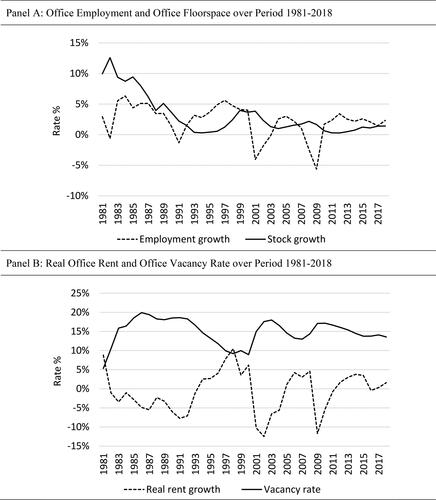
Using the aggregate series for the sample of 18 MSAs, Figure 1 demonstrates the inherent cyclical nature of office markets. Panel (A) plots employment growth and stock growth, and panel (B) plots real rent growth and the vacancy rate. While Panel (B) shows the anticipated inverse relationship between real rent growth and the vacancy rate through time, Panel (A) indicates that both growth in employment and growth in supply have been lower on average since the early 1990s, while employment growth has become more volatile.

Figure 1. Changes in aggregate employment, stock, real rent and vacancy rate. Panel A: Office employment and office floorspace over period 1981–2018. Panel B: Real office rent and office vacancy rate over period 1981–2018.

Note. The graphs are based on aggregate series for the sample of 18 MSAs that have data spanning 1981–2018. Employment and stock were summed across the set of markets, while real rent per square foot per annum and vacancy rate were computed as stock-weighted averages of the series for each MSA in the sample.

Table 1 provides summary statistics for the subset of 18 markets over 1980–2018 and for the full set of 61 MSAs over 1990–2018.

The largest office markets in our sample, whether in terms of stock or employment, are New York, Chicago, Washington DC, Los Angeles and Boston. The maximum values for the stock and employment variables in Table 1 are for New York in 2018. These locations have high per annum rents, but the highest per annum real rent was in San Jose in quarter 4 of 2000. There are some notable outliers in percentage employment growth and percentage stock growth. San Jose had the largest drop in employment (in 2001), the fourth largest drop (in 2002), and one of the largest increases (in 2000), while other large percentage falls in employment occurred in 2008 and 2009 across several markets. The highest rates of stock growth occurred in the 1980s, especially for office markets in Texas, Arizona, Florida and California, while Las Vegas and Orlando recorded large percentage increases in the late 1990s.

The average real rental growth rate is effectively zero. Growth in office employment has been stronger than growth in office stock since 1990, but the reverse is true over the longer horizon. Only thirteen MSA markets have had positive real rental growth over the period 1990–2018. This pattern results from declining rents in the early 1990s, which were largely driven by large scale overbuilding in commercial real estate markets (Hendershott & Kane, 1992) and further falls in the wake of the dot.com bubble and the Global Financial Crisis. Again, there are some notable outliers. San Jose has both the largest annual percentage increase in real rent (56.6% in 2000) and the largest percentage fall (39.0% in 2001). Figures in Table 1 indicate that real rental growth has been much more variable than stock growth or employment growth.

Many of the largest observations for the vacancy rate are in the 1980s, the highest being Houston in quarter 3 of 1987 at 31.2%. The highest vacancy rates post-1990 was in West Beach, FL, in quarter 1, 1993 (30.1%). San Jose recorded the lowest vacancy rate at just 0.7% during quarter 2, 2000. The average change in vacancy rate is close to zero in both the full sample and the subset of office markets, but there are large outliers in Texas and California office markets, with double digit annual changes recorded in some cases. In Houston, the vacancy rate went from 11.6% in 1982 to 26.9% in 1983 (a change of 15.3%), while the largest post-1990 rises were all in 2001 (Austin with a 14.9% rise, San Diego with a 13.1% rise and San Francisco with a 12.3% rise). There are no double digit decreases in either of the samples.

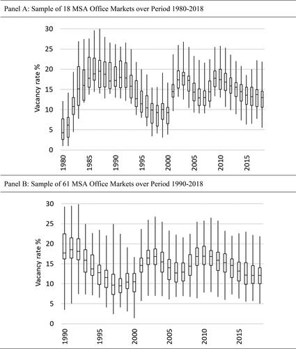
We present an overview of the temporal behavior of vacancy rates in Figure 2. These boxplots show the median vacancy rate in each year as a solid line in the center of each box, the interquartile range in vacancy rates by the box itself, and the full range in vacancy rates in that year by the outer lines. The cyclical nature of real estate occupier markets is evident from these charts, which show both the average rate and typical (inter-quartile) range in rates moving up and down as market conditions change. It is more marked for the subset of 18 locations, which comprises many of the larger MSAs but not New York.¹³ Figure 2 does not suggest an obvious trend through time, but it is noticeable that the cross-section range in the vacancy rate is greater than the temporal range.

Figure 2. Median vacancy rate and dispersion of vacancy rates across MSAs by year. Panel A: Sample of 18 MSA office markets over period 1980–2018. Panel B: Sample of 61 MSA office markets over period 1990–2018.

Note. The box and whisker plots show the interquartile range (spanned by box) and the full range (from minimum to maximum) in recorded office vacancy rates for that year across the sample of MSAs. The horizontal line inside each box indicates the median vacancy rate in the sample that year.

Methodology

Rental Adjustment Models

As we have both annual and quarterly data for two periods, and we have US level and individual MSA data, we use all eight datasets for our analyses. Before considering time variation in the NVR, we estimate models where the $\mathit{NVR}$ is assumed constant. The original rental adjustment model (Model A) is¹⁴ (6) $${rr}_t={\beta }_1\left(v_{t-1}-\mathit{NVR}\right)$$(6) where ${rr}_t$ is real rental growth. The term, $\left(v_{t-1}-\mathit{NVR}\right),$ is the vacancy rate disequilibrium, which causes rents to adjust until real rental growth is zero and the vacancy rate is at its natural rate (NVR). The NVR is unknown and is estimated, as for Equation (2)(2) $$w={\beta }_1\left(u-\mathit{NRU}\right)+\alpha E\left(p\right)+\mathit{\beta }\mathit{Z}$$(2) , from the regression coefficients as $-{\beta }_0/{\beta }_1.$

Next, following Hendershott (1996), we estimate Equation (7)(7) $${rr}_t={\beta }_1\left(v_{t-1}-\mathit{NVR}\right)+{\beta }_2{\mathit{rerr}}_{t-1}$$(7) (Model B). This is a variant of Equation (5)(5) $${rr}_t={\beta }_1\left(v_{t-1}-\mathit{NVR}\right)+{\beta }_2{(RR}_{t-1}-\mathit{EQRR})$$(5) and includes a rent error term so that rents now adjust to both vacancy rate and rent disequilibrium. (7) $${rr}_t={\beta }_1\left(v_{t-1}-\mathit{NVR}\right)+{\beta }_2{\mathit{rerr}}_{t-1}$$(7)

The rent error term is the residual from the long run rent model¹⁵ (8) $$\mathit{ln}{RR}_t^{\mathrm{*}}={\lambda }_0+{\lambda }_1\mathit{ln}{D}_t+{\lambda }_{2}ln\left(S_t\right(1-\mathit{NVR}\left)\right)$$(8) where $\mathit{ln}{RR}_t^{*}$ is the natural logarithm of the time-varying equilibrium real rent, $\mathit{ln}{D}_t$ is the log of demand, which we proxy with employment, and $\mathit{ln}{S}_t$ is log of supply. The rent error is ${\mathit{rerr}}_t=ln{RR}_t-\mathit{ln}{RR}_t^{*},$ where $ln{RR}_t$ is the log of actual real rent.

The final rental adjustment equation (Model C) is within the framework of a conventional Error Correction Model (ECM). The long run model, in log levels, is Equation (8)(8) $$\mathit{ln}{RR}_t^{\mathrm{*}}={\lambda }_0+{\lambda }_1\mathit{ln}{D}_t+{\lambda }_{2}ln\left(S_t\right(1-\mathit{NVR}\left)\right)$$(8) and the short run, adjustment model, in log differences, is (9) $${rr}_t={\beta }_1\left(v_{t-1}-\mathit{NVR}\right)+{\beta }_2{\mathit{rerr}}_{t-1}+{\beta }_3{d}_t+{\beta }_4{s}_t$$(9) where $d_t$ is the rate of growth in demand, $s_t$ is the rate of growth in supply and ${\beta }_3$ and ${\beta }_4$ are constants. Thus, real rents adjust to disequilibrium in real rents and in the vacancy rate, and to contemporaneous shocks to demand and supply, which are the explanatory variables in the long run model.

To consider time variation in the $\mathit{NVR},$ for the single equation versions of these models, we use rolling windows; and, for the panel versions, we include time fixed effects.¹⁶

Time Varying NVR: Models Based on Persistence in the Vacancy Rate

Although the literature on the natural vacancy rate has been dominated by variants of the rental adjustment approach, a separate strand is derived from the model of the persistence of unemployment that was developed by Marston (1985). This model was estimated for a panel but can be used on a single market if rolling windows are used to estimate a time-varying $\mathit{NVR}.$ Substituting $\mathit{NVR}$ for $\mathit{NRU}$ in the Marston specification, the model starts from: (10) $${\mathit{NVR}}_{i,t}={\alpha }_i+{\gamma }_t$$(10) where ${\gamma }_t$ is the NVR in period t and ${\alpha }_i$ is the equilibrium differential for each area, i. The actual rate is the natural rate plus the impact of a shock: (11) $$v_{i,t}={\mathit{NVR}}_{i,t}+{\epsilon }_{i,t}$$(11)

And the effect of a shock is assumed to be persistent: (12) $${\epsilon }_{i,t}=\rho {\epsilon }_{i,t-1}+{\eta }_{i,t}$$(12) where $\rho$ is the persistence, assumed constant across all areas by Marston (1985). Estimates of the $\mathit{NVR}$ and the rate of persistence were derived by using two dates, m periods apart: (13) $$N{VR}_{i,t}={\alpha }_i+{\beta }_t+{\rho }^m(v_{i,t-m}-\mathrm{}{\alpha }_i-{\beta }_{t-m})+{\eta }_{it}$$(13) where ${\eta }_{it}={\sum }_{j=0}^{m-1}{\rho }^j{\eta }_{i,t-j}.$

A variant of this was estimated by Voith and Crone (1988). In their specification, the time-varying component of the natural vacancy rate was included in the persistence process rather than as part of the NVR, and they used time fixed effects. Thus: (14) $$v_{it}={\alpha }_i+{\epsilon }_{it}$$(14) and (15) $${\epsilon }_{it}={\rho }_i{e}_{it-1}+{\gamma }_t+{\mu }_{it}$$(15) giving: (16) $$v_{it}={\alpha }_i\left(1-{\rho }_i\right)+{\gamma }_t+{\rho }_i{v}_{it-1}+{\mu }_{it}$$(16)

A different variant was estimated by Grenadier (1995). In his version, the time-varying component was in the NVR specification, as in Marston (1985): (17) $$v_{it}={\alpha }_i+f_t+{\epsilon }_{it}$$(17) and, rather than time fixed effects, $f_t$ is a fourth order polynomial.

Results

The Rental Adjustment Model

Before examining time variation, we consider whether Models A, B and C produce sensible answers for an NVR that is constant in time. These approaches are well-established in the literature but have never been compared using the same data. If they cannot produce plausible estimates of a time-invariant NVR, they are unlikely to be of value in estimating a time-varying rate. We use both annual and quarterly data and both periods, 1980–2018 and 1990–2018. The results for Equation (6)(6) $${rr}_t={\beta }_1\left(v_{t-1}-\mathit{NVR}\right)$$(6) (Model A) are shown in Table 2, panel (A).¹⁷ The vacancy coefficient is always correctly signed and highly significantly different from zero, and the four estimates of the NVR are in a small range, from 13.6%–14.0%.

Table 2. Rental change models with a constant NVR.

		Dependent variable: Real rental growth
	Sample	1981–2018	1981Q1–2018Q4	1991–2018	1991Q1–2018Q4
	Variable	Coeff.	Coeff.	Coeff.	Coeff.
Panel (A)	Constant	0.09*	0.03***	0.12*	0.04***
		(2.4)	(4.2)	(2.7)	(5.2)
	Lagged vacancy rate	–0.66**	–0.22***	–0.89**	–0.31***
		(–3.1)	(–5.0)	(–3.3)	(–5.6)
	Adjusted R-squared	17.5%	25.4%	15.1%	25.1%
	Implied NVR	13.6%	14.0%	13.6%	13.7%
Panel (B)	Constant	0.06	0.03**	0.11***	0.04***
		(1.4)	(2.9)	(4.1)	(5.4)
	Lagged vacancy rate	–0.49	–0.18***	–0.81***	–0.29***
		(–1.7)	(–3.3)	(–4.1)	(–5.6)
	Lagged rent error	–0.39***	–0.08**	–0.69***	–0.15***
		(–4.8)	(–3.2)	(–8.0)	(–5.4)
	Adjusted R-squared	48.9%	38.7%	76.0%	54.7%
	Implied NVR	13.2%	13.9%	13.5%	13.7%
Panel (C)	Constant	0.11***	0.03***	0.04	0.02
		(5.0)	(7.2)	(0.8)	(1.8)
	Lagged vacancy rate	–0.84***	–0.23***	–0.50	–0.22**
		(–6.7)	(–9.0)	(–1.5)	(–2.9)
	Lagged rent error	–0.21***	–0.04***	–0.66***	–0.13***
		(–4.2)	(–3.4)	(–4.5)	(–3.8)
	Growth in office employment	1.18***	0.98***	0.35	0.52
		(4.8)	(8.1)	(1.0)	(1.9)
	Growth in office stock	–0.54***	–0.43***	1.32	1.03
		(–4.6)	(–3.8)	(1.2)	(1.1)
	Adjusted R-squared	73.8%	57.5%	77.1%	57.1%
	Implied NVR	12.7%	13.1%	8.5%	10.9%

Note. This table reports the results of the estimation of the rental adjustment model set out in Equation (9)(9) $${rr}_t={\beta }_1\left(v_{t-1}-\mathit{NVR}\right)+{\beta }_2{\mathit{rerr}}_{t-1}+{\beta }_3{d}_t+{\beta }_4{s}_t$$(9) .

$${rr}_t={\beta }_1\left(v_{t-1}-\mathit{NVR}\right)+{\beta }_2{\mathit{rerr}}_{t-1}+d_t+s_t$$

where $\mathit{rerr}$ is the residual from the long run model set out in Equation (8)(8) $$\mathit{ln}{RR}_t^{\mathrm{*}}={\lambda }_0+{\lambda }_1\mathit{ln}{D}_t+{\lambda }_{2}ln\left(S_t\right(1-\mathit{NVR}\left)\right)$$(8) .

$$\mathit{ln}{RR}_t^{}={\lambda }_0+{\lambda }_1\mathit{ln}{D}_t+{\lambda }_{2}ln(S_t(1-\mathit{NVR}))$$

In panel (A), only the lagged vacancy rate is used as a regressor; in panel (B), the lagged rent error is added; and in panel (C), the shock variables, growth in office employment and the growth in stock, are added. The dependent variable is the difference in the natural log of the level of real rent, which approximates the rate of growth in real rents. The models are estimated using annual and quarterly data and for 1981–2018 and 1991–2018. These specifications assume that the natural vacancy rate (NVR) is constant in time. All estimations use HAC standard errors and covariances (Bartlett kernel, Newey-West fixed bandwidth = 5.0). The reported test statistics are from t-tests and (^*) indicates significance at 5%; (^**) indicates significance at 1%; and (^***) indicates significance at 0.1%.

We then add the lagged rent error alone, and then with the contemporaneous changes in office employment and in stock (the “shock” variables), as in Equations (7)(7) $${rr}_t={\beta }_1\left(v_{t-1}-\mathit{NVR}\right)+{\beta }_2{\mathit{rerr}}_{t-1}$$(7) and (9)(9) $${rr}_t={\beta }_1\left(v_{t-1}-\mathit{NVR}\right)+{\beta }_2{\mathit{rerr}}_{t-1}+{\beta }_3{d}_t+{\beta }_4{s}_t$$(9) . These results, for Models B and C, are shown in panels (B) and (C). In panel (B), with only the lagged error added, all variables, except the constant and the vacancy rate in the annual model for 1981–2018, are significant. The lagged rent error coefficient in the annual equations is generally a little more than four times that in the quarterly equations, as would be expected with compounding. The coefficients for the shorter sample are about double those for the longer sample, apparently due to differences in time periods and MSA samples. Relative to the estimates without the rent error, the adjusted-R²s are 2.5 and 5 times greater for annual models and a half to double greater for the quarterly models, emphasizing the importance of the rent error. But, crucially, the estimates of the NVR hardly change.

In panel (C), the addition of the shock variables increases the adjusted-R²s substantially for the longer period but only marginally for the shorter period. In the former case, the shock variable coefficients are highly significant; in the latter case they are not. And, for the shorter period, the constant is not significant in either the annual or quarterly models, and the vacancy rate is significant in only the quarterly model. In contrast, the lagged rent error is always highly significant. The estimates of the NVR are reduced by less than a percentage point for the long sample, but by 3% and 5% for the short sample with the insignificant constant. Overall, the models produce plausible and consistent estimates for the national average.

Time Variation in the NVR

Rolling Windows for the Entire U.S.

We now turn to time variation in the NVR, using the national series. We start by considering the three versions of rental adjustment model and estimating rolling windows of 10 years.¹⁸ The results are shown in Figure 3. Two features are apparent:¹⁹

Figure 3. Estimates of the natural vacancy rate from the short run rent model using rolling 10-year windows. Panel A: Sample of 18 MSAs for windows ending 1990–2018, annual LHS and quarterly RHS. Panel B: Sample of 61 MSAs for windows ending 2000–2018, annual LHS and quarterly RHS.

Note. Model A is the traditional rental adjustment model shown in Equation (6)(6) $${rr}_t={\beta }_1\left(v_{t-1}-\mathit{NVR}\right)$$(6) . Model B adds the residual error from Equation (7)(7) $${rr}_t={\beta }_1\left(v_{t-1}-\mathit{NVR}\right)+{\beta }_2{\mathit{rerr}}_{t-1}$$(7) to the specification of Model A. While we also estimated Equation (8)(8) $$\mathit{ln}{RR}_t^{\mathrm{*}}={\lambda }_0+{\lambda }_1\mathit{ln}{D}_t+{\lambda }_{2}ln\left(S_t\right(1-\mathit{NVR}\left)\right)$$(8) , a short run rent model that includes shock variables, estimates of the natural vacancy rate based on this are unstable so are not shown. In each case, the NVR is estimated from the regression coefficients as –β₀/β₁.

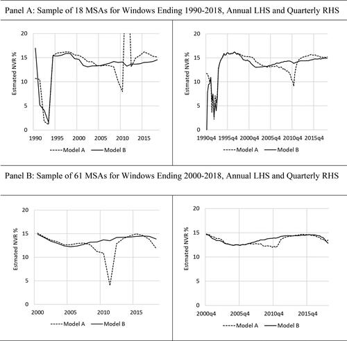
• in some periods the NVR estimate is ridiculous because the constant or the vacancy rate coefficient is very small, which is a common problem in such estimations; and

• the prevailing time variation is consistent across the models, with gentle cycles between 13% and 16%, and peaks around 1998 and 2009, troughs around 2002 and 2011, and a gradual rise thereafter, although the shorter period models suggest a gentle fall around 2017. There is no evidence of a secular trend.

Error Correction Model

Next, we use the panel data sets, with which we can use time fixed effects to derive estimations of the time variation in the NVR from the ECM models. First, as a sense check, we consider the cross-section MSA estimates of the NVR from the three rental adjustment models. The MSA figures are summarized in Table 3. The means and standard deviations are very similar for both periods and for all models, and the lowest correlation is 0.85. The correlations with the actual time series averages for the MSAs are also high. These results suggest that the models are all capturing the same cross-section differences and again point to a robustness in this approach for MSA variation.

Table 3. Cross-section variation in the NVR from the short run ECM models.

	1981–2018		1981Q1–2018Q4		1991–2018		1991Q1–2018Q4
	Mean and standard deviation
Panel (A)	Mean	SD	Mean	SD	Mean	SD	Mean	SD
Model A	12.5%	2.3%	13.4%	2.3%	12.0%	4.0%	12.7%	3.2%
Model B	13.5%	2.3%	13.9%	2.4%	12.6%	3.2%	12.9%	3.0%
Model C	10.7%	2.1%	12.6%	2.2%	11.3%	2.7%	12.1%	2.8%
Panel (B)	Correlations between models
	Model A	Model B	Model A	Model B	Model A	Model B	Model A	Model B
Model B	93.2%		99.1%		97.7%		99.6%
Model C	85.1%	88.5%	97.8%	98.3%	88.7%	93.0%	98.2%	98.9%
Panel (C)	Correlations with actual average
Model A	77.6%		91.3%		60.9%		73.4%
Model B	95.0%		96.0%		75.9%		79.2%
Model C	82.7%		93.4%		82.3%		81.1%

Note. This table presents summary statistics for the NVR estimates from panel versions, with MSA and time fixed effects, of the three real rental growth models presented in Table 2. Model (A) includes only the lagged vacancy rate; model (B) adds the lagged rent error; and model (C) adds the shocks variables – growth in office employment and growth in stock. The models are estimated using annual and quarterly data and for 1981–2018 and 1991–2018. For each model, the mean and standard deviation of the cross-section estimates of the MSA natural vacancy rates are presented and, below these, are the correlations among the models. The means and standard deviations are given in percentages. The correlations with the actual averages are for the time series averages for each MSA.

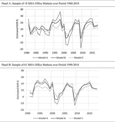
Figure 4 shows the time fixed effects for the three rental adjustment models. The results are remarkably consistent across models and panels. While the series have averages in the 10.5–14.0% range, the variations around this are large, with significant periods above 20% and below 5%, and all models have some negative estimates. The range of the variations falls as additional variables are added but the estimates are always too volatile. The estimates of the NVR suffer from sensitivity to small changes in the small magnitudes of the estimated coefficients and the time fixed effects. The linear trends are gently upward for the longer period and very gently downwards for the shorter period.

Figure 4. Estimates of the natural vacancy rate based on time fixed effects in a short run rent model, annual data. Panel A: Sample of 18 MSA office markets over period 1980–2018. Panel B: Sample of 61 MSA office markets over period 1990–2018.

Note. Model A is the traditional rental adjustment model shown in Equation (6)(6) $${rr}_t={\beta }_1\left(v_{t-1}-\mathit{NVR}\right)$$(6) . Model B adds the residual error from Equation (7)(7) $${rr}_t={\beta }_1\left(v_{t-1}-\mathit{NVR}\right)+{\beta }_2{\mathit{rerr}}_{t-1}$$(7) to the specification of Model A. Model C adds shock variables and is shown in Equation (8)(8) $$\mathit{ln}{RR}_t^{\mathrm{*}}={\lambda }_0+{\lambda }_1\mathit{ln}{D}_t+{\lambda }_{2}ln\left(S_t\right(1-\mathit{NVR}\left)\right)$$(8) . All three models include time and MSA fixed effects. The results from estimation of these models on quarterly frequency data show the same general pattern. Because they are much noisier, they are not shown.

Persistence Models

Next, we consider persistence models derived from Equations (10)–(17). First, we present the results for models for the whole U.S. and then for models using the four sets of panel data.

Models for the Entire U.S.

Table 4 shows the results for estimates of constant NVR and persistence from the models of Marston (1985), Voith and Crone (1988) and Grenadier (1995). With the exception of the Grenadier (1995) model, the NVR estimates are sensible, consistent with estimates from previous analysis and are lower for the shorter period. The Grenadier estimates are always higher and, in one case, implausibly high. The estimates of persistence are, not surprisingly, much higher for the quarterly data.

Table 4. Estimates of the NVR from persistence models for whole US.

		1981–2018	1981Q1–2018Q4	1991–2018	1991Q1–2018Q4
Voith and Crone	NVR	15.6%	16.3%	13.0%	11.8%
	Persistence	0.76	0.96	0.80	0.98
Marston (m = 3)	NVR	15.3%	15.9%	13.5%	12.9%
	Persistence	0.44	0.94	0.33	0.95
Grenadier	NVR	16.3%	68.9%	25.1%	24.1%
	Persistence	0.72	0.98	0.63	0.95

Note. This table presents the results of three types of persistence models used to estimate the NVR, from Marston (1985), Voith and Crone (1988) and Grenadier (1995). The figures are for estimates of the persistence of a shock to the vacancy rate and the implied NVR. All models are estimated using US level data and so produce a single national estimate of the NVR. The models are estimated using annual and quarterly data and for 1981–2018 and 1991–2018. Without a time-varying NVR, the Voith and Crone annual model is the Marston model with a lag of one year (m = 1). For the quarterly Voith and Crone model, we use a lag of one quarter. For the Marston model, after a three-period lag (m = 3), the persistence estimates are very close to one, so the NVR estimates are very large and are not presented. The NVR estimates are given as percentages.

The Marston and the Voith and Crone models use time fixed effects, so time-variation in these models requires a panel. In contrast, the Grenadier model uses a fourth-degree polynomial for the time trends, so could be estimated using U.S. level data. To avoid unnecessary duplication, we report only the panel results.

Panel Models

We start with cross-section estimates of the NVR in the MSAs. Table 5 shows the means and standard deviations of the cross-section estimates from the models of Voith and Crone (1988), Marston (1985), and Grenadier (1995).

Table 5. Estimates of the NVR from persistence models using panel models.

	1981–2018		1981Q1–2018Q4		1991–2018		1991Q1–2018Q4
Panel (A): Marston	m = 4	m = 3	m = 4	m = 3	m = 4	m = 3	m = 4	m = 3
Estimates of MSA NVRs
Mean	15.4%	15.6%	15.5%	15.6%	13.5%	13.4%	13.6%	13.5%
SD	2.8%	2.8%	2.7%	2.8%	2.3%	2.3%	2.3%	2.3%
Correlation with quarterly	99.9%	99.9%			99.9%	99.9%
Correlation with actual average	99.2%	99.2%	99.1%	99.2%	97.4%	97.0%	97.5%	97.2%
Persistence
Common	0.70	0.73	0.91	0.92	0.61	0.69	0.88	0.91
Panel (B): Voith & Crone			Persistence
	Com.	MSA	Com.	MSA	Com.	MSA	Com.	MSA
Estimates of MSA NVRs
Mean	15.7%	15.9%	16.1%	16.4%	13.1%	13.0%	12.9%	14.0%
SD	2.9%	2.8%	2.9%	3.2%	2.3%	3.7%	2.3%	7.8%
Correlation with quarterly	99.8%	97.9%			99.5%	–59.3%
Correlation with actual average	98.6%	96.9%	97.7%	92.0%	94.2%	66.6%	91.3%	–7.7%
Persistence
Common	0.78		0.96		0.80		0.96
Mean		0.80		0.96		0.80		0.95
SD		0.06		0.02		0.11		0.03
Panel (C): Grenadier			Persistence
	Com.	MSA	Com.	MSA	Com.	MSA	Com.	MSA
Estimates of MSA NVRs
Mean	22.4%	23.0%	41.7%	28.4%	24.3%	10.0%	21.9%	19.6%
SD	2.9%	3.0%	3.1%	4.1%	2.3%	149.4%	2.3%	59.9%
Correlation with quarterly	99.0%	21.3%			98.8%	8.1%
Correlation with actual average	98.8%	86.0%	95.8%	56.7%	96.1%	–9.4%	91.6%	–25.7%
Persistence
Common	0.77		0.97		0.76		0.96
Mean		0.77		0.97		0.75		0.95
SD		0.04		0.01		0.11		0.03

Note. This table presents the results of the panel versions, with MSA and time fixed effects, of the three types of persistence models used to estimate the NVR, from Marston (1985), Voith and Crone (1988) and Grenadier (1995). The models are estimated using annual and quarterly data and for 1981–2018 and 1991–2018. The results from the all US versions are in Table 4. The figures are for estimates of the persistence of a shock to the vacancy rate and the implied NVR. Without a time-varying NVR, the annual Voith and Crone model is the Marston model with a lag of one year (m = 1 for the annual data). For the quarterly model, we use a lag of one quarter. Marston (1985) used m = 4 and m = 8. As we could not estimate the all US model with m = 4 and presented m = 3, we present m = 3 and m = 4 versions here. The NVR estimates are given as percentages. The correlations with the actual averages are for the time series averages for each MSA.

The Voith and Crone model can be estimated with MSA variation in both the NVR and in persistence. It uses a one-period lag, so we use one year for the annual data and one quarter for the quarterly data. While the MSA estimates for 1981–2018 are consistent among the annual and quarterly models both with common and MSA persistence, the shorter period quarterly model with MSA persistence produces some implausibly high and low estimates of MSA NVRs.

The Marston model uses MSA variation in the NVR but not in persistence. We estimate it for lags of three and four years.²⁰ Across models, the means and standard deviations of the NVR estimates for the MSAs are sensible and consistent, with the mean estimates for 1991–2018 always lower.

The Grenadier model is the most problematic. The MSA estimates of the NVR are almost always, on average, too high, and the quarterly models with MSA persistence produce results with ridiculously high magnitudes, both positive and negative, owing to persistence estimates that are just below or just above unity.

The correlations of the MSA estimates of the NVR with the actual MSA time series averages are above 90% for most models. Exceptions are the Voith and Crone and the Grenadier models for the shorter period and with MSA persistence.

The annual results for time variation are shown in Figure 5, with the Voith and Crone results in panel (A). The range of about 8% is on the high side and the time pattern is spiked, although the two periods produce similar estimates. The Marston results are in panel (B). The time variation is high at around 14% for the longer period and around 10% for the shorter period, and the cycles are pronounced with peaks about eight years apart. The Marston peaks are consistent with those from the Voith and Crone model.

Figure 5. Estimates of time variation in natural vacancy rate using persistence models. Panel A: Voith and Crone’s (1988) method applied to annual data, 18 MSAs (LHS) and 61 MSAs (RHS). Panel B: Marston’s (1985) method applied to annual data, 18 MSAs (LHS) and 61 MSAs (RHS). Panel C: Grenadier’s (1995) method applied to annual data, 18 MSAs RHS and 61 MSAs LHS.

Note. The Voith & Crone specification is shown in Equation (15)(15) $${\epsilon }_{it}={\rho }_i{e}_{it-1}+{\gamma }_t+{\mu }_{it}$$(15) , the Marston specification in Equation (12)(12) $${\epsilon }_{i,t}=\rho {\epsilon }_{i,t-1}+{\eta }_{i,t}$$(12) and the Grenadier specification in Equation (16)(16) $$v_{it}={\alpha }_i\left(1-{\rho }_i\right)+{\gamma }_t+{\rho }_i{v}_{it-1}+{\mu }_{it}$$(16) . The results indicate the percentage point variation from the mean natural vacancy rate for each model shown in Table 5. The use of an MSA persistence term makes little difference from assuming common persistence across the set of markets, so the lines are very similar. Results from estimation of the models on quarterly frequency data show the same general pattern, although they are much noisier, so are not shown.

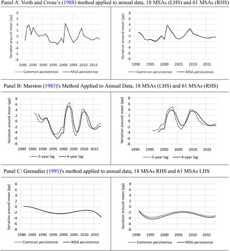
Both the Marston and the Voith and Crone models produce cycles that are like those in the long run ECM but the inversion of those in the short run ECM. In contrast, the estimates of time variation from the Grenadier model, shown in panel (C), based on a fourth order polynomial, are plausible in terms of smoothness and the ranges, of around 4% for the annual models and 2% for the quarterly models. However, the time pattern is different from that of the other two models. The secular trends are very gently downwards in all three models for the longer period, and very gently upwards for all models for the shorter period – the opposite of the ECM analysis.

Summary

Overall, these results point to two clear conclusions: there is no consistent evidence of a trend in the NVR over time for the US office market; and there is no evidence of any step changes.

The results raise concerns about existing approaches to estimating a time-varying NVR. While most approaches produce sensible and consistent estimates of the cross-section MSA variation in the NVR, estimates of time variation range widely, are inconsistent across the models, and are often implausible.

The rolling window estimates from the ECM models are sensitive to small changes in the constant and in the vacancy rate coefficient, both of which typically have very small magnitude. This is also a more general problem. The estimates derived from including time fixed effects in the ECM panel models seem, predominantly, to be picking up common national factors that are not included in the models. Both the Marston and the Voith and Crone models produce cycles that are the inversion of those in the short run ECM. Meanwhile, those models that impose a specific pattern of time variation lead to implausible means and/or standard deviations for the cross-section MSA estimates of the NVR.

Conclusion and Discussion

The natural vacancy rate is a key element to understanding the dynamics of real estate space markets, with market adjustments driven, inter alia, by deviations in the vacancy rate from its natural level. The concept of a natural vacancy rate (NVR) is similar to that of the natural rate of unemployment (NRU), but most empirical research has assumed that the NVR was constant despite the fact that factors thought to influence NVR, such as tenant mobility, search costs, holding costs and expectations about future demand, could vary over time. For instance, there were significant changes to tax laws in the 1980s that will have affected holding costs over time, while patterns of demand and characteristics of the stock will have changed over the long-term, although the net effect on NVR is uncertain.

We examined whether and how the NVR varies over time, adopting a range of approaches to estimate this variation, including extracting estimates from rental adjustment models and estimating persistence models. We analyzed the US office market, using both national time-series data and panel data for individual MSA markets. First, as a test of the models, we assumed a constant NVR and examined the cross-section MSA variation. Most approaches produced sensible and consistent estimates of the cross-section variation and these estimates correlate highly with the actual time series averages for the MSAs.

Next, we estimated temporal variation, but our results were much less convincing, with only rolling window estimates, which involve smoothing, producing generally plausible results. The cross-section variations in the NVR are affected by factors that have some, but not great, cross-section variation, and even less temporal variation over several decades. Our expectation was that, if the NVR varied over time, the variation would be gradual, in response to gradual shifts in structural factors affecting how space markets operate. Instead, although the secular trends were always very small, many estimates suggested that the NVR was both volatile and cyclical.

There are other factors that affect temporal variation in rent and rental adjustment, but not cross-section variation, because they are national variables, such as trends in the production and consumption of services, technology that affects space use, tax rates and depreciation policy. We are unable to include these explicitly within models that use time fixed effects, but it may be that their impact on rents swamps the estimates of time variation in the NVR. We conclude that many of our results reflect the inability of time dummies to isolate movements in the NVR from other factors driving real estate space markets.

Overall, the results are helpful in confirming the appropriateness of these modeling approaches in capturing the cross-section variation in the NVR. However, we have also established that serious issues arise when these approaches are used to model temporal variation in the NVR.

What implications does our research have for the modeling of real estate space markets? It is possible that the assumption of a constant NVR may be a practical and acceptable solution, particularly for shorter periods, but the behavior of the NVR over longer periods requires the exploration of different techniques used in labor economics, such as a variety of filter methods. However, the lack of a definitive result in the NRU/NAIRU literature suggests that there is no easy and obvious solution to the estimation of a natural rate, whether of unemployment or vacancy.

Acknowledgment

We thank CBRE Econometric Advisors for provision of most of the data used for this study.

Notes

1 Englund et al. (2008) and Hendershott et al. (2010) analyse, respectively, the Stockholm and London markets, where they estimated NVRs of around 7%. We are unable to model this effect satisfactorily, probably because the vacancy rate values of around 15% in our data are never low enough to generate the asymmetry.

2 Analogous to Taylor (1979), Englund et al. (2008) argued that “space occupancy, which depends on historical rents, often differs from demand at current rent” and that this “creates ‘hidden vacancies’ that can be positive or negative, vacancies that will develop in the future if market rent and the space demand driver are unchanged” (p. 81).

3 Nachane (2018) shows that, starting from a version of the Phillips Curve given by:

p = E(p) -a(u – NRU) + v

where p is inflation, E(p) is expected inflation, u is the rate of unemployment, NRU is the natural rate of unemployment, a is a constant and v is a supply shock, then NAIRU = NRU + (v/a).

4 In the original Phillips (1958) paper, the equation is w + a = bu^c, where a, b and c are constants. The equation is estimated as log (w + a) = log b + c log u.

5 For ease of expression, we use βs throughout although, clearly, these are not the same in every equation.

6 In fact, he is talking about the NAIRU; we use the term NRU for simplicity. He models it using, alternatively, the Phillips Curve and the Beveridge Curve (the relationship between unemployment and labor vacancies). He points to the large confidence intervals using the former and the easier and more robust approach using the latter.

7 More commonly, the real rate of rental increase has been modeled.

8 They examined 15 cities separately and a panel of 17 cities, with nominal rental change explained by the vacancy rate, or its lag, and lagged operating expenses. They derived estimates of the NVR that varied across cities but were constant in time, and they sought to explain the cross-sectional variation with several variables.

9 Englund et al. (2008) note that any change in the discount factor is likely to be partly capitalized into land prices, changing replacement cost (p. 93). Thus, the impact on equilibrium rent would be unknown (with full capitalization, there would be no impact).

10 He considered “the size of the minority population, and the level of housing market discrimination (how many landlords will forgo perspective tenants on the basis of race or color, etc.)” and concludes “that demographic variables like household mobility and minority population size also play a role in driving a change in the NVR.” He suggested that “Hendershott and Haurin (1988) provide a similar argument.”

11 Marston (1985) and Grenadier (1995) both include the time-varying component as part of the natural vacancy rate, while Voith and Crone (1988) include it in the error specification. The latter makes the algebra and the estimation easier but makes more difficult the interpretation of the role of the time-varying component in the natural vacancy rate. While Marston (1985) and Voith and Crone (1988) use time dummies, Grenadier (1995) uses a fourth order polynomial of t to reduce the number of parameters to be estimated.

12 Local CPI deflators are arguably more appropriate, but their availability is restricted to the largest urban areas and satellites of larger ones (37 of the 61 MSAs). Furthermore, the frequency of these series is not uniform. Quarterly inflation figures were available from the Bureau of Labor Statistics for some large MSAs, but only annual figures were available for others.

13 Table 1 indicates that there is similar variability in both the level of and change in vacancy rates between the two samples. However, the cross-sectional dispersion across the 18 MSAs is smaller and so the similar variation in the samples results from the inclusion of additional years.

14 Initially, we also estimated the nominal version of this equation with the lagged inflation rate as the proxy for expected inflation. The inflation variable was never significant, and, in the annual estimations, its coefficient was −0.066 for 1980–2018 and 1.987 for 1990–2018. The estimates of the constant NVR ranged from 11% to 19%. Accordingly, throughout our analyses, we have used real rent. While consistent with most of the real estate literature, it contrasts with the nominal approach used in most of the labor literature.

15 In this specification, rents are in log levels and the log difference is used as an approximation for the growth rate. Note that this differs from the Hendershott (1996) version in Equation (5)(5) $${rr}_t={\beta }_1\left(v_{t-1}-\mathit{NVR}\right)+{\beta }_2{(RR}_{t-1}-\mathit{EQRR})$$(5) which uses real rent and actual growth rates.

16 The error correction model (ECM) approach can also be undertaken in a single stage with the lagged values of the dependent and independent variables, rather than the residual, included in the difference equation. This is like Equation (3)(3) $$w_t={\beta }_0-\beta u_t+p_{(t-1)}-\lambda \left(W_{\left(t-1\right)}-P_{\left(t-1\right)}-Q_{\left(t-1\right)}\right)$$(3) from labor economics. It imposes less structure on the difference equation. However, in this version of the specification, the estimated constant now includes the constant from the long run model, so it is not possible to produce an estimate of the NVR.

17 There is evidence of autoregressive conditional heteroscedasticity (ARCH) for several of the estimations, particularly with quarterly data. Therefore, we used heteroscedastic and autocorrelation corrected (HAC) Newey and West (1987) standard errors to correct for potential autocorrelation and heteroscedasticity in the residuals.

18 We chose 10 years to minimize the impact of cycles and to produce an element of stability in the estimations. We also tried shorter and longer periods.

19 The model with the shock variables gives terrible results, with small coefficient values leading to huge jumps in the NVR from period to period, so we do not graph it.

20 Marston uses four and eight years; the Voith and Crone is Marston with a single year.

References

- Arnott, R., & Igarashi, M. (2000). Rent control, mismatch costs and search efficiency. Regional Science and Urban Economics, 30(3), 249–288. https://doi.org/https://doi.org/10.1016/S0166-0462(00)00033-8
- Ball, L., & Mankiw, N. G. (2002). The NAIRU in theory and practice. Journal of Economic Perspectives, 16(4), 115–136. https://doi.org/https://doi.org/10.1257/089533002320951000
- Barnichon, R., & Matthes, C. (2017). The natural rate of unemployment over the past 100 years. Federal Reserve Bank of San Francisco Economic Letter 2017–2023.
- Blanchard, O., & Katz, L. F. (1997). What we know and do not know about the natural rate of unemployment. Journal of Economic Perspectives, 11(1), 51–72. https://doi.org/https://doi.org/10.1257/jep.11.1.51
- Blank, D. M., & Winnick, L. (1953). The structure of the housing market. The Quarterly Journal of Economics, 67(2), 181–208. https://doi.org/https://doi.org/10.2307/1885333
- Brauer, D. (2007). The natural rate of unemployment (CBO Working Paper 2007-06). Congressional Budget Office.
- Claar, V. V. (2006). Is the NAIRU more useful in forecasting inflation than the natural rate of unemployment? Applied Economics, 38(18), 2179–2189. https://doi.org/https://doi.org/10.1080/00036840600701061
- Daly, M. C., Hobijin, B., Sahin, A., & Valletta, R. G. (2012). A search and matching approach to labor markets: Did the natural rate of unemployment rise? Journal of Economic Perspectives, 26(3), 3–26. https://doi.org/https://doi.org/10.1257/jep.26.3.3
- Dickens, W. T. (2009). A new method for estimating time variation in the NAIRU. In J. Fuhrer, Y. K. Kodrzycki, J. Sneddon Little, & G. P. Olivei (Eds.), Understanding inflation and the implications for monetary policy: A Phillips curve retrospective (pp. 207–230). MIT Press.
- Englund, P., Gunnelin, A., Hendershott, P. H., & Soderberg, B. (2008). Adjustment in property space markets: Taking long-term leases and transaction costs seriously. Real Estate Economics, 36(1), 81–109. https://doi.org/https://doi.org/10.1111/j.1540-6229.2008.00208.x
- Friedman, M. (1968). The role of monetary policy. American Economic Review, 58(1), 1–17.
- Gabriel, S. A., & Nothaft, F. E. (1988). Rental housing markets and the natural vacancy rate. Real Estate Economics, 16(4), 419–429. https://doi.org/https://doi.org/10.1111/1540-6229.00465
- Gabriel, S. A., & Nothaft, F. E. (2001). Rental housing markets, the incidence and duration of vacancy, and the natural vacancy rate. Journal of Urban Economics, 49(1), 121–149. https://doi.org/https://doi.org/10.1006/juec.2000.2187
- Gordon, R. J. (1997). The time-varying NAIRU and its implications for economic policy. Journal of Economic Perspectives, 11(1), 11–32. https://doi.org/https://doi.org/10.1257/jep.11.1.11
- Grenadier, S. R. (1995). Local and national determinants of office vacancies. Journal of Urban Economics, 37(1), 57–71. https://doi.org/https://doi.org/10.1006/juec.1995.1004
- Hall, R. E. (1979). A theory of the natural unemployment rate and the duration of employment. Journal of Monetary Economics, 5(2), 153–169. https://doi.org/https://doi.org/10.1016/0304-3932(79)90001-1
- Hendershott, P. H. (1996). Rental adjustment and valuation in overbuilt markets: Evidence from the Sydney Office Market. Journal of Urban Economics, 39(1), 51–67. https://doi.org/https://doi.org/10.1006/juec.1996.0003
- Hendershott, P. H., & Haurin, D. R. (1988). Adjustments in the real estate market. Real Estate Economics, 16(4), 343–353. https://doi.org/https://doi.org/10.1111/1540-6229.00459
- Hendershott, P. H., Jennen, M., & MacGregor, B. D. (2013). Modelling space market dynamics: An illustration using panel data for US retail. The Journal of Real Estate Finance and Economics, 47(4), 659–687. https://doi.org/https://doi.org/10.1007/s11146-013-9426-z
- Hendershott, P. H., & Kane, E. J. (1992). Causes and consequences of the 1980s commercial construction boom. Journal of Applied Corporate Finance, 5(1), 61–70. https://doi.org/https://doi.org/10.1111/j.1745-6622.1992.tb00482.x
- Hendershott, P. H., Lizieri, C. M., & MacGregor, B. D. (2010). Asymmetric adjustment in the City of London Office Market. The Journal of Real Estate Finance and Economics, 41(1), 80–101. https://doi.org/https://doi.org/10.1007/s11146-009-9199-6
- Hendershott, P. H., MacGregor, B. D., & Tse, R. Y. C. (2002a). Estimation of the rental adjustment process. Real Estate Economics, 30(2), 165–183. https://doi.org/https://doi.org/10.1111/1540-6229.00036
- Hendershott, P. H., MacGregor, B. D., & White, M. (2002b). Explaining real commercial rents using an error correction model with panel data. The Journal of Real Estate Finance and Economics, 24(1/2), 59–88. https://doi.org/https://doi.org/10.1023/A:1013930304732
- Marston, S. (1985). Two views of the geographic distribution of unemployment. The Quarterly Journal of Economics, 100(1), 57–79. https://doi.org/https://doi.org/10.2307/1885735
- Miceli, T. J., & Sirmans, C. F. (2013). Efficiency rents: A new theory of the natural vacancy rate for rental housing. Journal of Housing Economics, 22(1), 20–24. https://doi.org/https://doi.org/10.1016/j.jhe.2013.01.002
- Modigliani, F., & Papademos, L. (1975). Targets for monetary policy in the coming year. Brookings Papers on Economic Activity, 1975(1), 141–165. https://doi.org/https://doi.org/10.2307/2534063
- Nachane, D. M. (2018). Critique of the new consensus macroeconomics and implications for India. Springer.
- Newey, W. K., & West, K. D. (1987). A simple, positive semi-definite, heteroskedasticity and autocorrelation consistent covariance matrix. Econometrica, 55(3), 703–708. [Database] https://doi.org/https://doi.org/10.2307/1913610
- Perry, G. L. (1970). Changing labor markets and inflation. Brookings Papers on Economic Activity, 1970(3), 411–448. https://doi.org/https://doi.org/10.2307/2534139
- Phelps, E. S. (1967). Phillips curves, expectations of inflation and optimal unemployment over time. Economica, 34(135), 254–281. https://doi.org/https://doi.org/10.2307/2552025
- Phelps, E. S. (1968). Money-wage dynamics and labor-market equilibrium. Journal of Political Economy, 76(4), 678–711. https://doi.org/https://doi.org/10.1086/259438
- Phillips, A. W. (1958). The relation between unemployment and the rate of change of money wage rates in the United Kingdom, 1861-1957. Economica, 25(100), 283–299. https://doi.org/https://doi.org/10.1111/j.1468-0335.1958.tb00003.x
- Pollakowski, H. O., Wachter, S. M., & Lynford, L. (1992). Did office market size matter in the 1980s? A time-series cross-sectional analysis of metropolitan area office markets. Journal of the American Real Estate and Urban Economics Association, 20(1), 303–324.
- Posta, V. (2008). The NAIRU and the natural rate of unemployment – A theoretical view (Research Study No. 1/2008). The Ministry of Finance of the Czech Republic.
- Read, C. (1993). Tenants’ search and vacancies in rental housing markets. Regional Science and Urban Economics, 23(2), 171–183. https://doi.org/https://doi.org/10.1016/0166-0462(93)90002-V
- Rosen, K., & Smith, L. B. (1983). The price adjustment process for rental housing and the natural vacancy rate. American Economic Review, 73(4), 779–786.
- Samuelson, P. A., & Solow, R. M. (1960). Analytical aspects of anti-inflation policy. American Economic Review, 50(2), 177–194.
- Shilling, J. D., Sirmans, C. F., & Corgel, J. B. (1987). Price adjustment process for rental office space. Journal of Urban Economics, 22(1), 90–100. https://doi.org/https://doi.org/10.1016/0094-1190(87)90051-9
- Sivitanides, P. (1997). The rent adjustment process and the structural vacancy rate in the commercial real estate market. Journal of Real Estate Research, 13(2), 195–209. https://doi.org/https://doi.org/10.1080/10835547.1997.12090875
- Staiger, D., Stock, J. H., & Watson, M. W. (1997). How precise are estimates of the natural rate of unemployment? In C. D. Romer & D. H. Romer (Eds.), Reducing inflation: Motivation and strategy (pp. 195–246). University of Chicago Press.
- Taylor, J. B. (1979). Staggered wage setting in a macro model. American Economic Review Papers and Proceedings, 69(2), 108–113.
- Thirlwall, A. P. (1983). What are estimates of the natural rate of unemployment measuring? Oxford Bulletin of Economics and Statistics, 45(2), 173–179. https://doi.org/https://doi.org/10.1111/j.1468-0084.1983.mp45002002.x
- Tobin, J. (1997). Supply constraints on employment and output: NAIRU versus natural rate. Cowles Foundation Discussion Papers 1150, Cowles Foundation for Research in Economics, Yale University.
- Vandell, K. (2003). Tax structure and natural vacancy rates in the commercial real estate market. Real Estate Economics, 31(2), 245–267. https://doi.org/https://doi.org/10.1111/1540-6229.00065
- Voith, R., & Crone, T. (1988). National vacancy rates and the persistence of shocks in U.S. office markets. Real Estate Economics, 16(4), 437–458. https://doi.org/https://doi.org/10.1111/1540-6229.00467
- Wheaton, W. C., & Torto, R. G. (1988). Vacancy rates and the future of office rents. Real Estate Economics, 16(4), 430–436. https://doi.org/https://doi.org/10.1111/1540-6229.00466
- Wheaton, W. C., Torto, R. G., & Southard, J. A. (1997). The CB Commercial/Torto Wheaton database. Journal of Real Estate Literature, 5(1), 59–66. https://doi.org/https://doi.org/10.1080/10835547.1997.12090059
- Zabel, J. (2016). A dynamic model of the housing market: The role of vacancies. The Journal of Real Estate Finance and Economics, 53(3), 368–391. https://doi.org/https://doi.org/10.1007/s11146-014-9466-z
- Zhou, J. (2008). Estimating natural vacancy rates with unknown break points for the Chicago rental housing market. Journal of Housing Research, 17(1), 61–74. https://doi.org/https://doi.org/10.1080/10835547.2008.12091987