A swingogram representation for tracking micro-rhythmic variation in jazz performances

Abstract

A typical micro-rhythmic trait of jazz performances is their ‘swing feel.’ According to several studies, uneven eighth notes contribute decisively to this perceived quality. In this paper we analyze the swing ratio (beat-upbeat ratio) implied by the drummer on the ride cymbal. Extending previous work, we propose a new method for semi-automatic swing ratio estimation based on pattern recognition in onset sequences. As a main contribution, we introduce a novel time-swing ratio representation called swingogram, which locally captures information related to the swing ratio over time. Based on this representation, we propose to track the most plausible trajectory of the swing ratio of the ride cymbal pattern over time via dynamic programming. We show how this kind of visualization leads to interesting insights into the peculiarities of jazz musicians improvising together.

Keywords:

• Music information retrieval
• rhythmic features
• microrythm
• jazz music
• swing ratio

1. Introduction

Rhythm and meter constitute essential building blocks of music and are perhaps some of the most accessible aspects for non-expert listeners. The metrical framework that is realized through regular rhythmic structure often induces a motor response of the listener to the music, e.g. tapping one’s feet or nodding one’s head. Additionally, rhythmic and micro-rhythmic structures contribute to a specific character of the music that humans describe as ‘swinging,’ ‘driving’ or ‘groovy’ (Davies, Madison, Silva, & Gouyon, 2013). In this work, we seek to automatically analyze micro-rhythmic variations in the course of recorded jazz solos.

While jazz drummers often emphasize accents of the compositions during the opening and closing thematic sections of a jazz recording, they usually keep time during the solo sections using the ride cymbal (RC) and hi-hat (HH). Thereby, the RC is struck on every beat (i.e. quarter note) while the HH pedal is played on every second beat, i.e. beats two and four in a 4 / 4 bar. Instead of playing the RC steadily, intricate variations and additional offbeat strokes are usually intertwined on the RC as well as on other drum parts, especially in styles with so-called swing feel (Berliner, 1994).

Figure 1. Illustration of prototypical RC patterns as drum notation (top), time-domain signal (mid), and LLACF (bottom). Besides the black quarter notes, the relevant eighth notes are coded by light green (onbeat), and hatched, light red (offbeat). (a) Swing ratio of corresponding to straight eighth notes, i.e. onbeat and offbeat having the same duration. (b) Swing ratio of corresponding to the idealized tied-triplet notation. (c) Swing ratio , where the onbeat can be notated as a dotted eighth note and the offbeat as a sixteenth note.

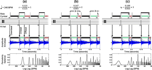
The most common, prototypical RC pattern is depicted in Figure 1. In addition to the drum notation in the top row, a corresponding time-domain signal at 240 BPM with overlaid amplitude envelope (thin black curve) as well as an onset-related novelty function (bold black curve) are shown in the middle row. In this figure, the RC onsets, as well as their inter-onset-intervals (IOIs), are color-coded as follows. The sequence starts with a downbeat quarter note (black), followed by an onbeat eighth note (light green), and an offbeat eighth note (hatched, light red). This three-note pattern is then repeated. We will re-use these color-codes throughout the paper, with black indicating any note object that is not considered for measuring swing ratios.

Within jazz performances, the musicians deliberately introduce micro-rhythmic variations to convey the typical character of the music. Jazz drummers often play swinging eighth notes, i.e. they modify the beat subdivision and phrasing of the eighth notes in the RC pattern. Swinging eighth notes are typically performed in different ratios, on a continuous scale ranging from straight eighths (1 : 1), over tied-triplet eighths (2 : 1), to dotted eighths (3 : 1), and occasionally even more extreme ratios. For example, in Figure 1(a)–(c), the color-coded rectangles depict how the onbeat IOI (the time interval between onbeat and subsequent offbeat) grows with increasing swing ratio. In contrast, the offbeat IOI (the time interval between offbeat and next beat) shrinks. In Figure 1(a), onbeats and offbeats have equal IOIs, corresponding to straight eighths as typically specified in drum notation. In Figure 1(b), the swinging eighth notes are notated as tied-triplets. In Figure 1(c), the onbeat IOI equals a dotted eighth, resulting in an offbeat IOI corresponding to a sixteenth note.

According to many authors, the swing ratio generally depends on the tempo (cf. Section 2.1). Few works specifically examine the RC pattern (Honing & de Haas, 2008) and its interaction with the soloist’s microtiming (Friberg & Sundström, 2002). In order to accumulate more data on micro-rhythm in jazz recordings, we introduced a semi-automatic method for swing-ratio estimation from RC patterns (Dittmar, Pfleiderer, & Müller, 2015). As a main contribution of the current study, we propose an extension to our previous method by introducing a novel time-swing ratio representation that captures the time-varying characteristics of the swing ratio. We apply this method to provide intuitive visualizations of micro-rhythmic variations throughout a jazz performance. We demonstrate the potential of our new method by introducing a tool that can be used by musicologists for analyzing RC swing ratios in relation to tempo, jazz style, and personal preferences of drummers within the history of jazz.

The remainder of this paper is structured as follows. In Section 2, we discuss related work dealing with swing analysis and extraction of rhythmic features in general. In Section 3, we introduce our novel swingogram representation for visualizing swing-ratio characteristics over time. In particular, we explain the most important swingogram properties and provide details on our proposed extraction strategy. In Section 4, we evaluate the robustness of our approach for swing-ratio estimation from jazz solo recordings. Then, in Section 5, we apply the swingogram method to point out some preliminary observations about the micro-rhythmic interplay of soloists and drummers in interesting jazz solo recordings. Finally, we conclude and outline important directions for future work in Section 6.

2. Related work

In the following two sections, we provide a brief overview of related work that is relevant for our study. Since our research is positioned at the intersection of jazz research and music information retrieval (MIR), we try to cover both aspects. We first discuss some papers with systematic studies on swing ratio in jazz music and then briefly summarize MIR methods that have been proposed for rhythm pattern analysis.

2.1. Jazz microtiming analysis

An early attempt to analyze swing ratios in jazz solos is described by Kerschbaumer (1978). The author relies on visual inspection of spectrograms but does not report quantitative results. According to Reinholdsson (1987), swing ratios in the analyzed jazz solos range from 1.48 to 1.82. Rose (1989) reports an average swing ratio of 2.38 measured from amplitude envelopes of the RC. Ellis (1991) measured an average swing ratio of 1.75 using a MIDI wind controller played by saxophonists. Parsons and Cholakis (1995) focus on the RC and report swing ratios between 1.0 and 3.3 without detailing the measurement method. Collier and Collier (2002) measured an average swing ratio of 1.6 by inspecting amplitude envelopes of soloists recordings. Busse (2002) measured an average swing ratio of 2.45 in the performances of pianists playing a MIDI piano. A more comprehensive overview on scientific studies about swing is given by Pfleiderer (2006) and Wesolowski (2012). In the following paragraphs, we focus on publications that are closely related to our current study.

Fundamental to our work is the study by Friberg and Sundström (2002), who investigated the swing ratio between the onbeat and offbeat in RC patterns by annotating spectrogram excerpts. Their results indicate a linear, negative correlation between the tempo and the swing ratio, which seems to be valid across various drummers. At comparatively slow tempi, the swing ratio reaches up to 3.5, as opposed to fast tempi where it decreases to 1.0. Furthermore, the authors argue that the minimum duration of the offbeat in RC patterns is around 100 ms, suggesting that there exists an upper limit to the swing ratio achievable at high tempi. In addition, they provide some evidence that the soloists usually play behind the beat of the rhythm section, and perform at a lower swing ratio than the drummer in order to synchronize their offbeats with those of the RC.

Benadon (2006) measured comparably low swing ratios up to 1.7 from amplitude envelopes. Additionally, Benadon (2006) states that some specific melodic and harmonic features as well as phrase structure and rhythmic peculiarities are elucidated by micro-rhythmic characteristics. Among others, he found a higher swing ratio at phrase endings. Benadon (2006) hypothesizes that at these endings the soloist tries to better synchronize to the drummer’s RC patterns.

Honing and de Haas (2008) conducted experiments with professional jazz drummers performing on a MIDI drum kit. Besides further evidence for the tempo dependency of swing ratios, their results show that jazz drummers have very exact control over their timing. However, they do not conclude that the swing ratio is a linearly decreasing function of tempo. Similarly, Marchand and Peeters (2015) report that the swing ratio does not exhibit a linear relationship at tempi lower than 130 BPM and instead shows a preference for the tied-triplet swing ratio around 2.0. Their results are based on manual annotation of downbeat, beat and eighth-note positions for all recordings contained in the GTZAN corpus (Sturm, 2012). However, their study does not specifically focus on jazz performances so the results have to be interpreted carefully.

Davies et al. (2013) studied the perception of micro-rhythmic variations. Synthesized rhythm patterns with systematic timing deviations were presented to different groups of listeners who were asked to rate naturalness and liking. Interestingly, only jazz patterns received high ratings when systematic microtiming was introduced by means of swinging eighth notes.

The majority of the studies mentioned above have in common a two-stage procedure. In the first stage, a manual annotation of the recordings under analysis is performed, which is a labor-intensive process. In the second stage, an interpretation of the annotated data is devised and, occasionally, compared with listeners responses. When considering large-scale studies, it is important to automate the first step as much as possible. Some researchers have tried to solve this issue by equipping jazz musicians with MIDI instruments (Ellis, 1991; Busse, 2002; Honing & de Haas, 2008) and asking them to play under more or less artificial conditions.

In our work, we aim to provide tools that alleviate the annotation process in a semi-automatic manner, thus generating a much larger data sample as was available so far. Furthermore, to better handle large amounts of data, we provide intuitive visualizations via our novel swingogram that immediately exhibits peculiarities of swing-ratio variations within jazz recordings. In Section 5, we will demonstrate with concrete examples how studies of micro-rhythm may benefit from the new method.

2.2. Rhythmic mid-level features

In MIR, a central paradigm is to convert digitized music recordings into suitable feature representations enabling pattern recognition and retrieval in extensive music corpora. Typically, the first step is to extract ‘low-level features’ which can be computed directly from the audio waveform or equivalent time-frequency representations, such as the short-time Fourier transform (STFT). Besides simple amplitude envelopes (Dixon, Gouyon, & Widmer, 2004), many different features have been proposed that emphasize transient events in the signal. For example, spectral flux (Dixon, 2006) and novelty curves (Müller, 2015) are commonly used in rhythm analysis. More recently, several authors advocate to use learned feature representations that are optimized for beat or downbeat tracking by means of training deep neural networks (Böck, Arzt, Krebs, & Schedl, 2012; Eyben, Böck, Schuller, & Graves, 2010).

Avoiding the explicit detection of note onset events, time-series of such low-level features can be directly analyzed with regard to re-occurring or quasi-periodic peak patterns. In general, two different families of methods are established for measuring periodicities. Techniques based on the autocorrelation function (ACF) (Kurth, 2013; Marchand & Peeters, 2015) allow to detect periodic self-similarities by comparing a time-series with time-shifted copies of itself. Alternatively, Fourier-based methods such as the beat spectrum (Foote & Uchihashi, 2001; Peeters, 2005) compare a time-series with sinusoidal templates representing specific frequencies. Both methods reveal periodicities and local self-similarities, which in turn are the most important cues for rhythmic pattern analysis. For example, the beat spectrum exhibits peaks at frequencies corresponding to the strongest periodicity and its integer multiples. In contrast, the ACF exhibits peaks at integer factors of the strongest periodicities. In an analogy to pitch analysis, these series of peaks are commonly called harmonics, respectively subharmonics. Since it is often difficult to determine which peak corresponds to the rhythmic level of interest (e.g. the beat), one uses the notion of octave ambiguity. To avoid such uncertainties, Kurth et al. (2006) proposed a cyclic post-processing to accumulate rhythmic patterns across all octaves.

Both the ACF and the beat spectrum are often referred to as ‘mid-level features’, expressing that they reside on a higher semantic level than the underlying low-level time-series. Ideally, mid-level representations should capture relevant characteristics and remain invariant to aspects irrelevant for the given analysis task. For example, certain rhythmic patterns may be perceived as similar by human listeners even when they are played in a different tempo. Unfortunately, both beat spectrum and ACF are clearly not invariant to tempo differences. As an example, increasing the tempo leads to a compression of the lag-axis underlying the ACF. To counter these problems, several authors proposed conceptually similar post-processing techniques.

Both Dixon et al. (2004) and Peeters (2005) proposed to warp mid-level features to a common axis normalized to the given bar length. Once converted to this tempo-normalized representation, rhythmic patterns can be compared by simple distance measures, or further rhythmic features can be derived. For example, Marchand and Peeters (2015) employed a tempo-normalized peak-fitting model of the ACF for swing ratio estimation.

In order to avoid tempo-informed normalization, Holzapfel and Stylianou (2009), Holzapfel and Stylianou (2011) proposed to apply the scale transform to ACF-based mid-level features. In theory, the scale transform magnitude of the same rhythmic pattern played in different tempi should be similar up to a constant scaling factor. In practice, the scale transform leads to a new feature representation that is less susceptible to tempo differences. Marchand and Peeters (2014) applied the scale transform to modulation spectra, yielding tempo-independent features for the classification of ballroom dances. Similarly, Prockup, Ehmann, Gouyon, Schmidt, and Kim (2015) used the scale transform to derive further descriptors used for the classification of ballroom styles and microtiming characteristics such as swing and shuffle.

The log-lag autocorrelation (LLACF), one of the main ingredients for our method (see Section 3.3.2), was introduced by Gruhne and Dittmar (2009). Around the same time, Jensen, Christensen, and Jensen (2009) proposed a similar, tempo-insensitive representation for ballroom dance classification. In essence, both techniques are based on warping the linearly-spaced lag-axis of the ACF to a logarithmic spacing. The rationale is convert compression (faster tempo) or stretching (slower tempo) of the lag-axis into constant offsets along the log-lag axis. Völkel, Abeßer, Dittmar, and Großmann (2010) reported that the LLACF is favorable over the scale transform for classification of Latin American rhythm patterns. Eppler, Männchen, Abeßer, Weiß, and Frieler (2014) used peak ratios in the LLACF as features for detecting the presence of swing. In our own previous work (Dittmar et al., 2015), we proposed to employ LLACF-based pattern matching to estimate the swing ratio of jazz excerpts. In the following section, the main concepts of our previous paper will be recapitulated for the sake of clarity.

3. Swingogram representation

In order to semi-automatically track the temporal variation of the drummer’s swing ratio in jazz recordings, we introduce suitable features that capture relevant properties while suppressing irrelevant or confounding information. Given a jazz recording, our core idea is to first extract sequences of LLACF vectors (Dittmar et al., 2015) in a segment-wise fashion. These sequences are then converted into a two-dimensional representation that indicates the likelihood of certain swing ratios for each time position. As we will show, our novel representation is, to a certain degree, invariant to tempo changes. Moreover, it can be explicitly interpreted like a spectrogram, with a swing-ratio axis instead of a frequency axis. In reference to the music genre of this study and acknowledging the history of well-known signal representations, such as spectrograms, scalograms (Rioul & Vetterli, 1991), chromagrams (Bartsch & Wakefield, 2005), rhythmograms (Jensen, 2007), or tempograms (Grosche & Müller, 2011a), we call our novel mid-level representation swingogram.

3.1. Illustrative example of the Swingogram

First, let us take a look at the instructive example in Figure 2 to illustrate the most important properties of the swingogram. We show different signal representations of a synthetic music example that contains 100 repetitions of the RC pattern from Figure 1(b) (tied-triplet feel). Throughout this signal, we steadily increase the tempo with every four beats, yielding a tempo sweep between 146 BPM and 328 BPM. We aim to show that the swing-related properties of the synthetic music signal are contained in each of the three representations, but are most readable in the swingogram. We recommend to take a look at a larger version of Figure 2 on our accompanying webpage¹ where the music signal can be auditioned in synchronicity with a cursor showing the current playback position inside each of the signal representations.

Figure 2. Different representations of an RC pattern played with increasing tempo. (a) The STFT-based tempogram as described by Grosche and Müller (2011a). (b) The segment-wise sequence of LLACF patterns (see Section 3.3.2). (c) The corresponding swingogram representation.

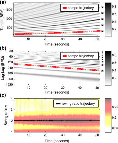
In Figure 2(a), we show a well-known time-tempo representation called tempogram (Grosche & Müller, 2011a). The tempogram is obtained by segment-wise processing of a novelty curve (see Section 3.3.2) with respect to local periodic patterns via STFT. The darker shades of gray encode salient periodicities, while the red curve with white dashes shows the underlying tempo trajectory used in the synthesized signal. To the right side of the tempogram, we mark the position of all integer multiples of the final tempo by black crosses. The second tempo harmonic (third black cross from the bottom up) exhibits the highest peak since it best explains the virtual subdivision of the beat that is inherent to the tied-triplet feel. Note that additional, weaker peaks appear in between the tempo multiples (visible as ridges of lighter shade of gray). These are explained by the periodicity of half the bar-length, i.e. when the RC pattern repeats. Since the tempo changes over time, the tempogram exhibits the same pattern stretched in vertical direction with increasing tempo.

Similarly, in Figure 2(b), we show the sequence of segment-wise LLACF vectors (Dittmar et al., 2015). For the moment, it is important to note that with LLACFs, the stretching observed in Figure 2(a) transforms into a linear shift along the vertical axis in Figure 2(b). This is underlined by the fact that the tempo trajectory now exhibits a linear slope. Furthermore, note that the vertical axis is reversed w.r.t. Figure 2(a) for the sake of consistency with prior work. We again place black crosses to the right of the LLACF sequence, this time marking the position of the final tempo and its integer factors (tempo subharmonics). Weaker peaks between these tempo values are a result of the characteristic swing pattern. We will discuss the peculiarities of the LLACF and the interpretation of its log-lag axis in more detail in Section 3.3.2.

Finally, in Figure 2(c), we show the swingogram extracted from the LLACF representation of Figure 2(b). To emphasize that the swingogram is in a different domain than the previous representations, we encode the values of its elements by a different colormap. Light yellow areas correspond to low likelihood for a certain swing ratio, whereas dark red areas correspond to high values. The black line shows the swing-ratio trajectory that can be tracked via dynamic programming (DP) (see Section 3.4). As expected, the trajectory essentially follows the value 2.0 (tied-triplet feel) over the complete duration of our example signal. This clearly shows that the swingogram, as desired, is largely invariant to the tempo changes. In our example, the tempo sweep covers 182 BPM starting with 146 BPM and ending with 328 BPM. Still, the underlying swing ratio can be estimated quite accurately.

3.2. Swing ratio

Before we move on with the details of the proposed extraction method, we now give a proper definition of the swing ratio as used in this paper. Let be the onbeat IOI and be the offbeat IOI, i.e. the physical time intervals in the RC pattern as shown in Figure 1. The sum of both IOIs equals the beat periodicity denoted by . Then, the swing ratio is defined by(1)

In the case that the swing ratio and beat periodicity are known, one can compute the onbeat and offbeat IOIs via the formulas and .

Following earlier works, we assume that in jazz recordings, reasonable swing ratios can take any value in the range between and . Formally, we express this by introducing the set of possible swing ratios , with . In practice, we sample a number of discrete prototype swing ratios from [1, 4], assuming that . This will be explained in more detail in Section 3.3.3.

3.3. Extraction procedure

Guided by Figure 3, we now give a brief overview of our proposed extraction procedure. We refer to the following subsections for details on the individual processing steps.

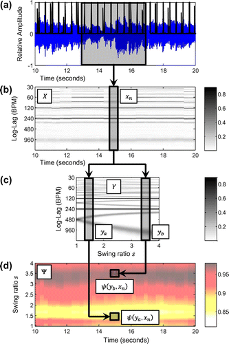
In short, we propose to first extract a novelty curve (see Section 3.3.1) from the music waveform (Figure 3(a)). Subsequently, segments of the novelty curve are converted into LLACF vectors (see Section 3.3.2). As indicated by the gray boxes in Figure 3(c), each LLACF vector is compared against LLACF prototype patterns (see Section 3.3.3) by means of a similarity measure (see Section 3.3.5). Finally, in Figure 3(d) the resulting similarity scores yield the elements of a swingogram matrix (see Section 3.3.4).

Figure 3. Overview of the proposed procedure for computing the swingogram. (a) Input waveform of a jazz music excerpt (in blue), overlayed with the onset-related novelty curve (black curve). (b) The sequence X of LLACFs extracted in a segment-wise fashion from the novelty curve. The salience of the periodicity peaks is encoded in the gray scale. (c) The set Y of LLACF prototype patterns. The salience of the periodicity peaks is encoded in the gray scale. Note that the horizontal axis refers to the range of considered swing ratios. (d) The resulting swingogram  after computing the similarity score as described in Section 3.3.4.

3.3.1. Novelty curve

In Figure 3(a), the waveform of a jazz music excerpt is shown in blue. In black, we overlay the corresponding novelty curve, i.e. a time-series that exhibits salient peaks at the temporal position of onset candidates (Grosche & Müller, 2011b). Given a music signal waveform, the first step for extracting the novelty curve is to convert the signal to an equivalent time-frequency representation using the STFT. Following our previous paper (Dittmar et al., 2015), the STFT uses a window size of approximately 46 ms and a hop size of approximately 6 ms. By applying logarithmic compression to the STFT magnitude and subsequently accumulating the positive spectral changes between consecutive frames, one obtains the novelty curve. Peak positions of this curve indicate note onset candidates, see also chapter 6 of the book (Müller, 2015) for details.

RC onsets typically lead to clearly visible transients (i.e. vertical spectral structures) in the upper frequency regions. Thus, we only consider spectral changes in a high-pass frequency band, at the same time attenuatingspurious peaks from other instruments. In our previous paper (Dittmar et al., 2015), we evaluated the suitability of this novelty curve for the detection of RC onsets in jazz excerpts. Testing against 834 RC onsets annotated by human experts, we received an F-measure of approximately 0.93 using a tolerance of ms around the true positions. However, especially with older jazz recordings, strongly attenuated high frequency content or crackling and other distortion might lead to severe degradation. Here, more sophisticated extraction strategies based on drum transcription techniques may be applied (Dittmar & Gärtner, 2014; Southall, Stables, & Hockman, 2016; Röbel, Pons, Liuni, & Lagrange, 2015; Vogl, Dorfer, & Knees, 2017; Wu & Lerch, 2015).

3.3.2. Log-lag autocorrelation function

As indicated by the gray box in Figure 3(a), we extract LLACF vectors from overlapping frames of the novelty curve. Throughout this paper, we use a frame size of approximately 4 s in conjunction with a hop size of 250 ms between consecutive frames. In essence, LLACF vectors capture the salience of localized periodic repetitions apparent in the novelty curve. For our task, the LLACF serves as a tempo-normalized mid-level representation for rhythmic patterns (Dittmar et al., 2015; Gruhne & Dittmar, 2009). To compute the LLACF vectors, we first apply the conventional autocorrelation function (ACF) of the novelty curve inside each frame. Afterward, we use linear interpolation to warp the ACF onto a log-lag axis. This new axis is defined in a way that it exhibits equal spacing between tempo octaves and has a reference tempo at a defined position.

Let us explain in more detail how we interpret the log-lag axis in BPM. In general, a lag value (in seconds) can be converted to a tempo value (in BPM) as(2)

The reciprocal relationship between tempo and lag turns into a negative relationship when applying the binary logarithm(3)

The rationale behind using the binary logarithm is to yield unit spacing between tempo octaves, i.e. tempo and twice the tempo . Formally, this can be expressed as(4)

for arbitrary tempo values . As a consequence, log-tempo and log-lag axis can be interpreted as two sides of the same coin. Once we warp either tempo or lag to binary logarithmic spacing, we can easily switch between both by applying a sign flip (and an offset). This explains why we give the log-lag axis in BPM but in reverse order to the usual orientation.

Figure 4. Schematic overview of the construction of reference patterns.

For the following extraction steps, let be an LLACF vector, with being the number of elements of the discrete log-lag axis. Furthermore, let , be a sequence of LLACF vectors , with . In this context, is the number of frames, each of which can be assigned a physical center point. Examples of such LLACF sequences are shown in Figures 2(b) and 3(b).

Complementary to the mathematical definition, let us take a look at the bottom row of Figure 1 to get an intuition about how the typical shape of an LLACF changes when fixing the tempo but varying the swing ratio. In Figure 1, a pronounced peak at 240 BPM can be seen which represents the periodicity of the beat IOI . Slightly higher peaks occur at integer factors of this periodicity, corresponding to the tempi BPM. Note that the sequence of onsets in our prototype RC pattern explains why these tempo subharmonics exhibit a stronger periodicity than the beat itself. As already stated in Section 1, the RC pattern repeats after a sequence of downbeat, onbeat, and offbeat, i.e. after two quarter notes. Thus, the highest self similarity of the RC pattern is obtained at half the bar-length. Similar phenomena often lead to octave ambiguity in rhythmic mid-level features as discussed in Section 2.2.

Regardless of these issues, it is important to note that the beat-related peaks remain fixed with increasing swing ratio, while the peaks corresponding to the eighth note IOIs at 480 BPM (and their subharmonics) split up in two peaks of lower salience which encode the characteristic relationship between the onbeat IOI and the offbeat IOI . For example, in the case of , the left-most peak resides at 960 BPM, which is exactly the periodicity of a sixteenth note at 240 BPM. In the following, we will refer to these characteristic local maxima as side-lobe peaks. We exploit their relative location as most important cue for estimating the underlying swing ratio.

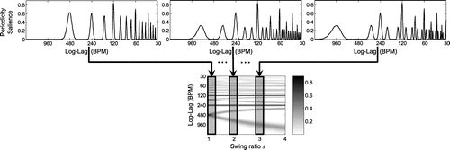
3.3.3. LLACF prototype patterns

As discussed earlier, our swingogram method reflects the likelihood of certain swing ratios being present in an observed LLACF vector . The estimation of this likelihood is based on pattern matching against LLACF prototype patterns with known swing ratios. These are obtained by sampling swing ratios for and creating ideal LLACF prototype patterns for each discrete swing ratio. In the following, we denote these patterns as . They are obtained by applying the processing steps described above to artificial novelty curves representing the RC pattern with a fixed reference tempo (we use 240 BPM throughout this work). In Figure 4, we illustrate this principle, revisiting the three example LLACFs from Figure 1 at swing ratios . As indicated by the gray boxes in the bottom part of Figure 4, the three prototype patterns are only a small subset of all prototype patterns.

In practice, we represent the set of prototype patterns by a matrix containing the prototype LLACFs as its columns. In the bottom of Figure 4 we depict the matrix , encoding salient peaks of the prototype LLACFs by darker shades of gray. It is important to note that, opposed to the matrix (see Section 3.3.2), the horizontal axis now encodes the swing ratio and not time. The above mentioned characteristic side-lobe peaks induced by the eighth notes are clearly visible as curved ridges diverging more and more from their initial position (at 480 BPM) with increasing swing ratio Note how the same behavior repeats for the multiples of the side-lobe peaks between the stronger peaks corresponding to the beat periodicity and its multiples (at BPM).

3.3.4. LLACF pattern matching

Returning to Figure 3(b), we now give an intuitive explanation of our approach to LLACF pattern matching. The slice marked with a dark gray box represents a single LLACF vector extracted from the temporal segment marked in gray in Figure 3(a). On closer inspection, one might recognize a side-lobe peak around 960 BPM. Recall that we encountered a similar side-lobe peak in the right-most panel in Figure 4. This indicates a high likelihood for a swing ratio at but the question remains how we can arrive at this analysis in an automated fashion.

Let us introduce the notion of a similarity function:(5)

Typically, is high if and are similar to each other, and otherwise is small. Evaluating the local similarity score for each pair and , we obtain the swingogram matrix defined by(6)

for (representing time) and (representing swing ratios).

A conceptual illustration for this procedure is provided by the arrows and boxes connecting Figure 3(b)–(d). They show how the element of is compared against two prototype patterns and (columns) of . More explicitly, the LLACF prototype pattern corresponds to , while the second prototype pattern corresponds to . By visual comparison of the pattern in with both and , we can see that the LLACF vector under analysis is more similar to the second LLACF prototype pattern. Thus, one obtains and the value is larger than as indicated by the color-coding Figure 3(d).

3.3.5. LLACF similarity measure

The notion of likelihood or similarity is of crucial importance in our proposed method. We did not discuss this issue at length before, but we already showed in Figure 2(b) that tempo deviations lead to shifts of the LLACF patterns along the vertical log-lag axis. These potential shifts need to be accounted for when comparing an LLACF vector to an LLACF prototype pattern . Therefore, we proposed to use the maximum value of the normalized cross-correlation as a similarity measure (Dittmar et al., 2015). The rationale was to impose invariance to slight tempo differences which might be present due to local deviations from the reference tempo. With slightly simplified notation, our previous similarity score can be expressed as:(7)

for , where the vector is suitably zero-padded. In other words, we only considered the maximum correlation when is shifted against .

In this paper, we introduce an alternative, more efficient method for comparing and . To this end, we transform and into equivalent representations by computing the complex-valued Discrete Fourier Transform (DFT) and taking the modulus (i.e. absolute value). The rationale is that the above-mentioned log-lag shifts result in phase offsets in the corresponding DFT coefficients. Discarding the phase information makes the similarity score robust against such effects. If we compare an LLACF vector with itself, we want to achieve a similarity score of , thus we normalize the DFT magnitude vectors by subtracting their arithmetic mean and dividing the results by their standard deviation. With regard to our notation introduced above, we call the resulting vectors and . This transformation has to be computed only once for the fixed LLACF prototype patterns . Finally, our similarity score simplifies to an inner product:(8)

Clearly, this is a much more streamlined and elegant procedure than the one proposed in our previous work (Dittmar et al., 2015).

3.4. Swing ratio tracking

In order to obtain a trajectory of the swing ratios in , one could go from left to right through each of the columns, each time picking the maximum element and looking up the corresponding swing ratio . However, this might not be robust against sudden jumps. In order to achieve smooth trajectories considering the temporal context, we propose to use Dynamic Programming (DP) as a standard technique to find an optimal path that maximizes the similarity score among all possible paths in . The general idea behind DP is to use an accumulated similarity matrix and store local maximum decisions to recursively find the score-maximizing path (Ellis, 2007; Müller, 2015). Furthermore, constraints can be added on the allowed local slope of the trajectory when going from one column to the next.

For our scenario, we make two assumptions for the application of DP. First, we presume that the drummer will change the swing ratio only gradually from frame to frame. Second, the LLACF prototype patterns encoded by are generated according to the continuously increasing scale of swing ratios. The typical outcome of a DP-based tracking is overlayed as a black path on top of swingogram  in Figure 2(c).

4. Evaluation

In this section, we evaluate the quality of swing-ratio estimates derived with our swingogram representation. First, in Section 4.1, we give an overview of the manually annotated jazz excerpts we use as ground truth data. Then, in Sections 4.2 and 4.3, we present the experimental results from two perspectives.

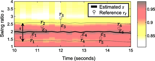
Figure 5. Deviation and tolerance that we employ for evaluating our proposed method.

4.1. Data set and annotations

To a large extent, our research is driven by the Jazzomat Research Project (Frieler, Zaddach, Abeßer, & Pfleiderer, 2013). The project aims to investigate the creative processes underlying jazz solo improvisations via computational methods. The overarching goal is to explore the cognitive and cultural foundations of jazz solo improvisation. As a basis for our work, we can use the jazz solo transcriptions and music recordings of the Weimar Jazz Database (WJD² ) that has been created within the Jazzomat project.

The WJD consists of 430 (as of February 2017) transcriptions of instrumental jazz solo recordings performed by a wide range of renowned jazz musicians. These recordings are characterized by a predominant, monophonic solo instrument (e.g. trumpet, saxophone, clarinet, trombone) playing simultaneously with the accompaniment of the rhythm group (e.g. piano, bass, drums). The onsets and offsets of each note played by the soloists have been manually transcribed and verified by musicology and jazz students at the University of Music Franz Liszt Weimar. In addition, the database contains further musical annotations (e.g. beats, chords, phrases) as well as basic meta-data about the jazz recordings (artists, record name, recording year).

For our work, we asked two experienced student assistants involved in the Jazzomat project to transcribe RC onsets in excerpts of 48 solos contained in the WJD. In total, 3945 RC onsets were manually annotated using the software Sonic Visualiser (Cannam, Landone, & Sandler, 2010). As we will explain later, approximately 10 % of these onsets have been transcribed redundantly to enable evaluation of the annotator agreement.

In order to derive ground truth swing ratios from the manual onset annotations, a subset of triples was automatically selected. In our context, the term ‘triple’ (Dittmar et al., 2015) refers to an onset sequence of onbeat, offbeat and subsequent onbeat as shown in Figure 1. For each of the triples, the time differences between the consecutive onsets yields the onbeat IOI and the offbeat IOI . Consequently, we use Equation (1(1) ) to compute ground truth swing ratios, which we denote as , with . Note that these triple-based ratios adhere to our swing ratio definition in Section 3.2 with . In practice, we achieve this by only accepting onset sequences as triples if they fulfill the following three conditions:

(1)	, i.e. the beat IOI must be close to the reciprocal of the given tempo.
(2)	, i.e. the offbeat IOI is expected to be shorter than the onbeat IOI.
(3)	, i.e. the onbeat IOI must not exceed an integer multiple of the offbeat IOI.

In the following, we refer to the combined conditions as ‘triple criterion’.

We can assign to each a time position (given in seconds) according to the triple center point. Recall that each column of our swingogram  is also assigned a physical time position. Consequently, we obtain for each ground truth the corresponding estimate from the swing-ratio trajectory element corresponding to . This principle is illustrated in Figure 5, where we depict the automatically extracted swing-ratio trajectory as a quasi-continuous curve, while the reference swing ratios are only given at discrete points in time. Using these pre-requisites, we quantify the deviation between the pair of the reference swing ratio and estimated swing ratio by their difference as:(9)

In the following, we introduce four conditions covering different combinations of ground-truth swing ratios and swing-ratio estimates. First, for the swingogram condition (SG), we use the swing-ratio estimates extracted by our proposed method. Second, we consider the lazy guess condition (LG) that serves as a lower performance bound. For LG, we do not perform any automatic swing-ratio estimation and instead simply assume a constant swing ratio adhering to the tied-triplet feel (i.e. ), regardless of the given tempo. At this point, we need to mention that our manually annotated solos exhibit a strong bias for the median tempo of approximately 200 BPM and the median swing ratio of approximately 2. Third, we employ the educated guess condition (EG), where the swing ratio is computed as a linear function of the given tempo. This linear model is obtained by fitting a first-order polynomial to the tempo and swing-ratio pairs reported by Friberg and Sundström (2002). Finally, we introduce the cross-validation condition (CV) using a subset of ground truth swing ratios, for which the second annotator provided an independent transcription of the same solo excerpts as the first annotator. In this context, we interpret the swing ratios by the first annotator as ground truth , and consequently, the swing ratios by the second annotator as our estimates . This is to obtain some idea of an upper performance bound.

Figure 6. Results of our evaluation from the accuracy perspective.

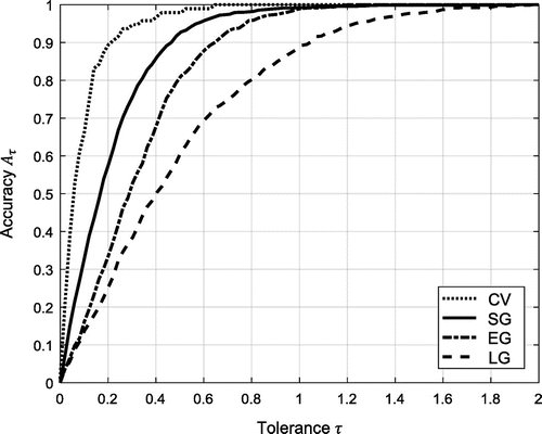
4.2. Evaluation with accuracy metric

For our first, accuracy-based evaluation perspective, we introduce a tolerance parameter for the maximal acceptable deviation between all pairs of ground truth and estimate . Given between all corresponding pairs of true and estimated swing ratios, we quantify the accuracy as follows:(10)

We sweep through increasing tolerance values in the range , expecting to see rising accuracy curves as we make the evaluation less and less strict.

In Figure 5, we illustrate the relationship between the quantities introduced above in an example with ground truth swing ratios measured at discrete points in time. As introduced in Figure 2(c), the bold black line depicts the swingogram-based swing-ratio trajectory. The black dashed lines running in parallel to the trajectory show the tolerance area whose width is determined by . For example, the error (centered at s) clearly exceeds .

In Figure 6, the dashed line shows the accuracy for condition LG, while the dash-dotted line shows the accuracy for condition EG. We can observe that the linear swing-ratio model of condition EG already yields better results than the constant model used in condition LG. However, both curves are clearly below the solid black line representing the results that can be achieved with swing ratios extracted via our proposed method (SG). Considering the dependency on the tolerance , we see that one can obtain a reasonable accuracy when accepting absolute deviations between estimated and true swing ratios up to . For the CV condition, we can see that the accuracies approach 0.85 already below .

4.3. Evaluation with root mean squared error

For the second evaluation perspective, we revert to the model assumption that our automatically estimated can be interpreted as noisy measurements of the true . We use the Root Mean Squared Error (RMSE) as a quality metric:(11)

In general, the RMSE value is unbounded but should be close to zero in case of low error.

In Figure 7, the black bars show the that is achieved for the test conditions LG, EG, and SG (using ground truth triplets). The highest error of is apparent for LG, the condition assuming a constant swing ratio . The second highest error occurs for condition EG, assuming a linear relationship between the given tempo and the swing ratio. In comparison, our swingogram-based estimates (SG) achieve . As expected, the condition CV shows the smallest error with (in gray, using ground truth triplets). It is not surprising that human experts show a certain level of disagreement when transcribing RC onsets. Aside from differences in perception, an unknown fraction of this error can also be attributed to technical inaccuracies of the tools used for manual transcription.

Figure 7. Results of our evaluation from the RMSE perspective.

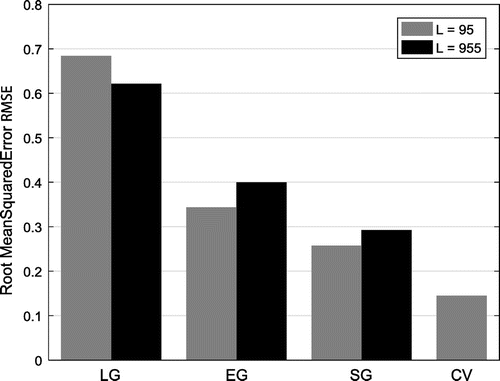
Since we only had swing-ratio pairs available for comparison in the CV case, we re-evaluated the conditions LG, EG, and SG with the same subset of ground truth triplets. In that case, as shown by the gray bars, both EG and SG show a slightly better performance, both error metrics drop by approximately 15 %. In contrast, the for condition LG even increases. This can be explained by the fact that the ground truth swing-ratios in the CV subset are more evenly distributed and less biased towards the tied-triplet feel. Overall, we can see that our proposed method for swing ratio estimation has an advantage over simpler models, although it is not on par with human performance. It remains to be seen how the general tendencies change once a larger set of manual RC annotations is available.

5. Micro-rhythm analysis in the Swingogram

In this final section, we want to explore RC swing ratios extracted from recordings of improvisations included in the WJD. First, we re-examine the relationship between tempo and swing ratio. Then, we discuss three excerpts, where preliminary observations about different strategies of micro-rhythmic interplay between soloist and drummer can be made.

5.1. Tempo vs. swing ratio

Continuing our previous work (Dittmar et al., 2015), we re-examine the much-debated relationship between tempo and swing ratio of the drummer (see Section 2.1). In Figure 8(a), we show the results from our previous paper for reference. Each point in the scatterplot is placed according to swing ratio and tempo estimated in short excerpts of recordings contained in the WJD. The different markers and colors encode the names of renowned jazz drummers who played in the excerpts under analysis. For the sake of visibility, we only depict the 10 drummers that appeared most frequently. In total, 278 excerpts with a typical duration between two and six seconds went into this figure, each of these excerpts corresponds to one pair of tempo and swing ratio. In the current paper, we can evaluate much larger quantities of swing-ratio estimates, by considering entire trajectories of swing ratios covering almost all relevant solo recordings contained in the WJD.

In Figure 8(b), we show the scatterplot that we obtain with our swingogram-based extraction of swing-ratio trajectories. Compared to Figure 8(a), it can be seen that our tempo vs. swing-ratio diagram is much more densely populated with points. A total of 67 solos³ with swing rhythm feel went into this plot, leading to 28, 851 data points. This large number results from the fact that we extract the swingogram  with a constant hop size of 250 ms between consecutive LLACF segments. The resulting swing-ratio trajectories exhibit the same temporal resolution, yielding up to 240 swing-ratio estimates per minute.

Figure 8. Tempo vs. swing ratio in the WJD. (a) Scatterplot from our previous paper (Dittmar et al., 2015). (b) Scatterplot with much higher number of tempo and swing-ratio pairs. (c) Statistical model of the same data, overlayed with hypothetic swing-ratio limits and pointers to selected examples (see Section 5.2).

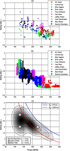
Due to the large amount of data, we decided to approach the tempo vs. swing-ratio question from a statistical modeling perspective for a better overview. To this end, we model the probability of a certain swing ratio appearing at a certain tempo by a Gaussian Mixture Model (GMM) that is fit to the data points of Figure 8(b). In Figure 8(c), we show the resulting two-dimensional probability density function as a contour plot, where darker shades of gray encode higher likelihood to observe a certain combination of tempo and swing ratio given the WJD data. We can observe in general that higher tempi lead to lower swing ratios. However, it also becomes evident that this is not a strong negative correlation but rather a wide band of possible swing ratios with increasing spread at lower tempi.

This increased variance is also visible in Figure 8(b), where there are clusters of data points that are shaped like vertical lines and appear at the same tempo (e.g. between 100 BPM and 150 BPM). Of course, the huge number of data points at a certain tempo are due to the fact that the data is taken from a limited number of recordings each of them having a definite tempo with only tiny variations. Thus, there is no statistical distribution with regard to tempo but, on the contrary, many data points accumulated at certain tempi. Note that many of the columns have different colors according to certain drummers playing on certain recordings each with an almost constant tempo.

On the other hand, the columns might also be caused by estimation errors introduced by our proposed method. Recall that we obtained an accuracy when we allowed a tolerance of (see Figure 6). This uncertainty could be an explanation for the observed line-shaped clusters, especially the ones that exhibit a swing ratio spread of around their center.

Additionally, jazz drummers might deliberately add variation to their swing ratio, especially at lower tempi, in order to make their playing more vivid and to interact with the soloist. To further investigate this phenomenon, we show the average tempo and swing ratio of three jazz excerpts corresponding to the markers in Figure 8(c). Their titles are given in the lower left legend with the standard deviation of the swing-ratio trajectory given in brackets (denoted as ). Note that the swing-ratio estimates of these three recordings are not among the data points underlying Figure 8(b). In Section 5.2, we will re-use these three examples to discuss in detail observations about the interaction between soloist and drummer. For now, it is important to note that excerpts (1) (see Section 5.2.1) and (2) (see Section 5.2.2) exhibit rather small variation in the drummer’s swing ratio, whereas excerpt (3) shows a considerable spread. As we show in Section 5.2.3, this recording features a change in the rhythmic play of both the soloist and the drummer along with a considerable drop in swing ratio. To account for this bimodal swing ratio behavior, we added two boxes to our figure, each of which is centered at the average swing ratio dominating in the different sections of this excerpt.

Finally, the red line in Figure 8(c) depicts a hypothetical swing ratio that would be caused by sweeping along the tempo axis with a fixed offbeat IOI of ms. This line was brought up by Friberg and Sundström (2002) as an upper limit to the swing ratio that can be observed in jazz music. For our data, however, the red curve cuts straight through the ridge of highest probability. Already in our previous study, we found many jazz excerpts with lower offbeat IOI, going down to ms in some rare cases. Since we manually double-checked these findings and are confident that they are not caused by extraction errors, we propose to shift the border of the hypothetical ‘no-go area’ towards the blue line corresponding to  ms.

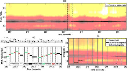
Figure 9. Swingogram analysis of a solo-section from the 1960 recording of ‘The Red Door’. See Section 5.2.1 for discussion.

5.2. Micro-rhythmic interaction between drummers and soloists

We close this paper with three observations of short excerpts taken from the WJD. In Sections 5.2.1, 5.2.2, and 5.2.3, we discuss each excerpt as a case study on how our novel swingogram can help to quickly assess the interaction between drummer and soloist. As explained in Section 2.1, we want to re-examine certain observations made by Friberg and Sundström (2002) and Benadon (2006). In essence, we are interested in three hypotheses:

(1)	Soloists tend to play with a lower swing ratio than the accompanying drummers.
(2)	Soloists try to synchronize their offbeat onsets to those of the drummers.
(3)	Soloists strive for higher swing ratios and thus better synchronization at phrase endings.

The panels in Figures 9–11 are arranged in the same fashion. In the top panel (a), we show a swingogram overlayed with the swing-ratio trajectory as introduced in Section 3.1. While panel (a) covers the complete solos (duration between 30 and 60 s), we additionally mark an excerpt of interest by vertical dashed lines. In panels (b) and (c), we provide a zoomed view into these sections, each of which are three measures long (i.e. 12 beats).

For each solo section, the lower left panel (b) provides both a score notation and a piano-roll notation of the tones played by the soloist. The vertical gray lines in the background visualize the beat grid that we directly obtain from manual annotations in the WJD. The dashed gray lines depict the corresponding offbeat positions which we computed from the automatically extracted swing-ratio trajectory. We arranged the note heads to correspond to the onsets of the piano roll objects. Furthermore, we use the same color-coding for onbeat and offbeat as introduced in Figure 1 in order to highlight the interesting eighth notes of the soloist.

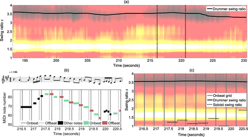
Figure 10. Swingogram analysis of a solo-section from the 1961 recording of ‘Down Under’. See Section 5.2.2 for discussion.

Finally, the lower right panel (c) provides a zoom into the swingogram. In addition to the drummer’s swing-ratio trajectory, we again depict the beat grid by vertical gray lines. On top, we indicate the swing-ratio estimates of the soloist by vertical dashed line segments. These estimates are based on the triple criterion (see Section 4.1) in combination with the annotations of the metrical position for each note as contained in the WJD. In contrast to the drummer’s swing ratio, the soloist swing ratio can only be measured when sequences of eighth notes are played.

We recommend to listen to the Youtube videos of our examples that we provide on our accompanying webpage.⁴ During playback, a synchronized cursor highlights the current position within the swingogram as well as the piano-roll notation of the solos. Some of the phenomena discussed below are clarified by listening to the music examples.

5.2.1. The red door

In Figure 9, we analyze an excerpt from ‘The Red Door’, recorded by the Gerry Mulligan group in 1960, in order to study the micro-rhythmic interplay of solo baritone saxophonist Gerry Mulligan and drummer Mel Lewis. In Figure 9(a), it can be observed that Lewis keeps the idealized tied triplet swing ratio for more than 60 s at an average tempo of 236 BPM. Mulligan plays in the same precise fashion, almost always synchronizing his onbeat onsets to those of Lewis. However, he shows quite some variability in his offbeat onsets, indeed showing higher swing ratio at phrase endings, as hypothesized by Benadon (2006).

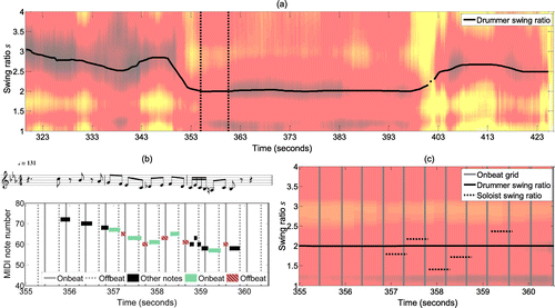
Figure 11. Swingogram analysis of a solo-section from the 1957 recording of ‘Blue Train’. See Section 5.2.3 for discussion.

5.2.2. Down under

In Figure 10, we show a solo section from ‘Down Under,’ recorded by Art Blakey’s Jazz Messengers in 1961, with trumpet player Freddie Hubbard performing together with drummer and bandleader Art Blakey. At an average tempo of 146 BPM, the RC swing ratio exhibits a slightly wavy variation around . This gives an example of the archetype of drummers playing high swing ratios at low tempi as discussed in Section 5.1. In contrast, Hubbard stays at the other end of the swing-ratio range at around in the zoomed-in section. Furthermore, one can clearly see that Hubbard plays his onbeat onsets in a laid-back fashion behind the beat grid. His offbeats, however, synchronize very well to Blakey’s offbeats most of the time as hypothesized by Friberg and Sundström (2002).

5.2.3. Blue train

In Figure 11, we present an excerpt from John Coltrane’s recording ‘Blue Train,’ (1975) featuring solo trombone player Curtis Fuller and drummer Philly Joe Jones. At an average tempo of 132 BPM, the RC swing ratio starts around and drops in the middle part to . The change in swing ratio is coupled with the start of a completely different drum pattern. In contrast to our previous, well-behaved examples, the RC plays only onbeats (i.e. quarter notes), while the HH is placed on straight offbeats, thus conveying a double-time feel (i.e. the impression of twice the tempo). On closer inspection, we found that swinging eighths notes in the middle part are played solely on the snare. Still, the snare hits lead to spikes in the novelty curve due to crosstalk into the RC frequency band.

Interestingly, both the bassist Paul Chambers and trombonist Curtis Fuller do not follow the rhythm change immediately. This might explain the rather loose interplay during the excerpt where neither the onbeats nor the offbeats played on the trombone synchronize particularly well to the drummer. Instead, the soloist’s swing ratio oscillates around the drummer’s swing ratio. However, shortly after the end of our zoomed section, Fuller switches to sixteenth note sequences, supporting the double time feel.

6. Conclusions and future work

In this paper, we introduced the swingogram, a novel time vs. swing-ratio representation suited for analyzing the time-varying behavior of swing ratios in jazz solo recordings. We evaluated the accuracy of our semi-automatic swing-ratio estimates by comparing them against ground-truth annotations using two different evaluation metrics. We revisited the debated linear relationship between tempo and swing ratio that has been in the scope of several researchers. Thanks to our swing-ratio estimation method and the availability of the WJD corpus, we were able to base our analysis on a considerably larger collection than previous studies. This lead to new insights about the probability density distribution of swing ratios in different tempo ranges as well as the hypothetic upper limit to swing ratios. Using three examples from the WJD, we illustrated how our swingogram visualization can support the understanding of the interaction between the soloist and the drummer. This immediate access to interesting solo sections is of pivotal interest for a comprehensive analysis of micro-rhythm within a jazz performance.

Future work will be directed towards investigating the interaction between drummer and soloist as discussed by Friberg and Sundström (2002) on a larger scale. In principle, sufficient data sources required to allow statistical evaluations of their hypotheses are available. However, in the current state, some important intermediate steps are difficult to automate. The identification of soloist triples in ambiguous cases remains challenging, as well as the automatic rejection of inadequate swing-ratio trajectories in the swingogram.

From the viewpoint of signal processing, we plan to investigate the advantages and disadvantages of the LLACF-based swingogram against other extraction methods such as the scale transform (Holzapfel & Stylianou, 2011) or the shift-ACF (Kurth, 2013). At this point, it seems promising to also apply these methods for the analysis of other micro-rhythmic phenomena, such as shuffle or groove, too.

Acknowledgements

The authors would like to thank all student assistants participating in the transcription and annotation process for the WJD. The International Audio Laboratories Erlangen is a joint institution of the Friedrich-Alexander-Universität Erlangen-Nürnberg (FAU) and the Fraunhofer-Institut für Integrierte Schaltungen IIS.

Additional information

Funding

The JAZZOMAT RESEARCH PROJECT is supported by the German Research Foundation (DFG-PF 669/7-1). Christian Dittmar is supported by the German Research Foundation (DFG-MU 2686/10-1).

Notes

No potential conflict of interest was reported by the authors.

1 https://www.audiolabs-erlangen.de/resources/MIR/2017-JNMR-SwingRatio.

2 http://jazzomat.hfm-weimar.de/dbformat/dboverview.html.

3 The metadata for these solos are provided on our accompanying webpage: https://www.audiolabs-erlangen.de/resources/MIR/2017-JNMR-SwingRatio.

4 https://www.audiolabs-erlangen.de/resources/MIR/2017-JNMR-SwingRatio.

References

- Bartsch, M. A. , & Wakefield, G. H. (2005). Audio thumbnailing of popular music using chroma-based representations. IEEE Transactions on Multimedia , 7 , 96–104.
- Benadon, F. (2006). Slicing the beat: Jazz eighth-notes as expressive microrhythm. Ethnomusicology , 50 , 73–98.
- Berliner, P. F. (1994). Thinking in Jazz: The infinite art of improvisation . Chicago: University of Chicago Press.
- Böck, S. , Arzt, A. , Krebs, F. , & Schedl, M. (2012). Online real-time onset detection with recurrent neural networks. In Proceedings of the International Conference on Digital Audio Effects (DAFx) , York, UK.
- Busse, W. G. (2002). Toward objective measurement and evaluation of jazz piano performance via MIDI-based groove quantize templates. Music Perception , 19 , 443–461.
- Cannam, C. , Landone, C. , & Sandler, M. B. (2010). Sonic visualiser: An open source application for viewing, analysing, and annotating music audio files. In Proceedings of the International Conference on Multimedia (pp. 1467–1468). Florence, Italy.
- Collier, G. L. , & Collier, J. L. (2002). A study of timing in two louis armstrong solos. Music Perception , 19 , 463–483.
- Davies, M. , Madison, G. , Silva, P. , & Gouyon, F. (2013). The effect of microtiming deviations on the perception of groove in short rhythms. Music Perception , 30 , 497–510.
- Dittmar, C. , & Gärtner, D. (2014). Real-time transcription and separation of drum recordings based on NMF decomposition. In Proceedings of the International Conference on Digital Audio Effects (DAFx) (pp. 187–194). Erlangen, Germany.
- Dittmar, C. , Pfleiderer, M. , & Müller, M. (2015). Automated estimation of ride cymbal swing ratios in jazz recordings. In Proceedings of the International Conference on Music Information Retrieval (ISMIR) (pp. 271–277). Málaga, Spain.
- Dixon, S. (2006). Onset detection revisited. In Proceedings of the International Conference on Digital Audio Effects (DAFx) (pp. 133–137). Montreal, Quebec, Canada.
- Dixon, S. , Gouyon, F. , & Widmer, G. (2004). Towards characterisation of music via rhythmic patterns. In Proceedings of the International Society for Music Information Retrieval Conference (ISMIR) (pp. 509–516). Barcelona, Spain.
- Ellis, D. P. (2007). Beat tracking by dynamic programming. Journal of New Music Research , 36 , 51–60.
- Ellis, M. C. (1991). An analysis of ‘swing’ subdivision and asynchronization in three jazz saxophonists. Perceptual and Motor Skills , 73 , 707–713.
- Eppler, A. , Männchen, A. , Abeßer, J. , Weiß, C. , & Frieler, K. (2014). Automatic style classification of jazz records with respect to rhythm, tempo, and tonality. In Proceedings of the Conference on Interdisciplinary Musicology (CIM) , Berlin, Germany.
- Eyben, F. , Böck, S. , Schuller, B. , & Graves, A. (2010). Universal onset detection with bidirectional long short-term memory neural networks. In Proceedings of the International Society for Music Information Retrieval Conference (ISMIR) (pp. 589–594). Utrecht, The Netherlands.
- Foote, J. , & Uchihashi, S. (2001). The beat spectrum: A new approach to rhythm analysis. In Proceedings of the International Conference on Multimedia and Expo (ICME) , Los Alamitos, CL, USA.
- Friberg, A. , & Sundström, A. (2002). Swing ratios and ensemble timing in jazz performance: Evidence for a common rhythmic pattern. Music Perception , 19 , 333–349.
- Frieler, K. , Zaddach, W.-G. , Abeßer, J. , & Pfleiderer, M. (2013). Introducing the jazzomat project and the melospy library. In Third International Workshop on Folk Music Analysis , Amsterdam, The Netherlands.
- Grosche, P. , & Müller, M. (2011a). Extracting predominant local pulse information from music recordings. IEEE Transactions on Audio, Speech, and Language Processing , 19 , 1688–1701.
- Grosche, P. , & Müller, M. (2011b). Tempogram toolbox: MATLAB tempo and pulse analysis of music recordings. In Late-Breaking and Demo Session of the International Conference on Music Information Retrieval (ISMIR) . Miami, FL, USA.
- Gruhne, M. , & Dittmar, C. (2009). Improving rhythmic pattern features based on logarithmic preprocessing. In Proceedings of the Audio Engineering Society (AES) Convention , Munich, Germany.
- Holzapfel, A. , & Stylianou, Y. (2009). A scale transform based method for rhythmic similarity of music. In Proceedings of the IEEE International Conference on Acoustics, Speech, and Signal Processing (ICASSP) (pp. 317–320). Taipei, Taiwan.
- Holzapfel, A. , & Stylianou, Y. (2011). Scale transform in rhythmic similarity of music. IEEE Transactions on Audio, Speech, and Language Processing , 19 , 176–185.
- Honing, H. , & de Haas, W. B. (2008). Swing once more: Relating timing and tempo in expert jazz drumming. Music Perception: An Interdisciplinary Journal , 25 , 471–476.
- Jensen, J. H. , Christensen, M. G. , & Jensen, S. H. (2009). A tempo-insensitive representation of rhythmic patterns. In Proceedings of the European Signal Processing Conference (EUSIPCO) (pp. 1509–1512). Glasgow, Scotland.
- Jensen, K. (2006). Multiple scale music segmentation using rhythm, timbre, and harmony. EURASIP Journal on Advances in Signal Processing , 2007 , 1–11.
- Kerschbaumer, F. (1978). Miles Davis: Stilkritische Untersuchungen zur musikalischen Entwicklung seines Personalstils . Graz: Studies in jazz research. Akademische Druck und Verlagsanstalt.
- Kurth, F. (2013). The shift-ACF Detecting multiply repeated signal components. In Proceedings of the IEEE Workshop on Applications of Signal Processing to Audio and Acoustics (WASPAA) (pp. 1–4). New Paltz, NY, USA.
- Kurth, F. , Gehrmann, T. , & Müller, M. (2006). The cyclic beat spectrum: Tempo-related audio features for time-scale invariant audio identification. In Proceedings of the International Conference on Music Information Retrieval (ISMIR) (pp. 35–40). Victoria, Canada.
- Marchand, U. , & Peeters, G. (2014). The modulation scale spectrum and its application to rhythm-content description. In Proceedings of the International Conference on Digital Audio Effects (DAFx) (pp. 167–172). Erlangen, Germany.
- Marchand, U. , & Peeters, G. (2015). Swing ratio estimation. In Proceedings of the International Conference on Digital Audio Effects (DAFx) (pp. 423–428). Trondheim, Norway.
- Müller, M. (2015). Fundamentals of music processing . Heidelberg: Springer Verlag.
- Parsons, W. , & Cholakis, E. (1995). It don’t mean a thing if it ain’t dang, dang-a dang!. Downbeat , 52 , 61.
- Peeters, G. (2005). Rhythm classification using spectral rhythm patterns. In Proceedings of the International Society for Music Information Retrieval Conference (ISMIR) (pp. 644–647). London, UK.
- Pfleiderer, M. (2006). Rhythmus: Psychologische, theoretische und stilanalytische Aspekte populärer Musik . Bielefeld: Transcript.
- Prockup, M. , Ehmann, A. F. , Gouyon, F. , Schmidt, E. M. , & Kim, Y. E. (2015). Modeling musical rhythm at scale with the music genome project. In Proceedings of the IEEE Workshop on Applications of Signal Processing to Audio and Acoustics (WASPAA) . New Paltz, NY, USA.
- Reinholdsson, P. (1987). Approaching jazz performances empirically. some reflections on methods and problems. Action and Perception in Rhythm and Music , 55 , 105–125.
- Rioul, O. , & Vetterli, M. (1991). Wavelets and signal processing. IEEE Signal Processing Magazine , 8 , 14–38.
- Röbel, A. , Pons, J. , Liuni, M. , & Lagrange, M. (2015). On automatic drum transcription using non-negative matrix deconvolution and itakura saito divergence. In Proceedings of the IEEE International Conference on Acoustics, Speech and Signal Processing (ICASSP (pp. 414–418). Brisbane, Australia.
- Rose, R. F. (1989). An analysis of timing in jazz rhythm section performances, PhD thesis, University of Texas.
- Southall, C. , Stables, R. , & Hockman, J. (2016). Automatic drum transcription using bi-directional recurrent neural networks. In Proceedings of the International Society for Music Information Retrieval Conference (ISMIR) (pp. 591–597). New York City, NY.
- Sturm, B. L. (2012). An analysis of the GTZAN music genre dataset. In Proceedings of the International ACM Workshop on Music Information Retrieval with User-Centered and Multimodal Strategies MIRUM (pp. 7–12). Nara, Japan.
- Vogl, R. , Dorfer, M. , & Knees, P. (2017). Drum transcription from polyphonic music with recurrent neural networks. In Proceedings of the IEEE International Conference on Acoustics, Speech, and Signal Processing (ICASSP) (pp. 201–205). New Orleans, LA, USA.
- Völkel, T. , Abeßer, J. , Dittmar, C. , & Großmann, H. (2010). Automatic genre classification on latin music using characteristic rhythmic patterns. In Proceedings of the Audio Mostly : A Conference on Interaction with Sound , Piteå, Sweden.
- Wesolowski, B. C. (2012). Testing a model of jazz rhythm: Validating a microstructural swing paradigm, PhD thesis, University of Miami, Miami, FL, USA.
- Wu, C.-W. , & Lerch, A. (2015). Drum transcription using partially fixed non-negative matrix factorization with template adaptation. In Proceedings of the International Society for Music Information Retrieval Conference (ISMIR) (pp. 257–263). Málaga, Spain.