Graininess characterization by multidimensional scaling

ABSTRACT

A validation of the graininess attribute was made by means of a psychophysical experiment and the multidimensional scaling algorithm. A visual experiment was designed to obtain graininess differences to be used like the dissimilarity matrix in the MDS algorithm. The results revealed that two dimensions are needed to characterize the graininess effect. The BYK-mac-i instrument and a gonio-hyperspectral imaging system were employed to evaluate the statistical dimensions. On one hand, the first dimension correlated well with the graininess value provided by the BYK-mac-i (r² = 0.9566). However, we were unable to find a relationship with dimension 2 and any parameter measured by this instrument. Furthermore, the images captured by the gonio-hyperspectral imaging system were processed. A good relationship with the correlation parameter was observed (r² = 0.8958). However, no relationship was established with dimension 2. Based on these conclusions, further research is necessary that focuses on the new imaging processes and a new visual experiment.

KEYWORDS:

• Graininess
• special-effect pigments
• multidimensional scaling algorithm
• psychophysical experiment

1. Introduction

The visual appearance of a product is important for different reasons. On the one hand, visual appearance allows the manufacturer to know about the reproducibility of its production; i.e. it is an index of the quality control level. In different industrial sectors (leather, glass, cosmetics, ceramics, printed materials, etc.), the final quality control is still done by making visual observations because measurement systems have not yet reached the required level of sensitivity. On the other hand, the visual appearance of a product is a critical parameter implicated in customers’ purchase decisions. For these reasons, in recent years, many different efforts have been made by industrial manufacturers to provide attractive and sophisticated visual effects by using, for instance, goniochromatic pigments (1–5).

Goniochromatism is defined as an abrupt colour change due to the light source and observer angle variations. In this way, it is possible to distinguish among lightness variations due to metallic pigments (flakes), and hue and chroma variations due to pearlescent or diffraction pigments. Besides this angular dependence on viewing/illumination direction, special-effect pigments also exhibit a visually complex texture. Depending on the properties of the finish, and also on the viewing and illumination conditions, flakes can exhibit a distinct spatial appearance (6–8).

Under bright direct illumination conditions, such as bright sunlight, the flakes in a metallic finish glitter create a sparkling effect. Tiny bright sparkles of light that vary in intensity can be seen, like stars in the night sky. This effect is known as sparkle. Sparkle is observed only at close distances and under bright direct illumination. On the other hand, with diffuse illumination, such as a cloudy sky, metallic finishes do not sparkle. Instead, they may create a salt-and-pepper appearance. This effect may be referred to as graininess or coarseness. In particular, graininess or diffuse coarseness is the perceived contrast of the light/dark irregular pattern on a scale of <100 µm (7, 8). Thus in order to visualize the graininess effect, it is necessary to use diffuse illumination and close observation distance; however, they are independent of the observation angle. Both sparkle and graininess depend on flake size, orientation and distribution (9–11). Metallic finishes with larger coarse flakes show an intense sparkle, while those with very fine flakes appear uniform, almost like a solid colour.

Nowadays, there is only one instrument on the market able to measure the effects of texture, the multi-angle spectrophotometer BYK-mac (12). This instrument measures colour at six measurement geometries and includes a CCD monochrome camera to measure texture effects. To measure the sparkle effect, the sample is illuminated directionally under 15°, 45° and 75°, counted to the normal direction from the sample surface. Three parameters are obtained to characterize sparkle, sparkle intensity (Si), sparkle area (Sa) and sparkle grade (SG), for the three directional geometries. The total size of the small and bright areas per unit area is called the sparkle area. Sparkle intensity is specified as the intensity of the small bright light spots in relation to the intensity of the surrounding less bright. Sparkle area and sparkle intensity are combined in the representative sparkle attribute called sparkle grade (6, 7, 13). To measure the graininess effect, the sample is diffusely illuminated by an integrating sphere. To evaluate or measure graininess, the non-uniformity of the light/dark areas is evaluated. These areas are recorded by the CCD camera, which provides a gray-scale picture. The uniformity of this image is a measurement of graininess. Therefore, a higher graininess value means an image with less uniformity. Graininess is the sum of all the reflections in relation to a uniformly reference coating and is finally defined by a relative value (G) (6).

However, there are no standards like ISO, ASTM or DIN which propose the mathematical and optical algorithms required to measure and calculate the sparkle or graininess effect implemented by the BYK-Gardner company. Therefore, it is very important to visually validate the sparkle and graininess effects in psychophysical experiments as these texture effects are important for the visual discrimination of many materials and quality control (13).

In recent years, several studies have been carried out to visually evaluate texture effects. This has led some hypotheses widely discussed among the scientific community (e.g. in the CIE technical committee JTC 12 ‘The measurement of sparkle and graininess’) suggesting that the graininess effect is not well characterized with a unique variable, but instead more variables or parameters are needed. However, a recent paper was published to propose traceable graininess measurements (14). In this article, it is concluded that the average luminance factor should be considered, and it is proposed as the second relevant reflectance-based quantity for the quantification of graininess.

The multidimensional scaling (MDS) technique allows multivariate relationships or dimensions to be determined to characterize an attribute (15–17). MDS shows the perceived distances, orders or similarities among stimuli as spatial maps. That is, a configuration of n points representing the objects is distributed in a p dimensional space. Each point represents one object. Between pairs of points (i, j) there is a distance that is not necessarily Euclidean, d_ij. Thus the aim of MDS is to find a configuration in such a way that distances d_ij match the previously measured dissimilarities x_ij. Therefore, similar stimuli are located together, whereas different stimuli are far away. No previous knowledge about the number of dimensions is required to apply this algorithm. However, it is necessary to figure out the meaning of the dimensions after the analysis; that is, what they represent in terms of perceptual and physical attributes rather than as mathematical correlates. As input, the distance or dissimilarity between stimuli has to be computed. The experimenter can choose the method to establish disparities. The advantage of combining this algorithm with visual perception is to quantify this distance by psychophysical experiments.

Therefore, this technique determines a set of vectors in a p-dimensional space, like those that correspond to the matrix of Euclidean distances, that comes as close as possible to a function of the input matrix according to a criterion parameter called stress. Stress is a parameter that defines the degree of correspondence between the dissimilarities among the points in input data (X) measured by observers. The stress parameter is calculated by the following equation: (1) $\text{stress}=\sqrt{\frac{{\sum \sum \left(x_{ij}-d_{ij}\right)}^2}{\sum d_{ij}^2}}$(1) In the equation, d_ij is the Euclidean distance across all the dimensions between points i and j on the spatial map. Therefore, a lower stress value means a better representation. The algorithm can be described as follows:

1. assign points to the arbitrary coordinates in a p-dimensional space;

2. calculate Euclidean distances among all the pairs of points to obtain the D matrix;

3. compare the D matrix with the input X matrix by evaluating the stress parameter;

4. adjust the coordinates of each point to optimize the stress value;

5. repeat steps 2 through to 4 until stress is stabilized.

Therefore, the objective of this work is to evaluate the graininess effect to find how many dimensions are needed to totally characterize this texture effect by multidimensional scaling after taking into account observers’ visual perception. Following this idea, Wang and Luo (18) conducted different visual experiments to evaluate the texture perception on special coatings. They found a correlation between the instrumental and the visual graininess by using a second-order polynomial model. However, the MDS technique was only applied to establish the dimensions for the glint/sparkle space.

2. Materials and methods

The visual experiment to scale graininess differences was based on the interval method (point-rating scaling). The question that observers were asked was: how much do these two samples differ in graininess? The difference was specified on a line: the start point marked 0 and an endpoint marked +++. The starting point (0) means there is no difference between samples. The endpoint (+++) means the difference between samples is very big. This method was used to avoid any verbalization of answers as it can imply misunderstanding the interpretation. Observers indicated the perceived difference of the pair presented on the line by a mark (x). To quantify the perceived difference, the distance between the starting point (0) and the observer’s mark (x) was measured. Each observer performed three repetitions after a training session. During this training session, the panels with a maximum difference in graininess were shown to the observers to raise awareness and to stabilize their answers. Seventeen observers participated in the experiment (11 males and 6 females). Their average age was 33 years old. All the observers who participated in the experiment had a best-corrected visual acuity of 1 (decimal scale).

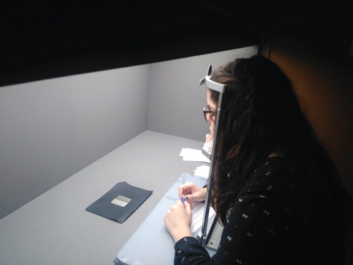
A VeriVide viewing booth was used to run the experiment (Figure 1). Illumination was quite diffuse and it was not possible to perceive sparkle on the samples. The selected illuminant was the D65 illuminant. The colorimetric properties of this light source were measured by a Photo Research PR-650 tele-spectroradiometer. The measured chromatic coordinates were of x = 0.3127 and y = 0.3383. The correlated colour temperature equalled 6439 K, with a colour rendering index, Ra, of around 95 units. The experiment was conducted in a dark room and the observers took 3 min to adapt to the lightness conditions.

Figure 1. Setup of the visual experiment.

A set of 25 samples was selected to run the experiment. These samples belong to the Effect Navigator® chart from Standox (Figure 2). This chart was developed to select the exact flake size (texture effect) for colour matching in the car refinishing industry. Samples are painted in cardboard (size: 70 × 120 mm), composed of five different grades of lightness and effect. Two different instruments were used to characterize samples. The BYK-mac-i multi-angle spectrophotometer was used to obtain the CIELAB values under the D65 illuminant at six different measurement geometries. In addition, the texture of samples was determined by the sparkle (Sa, Si, and SG) and graininess (G) parameters, which were provided by this instrument. The measuring area of this instrument had a 23-mm diameter. Furthermore, a gonio-hyperspectral imaging system, developed in the Centre for Sensors, Instruments and Systems Development (CD6) at the Universitat Politècnica de Catalunya, was used to acquire images with high spatial resolution to evaluate graininess. The system characterizes samples by their spectral reflectance, and colour at different geometries, and also through the textural effects of sparkle, graininess and mottling. Regarding textural measurements, the graininess attribute is defined by specific indices, based mainly on first- and second-order statistics (19, 20). The measuring area of this instrument was of 50 × 37 mm.

Figure 2. The set of samples (Effect Navigator chart) used in the visual experiment. From top to bottom: L1 (lighter) to L5 (darker). From left to right: increasing flake size.

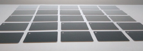
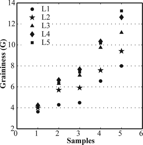
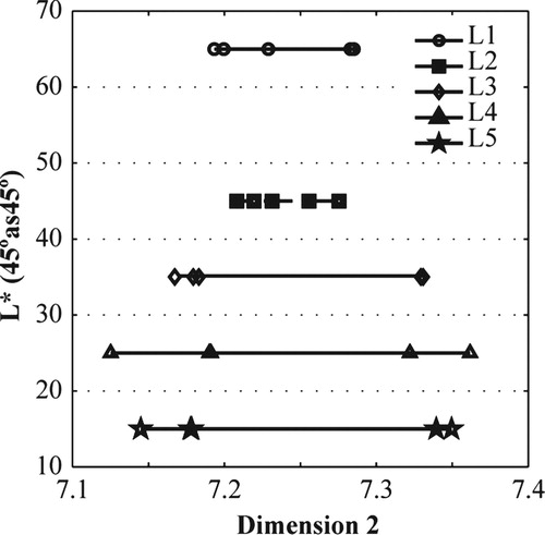
The lightness or colour background of samples can influence the graininess perception. For this reason, the selected samples were achromatic samples ($C_{ab}^{\ast }<10$) and were divided into different groups after taking into account the lightness value. This classification avoided other contributions to the graininess perception. Thus the samples used for this experiment were divided into five groups according to the lightness value for the 45°as45° measurement geometry. That is, the illumination angle was 45° regarding the normal direction from the sample, and the measurement or observation angle was 45° regarding the specular direction, or 0° regarding the normal direction from the sample. This measurement geometry was considered to come closer to the illumination and viewing conditions inside the lighting booth used for the visual experiment. In each one, there were five samples with a different graininess value, ranging from a weak to strong graininess effect (Figure 3): $\begin{array}{r}\text{L}1:L^{\ast }=60,Gϵ\left[3.5,8\right]\\ \text{L}2:L^{\ast }=45,Gϵ\left[4,9.5\right]\\ \text{L}3:L^{\ast }=35,Gϵ\left[4,11\right]\\ \text{L}4:L^{\ast }=25,Gϵ\left[4,12.5\right]\\ \text{L}5:L^{\ast }=15,Gϵ\left[4,13\right]\end{array}$

Figure 3. The graininess value measured by the BYK-mac-i instrument for the set of samples used in this experiment.

Therefore, 10 different pairs per group were compared. Then each observer made 50 visual assessments during a 30-min session to avoid fatigue. Three different sessions per repetition were run. For this visual experiment, 2250 visual assessments were made.

The visual experiment was designed to obtain dissimilarities. In this way, the dissimilarity matrix could be computed to apply MDS. Therefore, the input matrix (D) for MDS was that built according to the observer’s answer; that is, perceived visual differences in graininess. This matrix was square and symmetric, which indicates relationships among samples. In fact, it was a dissimilarity matrix as a higher value means less similarity. The multidimensional analysis was implemented with Matlab® by using the mdscale function.

3. Results

The Results section is structured as follows: first, the outcomes of the visual experiment were analysed. Observer intra- and inter-variability was studied to know the consistency of the input data for the MDS algorithm. Second, the multidimensional analysis was carried out to evaluate the minimum number of dimensions needed to define or characterize the graininess attribute. Finally, the correlation between the mathematical dimensions and the physical or perceptual attributes of graininess was studied.

3.1. Intra- and inter-variability analysis

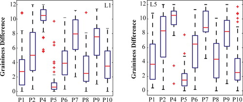
Intra-observer variability refers to the differences between the results obtained in each repetition conducted by an observer. Inter-observer variability refers to differences between the results obtained by several observers. To analyse both intra- and inter-variability, different tests of normality were applied, which were carried out with a 95% confidence level. After checking each participant’s results, it was concluded that the data were not distributed normally. The obtained p-values were always lower than the level of significance (α = 0. 05). For instance, for one observer, the Pearson Chi-Square normality test provided a p-value of 2.873e−11, while that of the Lilliefors (Kolmogorov–Smirnov) test was of 6.436e−5. Therefore, the final answer of each observer was calculated by the median of the three repetitions. Similarly, inter-variability was analysed by the same procedure. As expected, observers’ responses were not adjusted to a normal distribution (p-value = .00064 for the Pearson Chi-Square normality test and p-value = .00937 for the Lilliefors test). For this reason, instead of computing the observer average, the median was also calculated. These results were obtained for all the considered groups (L1–5) and for all the evaluated pairs. To visualize this behaviour, Figure 4 shows the box plot of the results for two lightness profiles (L1 and L5). The bottom and top of the box are the first and third quartiles, and the red line inside corresponds to the median. The ends of whiskers represent the minimum and maximum values of all the data. Any data not included between the whiskers were plotted as an outlier with a sum symbol (+). These results corroborate the previous ones obtained with the tests of normality: distribution was not normal.

Figure 4. Box plot for each pair for two lightness profiles. Left: light samples (L1); right: dark samples (L5).

3.2. MDS analysis

The mdscale function performs non-metric MDS on the dissimilarity matrix D obtained by the previously described visual experiment. As a result, the Y matrix was obtained with information on P dimensions. Scaling was computed by minimizing the stress parameter defined in the Introduction. This analysis was carried out for each lightness level.

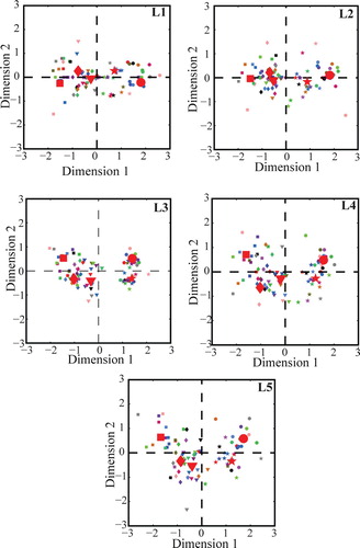
First, the analysis explained how input data were distributed in a n-dimensional space, which is useful for determining the number of dimensions needed for the graininess characterization. In Figure 5, data are shown in the two-dimensional space. The red symbols correspond to the median observer (calculated as the median value of observers). The other symbols are the individual answers provided by each observer. The scatter obtained in this figure corresponds to the variability between observers shown in the previous section. As seen, data were not distributed normally but, in standard deviation terms, a mean value of 1.2 was obtained. This value proved good to continue with further correlations. It is important to mention that observers were quite consistent at evaluating samples with high lightness or low graininess, which is why there were more scattered samples for L4 and L5. From this figure, it would appear that two dimensions were needed to define the graininess attribute, especially for the dark lightness levels (L3–L5). However, for the light lightness levels (L* > 45), one property was used mainly by considering the observers’ median value. For instance, the variation of D2 was only approximately 1/4 of the variation of D1 for L1 and L2, whereas it was ½ of D1 for L3–L5. One reason for this could be the influence of the panel set itself. The set or size of the dark and light patterns could vary within this set, but could not for the other two. Nevertheless, apparently the most important reason was that this dark and light pattern was more evident in dark samples (greater contrast). Therefore, observers could visualize a second property on this pattern much better.

Figure 5. Data dispersion in statistical dimensions for the graininess attribute evaluated by a visual experiment.

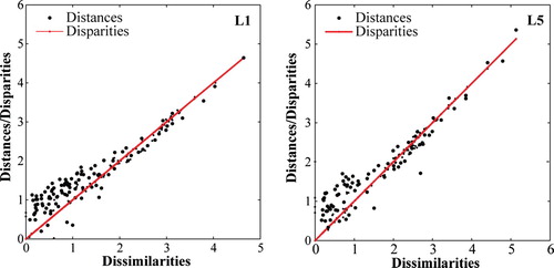
The visual differences (dissimilarities) with the disparities (or distances) obtained by the multidimensional analysis were compared. Figure 6 shows two lightness levels (L1 and L5). The black dots correspond to the dissimilarities made by observers with the visual experiment versus the distances predicted by applying MDS. The red dots correspond to the transformed dissimilarities versus predicted distances. This diagram is called a Shepard diagram and indicates the goodness of MDS. We can see that the visual differences were rather well adjusted to the distances calculated by applying MDS. Two different linear adjustments were made. The first was made by imposing the intersection on 0, and the other one was made with no restriction. The results associated with both analyses were similar for all the lightness profiles. For the first analysis, the average correlation coefficient equalled 0.8496 ± 0.0206. The average slope was 1.0077 ± 0.0058. This means that the multidimensional technique goodness was quite good as the visual differences were similar to the differences predicted/calculated by the model. However, the data dispersion was wider when the differences in graininess were smaller. For this reason, the second adjustment was made. In this case, the average correlation coefficient was 0.9294 ± 0.0115. The obtained slope equalled 0.8076 ± 0.0083 and the constant parameter equalled 0.4758 ± 0.0178. The model predicted by the multidimensional analysis overestimates the small graininess differences; that is, the MDS technique was more sensitive to small graininess differences than the visual graininess established by the observers. Generally speaking, the MDS goodness was excellent when considering the Shepard diagram.

Figure 6. Comparison between the visual differences (dissimilarities) and disparities calculated with the MDS analysis. Left: light samples (L* = 60); right: dark samples (L* = 15).

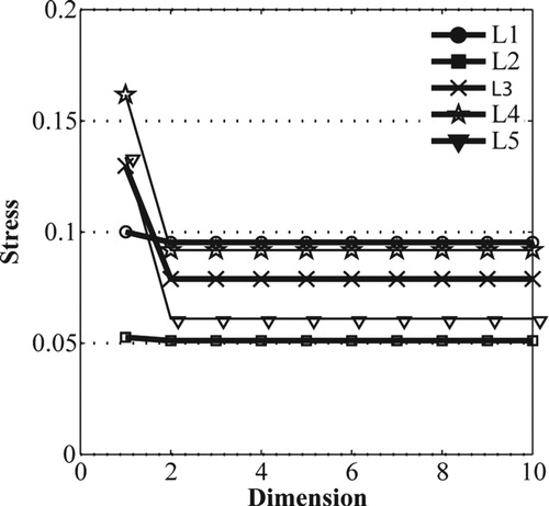
Mathematically, any dataset can be described using n − 1 dimensions, where n is the number of items to be scaled. However, if the number of dimensions increases, stress must either decrease or remain constant. Therefore, true data dimensionality or the minimum number of dimensions to perfectly describe an attribute is based on the minimum stress value. For this reason, the relationship between MDS-Dimensions and the stress parameter was evaluated by Screeplot (MDS-Dimension vs. Stress). Screeplot shows that two dimensions are needed to define the graininess attribute (Figure 7). The stress value is constant over dimension 2. Even though the results do not reach a zero value, stress values under 0.1 are considered excellent, which means that there are no random measurement errors.

Figure 7. MDS-Dimension vs. Stress according to the lightness value.

3.3. Relationship between mathematical dimensions and physical attributes

The next step was to identify the relationship between the statistical dimensions found in the previous section and some measuring parameters. First, the graininess value provided by the BYK-mac-i instrument was considered.

Before studying this correlation, the best alignment with the graininess value was obtained by rotating the D1/D2 space. It is noteworthy that the major axes obtained from an MDS are linked to an arbitrary orientation (distances remain constant by rotations). The method used to optimize the D1/D2 space was the Procrustes rotation method. The procrustes function in Matlab® was used. This function determines a linear transformation (translation, reflection, orthogonal rotation, and scaling) of the points in matrix Y (D1/D2) to best fit them to the points in matrix X (G). The criterion used to optimize the alignment was the sum of squared errors.

In Figure 8, both dimensions, 1 and 2 are compared with the graininess value obtained with the BYK-mac-i instrument. From Figure 8(a), we can observe that dimension 1 adjusts quite well to the instrumental value of the graininess attribute measured by the BYK-mac-i instrument. The correlation coefficient was calculated for each lightness profile and a mean value of r² = 0.9566 was obtained. The graininess attribute was also found to depend on the lightness value: i.e. more graininess for darker samples of the same pigment size. However, no relationship was found with dimension 2 (Figure 8(b)).

Figure 8. Relationship between the statistical dimensions and the graininess parameter calculated by the BYK-mac-i multi-angle spectrophotometer. (a) Dimension 1 vs. G_BYK-mac. (b) Dimension 2 vs. G_BYK-mac.

Therefore, other attempts were made to figure out the meaning of the second dimension. In a first attempt, the lightness value was considered to be associated with the 45°as45° measurement geometry to establish a relationship with the second dimension. Figure 9 shows the relationship between both parameters. As seen, it was not possible to find any relationship between these parameters. A similar behaviour was found for other measuring parameters, such as sparkle grade, sparkle intensity or sparkle area for the 45°as45° measurement geometry.

Figure 9. Relationship between statistical dimension 2 and lightness value L* for the 45°as45° measurement geometry.

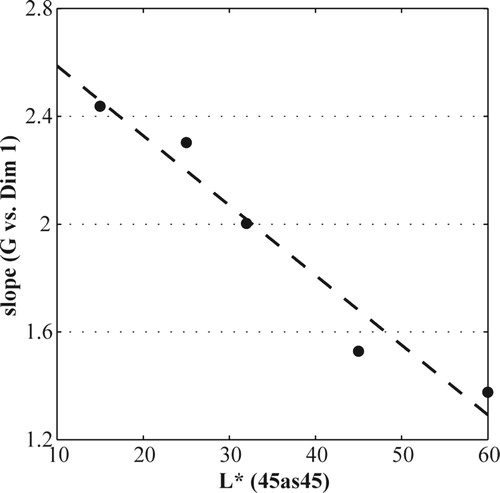
In Figure 10, the slope computed for G vs. Dim. 1 is plotted against the lightness value for the 45°as45° measurement geometry, and the calculated correlation coefficient is r² = 0.9521. The samples with the same graininess grade (high), but with different lightness, have a different dark–light pattern, which means a greater graininess perception for dark samples. Therefore, it is clear that the dark–light pattern (graininess perception) was strongly influenced by the lightness value of the samples. However, this dependency was not obtained by the dimension 2 deduced by the visual experiment conducted herein. Therefore, these results are useful for continuing to working in this field in an attempt to propose a standardized protocol to measure graininess perception by considering the influential structural or physical variables on graininess perception (pigment size and lightness value).

Figure 10. Relationship between statistical lightness value L* for the 45° as 45° measurement geometry and the slope computed for G vs. Dim. 1.

Finally, the measuring parameters calculated with the gonio-hyperspectral system were compared with the two dimensions obtained in MDS. In particular, the system provided first- and second-order statistics, such as entropy, energy and asymmetry for the first order (21–24), and contrast, correlation, energy and homogeneity for the second order (21–25). Before studying any correlation, the Procrustes rotation method was applied to the D1/D2 space to optimize the alignment between parameters. The parameter that showed a better correlation with the first dimension was the correlation parameter (Figure 11). The correlation parameter describes the digital-level linear dependencies in the image, and reaches values from −1 to 1, which are perfectly positively or negatively correlated at 1 or −1, respectively. A constant image results in an undefined correlation that equals 0. This comparison gave a mean correlation coefficient of r² = 0.8958. As the graininess effect was defined as a light–dark pattern, it proved reasonable to find a good correlation with the correlation parameter.

Figure 11. The relationship between the first dimension and the correlation parameter calculated by the gonio-hyperspectral system.

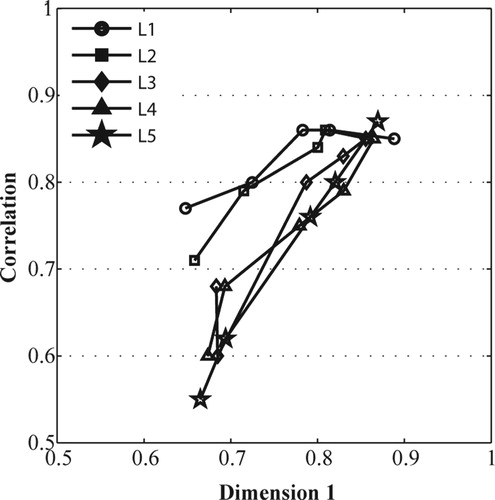
From these results, the correlation between dimension 1 and the graininess parameter was provided by the BYK-mac-i is better (r² = 0.95 vs. r² = 0.89). This result was expected because the graininess value was optimized by a visual experiment. On the contrary, the parameters proposed by the gonio-hyperspectral imaging system were defined by only processing the image. For this reason, the found correlation seemed to guarantee the validity of this system for characterizing such coatings, although it was necessary to combine the correlation parameter with the visual perception to improve the graininess characterization.

Furthermore, the other parameters proposed by the gonio-hyperspectral system were considered to find a relationship with Dimension 2. In this way, the first-order (entropy, energy and asymmetry) and the second-order statistics (contrast, correlation, energy and homogeneity) were compared with Dimension 2. However, it was not possible to define any relationship with this dimension.

For this reason, other attempts were made to find a metrological variable for Dimension 2 based on image processing. Hence the autocorrelation function was computed as it is a good texture descriptor (23). From the autocorrelation function, it is possible to define a texture like a particular signature by calculating the periodicity of the texture, and by computing some parameters associated with this function. In addition, the Fourier transform of images was computed to calculate the distinctiveness, which can be understood as a contrast parameter because it is defined after taking into account the maximum peak value and the minimum surrounding values (23). Nevertheless, no relationship was found with Dimension 2. As the previous results showed a relationship between the graininess effect and the lightness value, it seemed coherent to think that this second dimension was related with the lightness value or with the image contrast. So it was necessary to apply other imaging processes to obtain other parameters related with this attribute to figure out the physical meaning of this dimension. However, the imaging process is a complex topic and goes beyond the scope of this paper. It might can be interesting to establish the visual differences in the graininess of samples with distinct lightness values. That is, the current visual experiment was designed by fixing the lightness value in the samples to be compared. The new experiment should be done by comparing samples with different lightness values. This would allow more information to be found with the interaction between the graininess and the lightness values, while MDS could provide new mathematical dimensions that better correlate with physical or perceptual dimensions.

4. Conclusions

In this work, graininess characterization was conducted by MDS and visual perception. The input data for this algorithm were based on a dissimilarity matrix obtained by a visual experiment. A psychophysical experiment, based on the interval method (point-rating scaling), was designed to establish graininess differences among samples. The samples used belong to the Effect Navigator® chart, composed of 25 samples divided into 5 different groups according to the lightness value. The results from this experiment were used to apply MDS. From this analysis, we conclude that two dimensions are involved in graininess perception.

The multidimensional analysis provides statistical results about the dissimilarities or differences between samples, and a good correlation between the visual differences provided by the designed visual experiment and those obtained by the multidimensional analysis was verified.

Finally, a relationship between the visual and the instrumental graininess was evaluated by taking into account two different instruments. On the one hand, the graininess value (G) provided by the BYK-mac-i instrument was considered. The first dimension perfectly matched the instrumental graininess, while no correlation was found between any variable and the second dimension. On the other hand, the parameters proposed by the gonio-hyperspectral system were considered, and focused on the first- and second-order statistics. A good relationship was found between the first dimensionand the correlation parameter, defined as the digital-level linear dependencies in the image. The other parameters were also considered to confer meaning to the second dimension. However, there was no correlation with any feature associated with the co-occurrence matrix. Therefore, the autocorrelation function and the Fourier transform were obtained to find a parameter that was related to the second dimension, but not successfully. Since no correlation of this second dimension with any measurable quantity was found, future research is needed to look for new information related to it. A possible attempt would be to apply new imaging processes to establish a relationship between the second mathematical dimension and a metrological one. Furthermore, other visual experiments can be designed to better establish or define the mathematical dimensions. Thus, a new visual experiment could be conducted by obtaining visual differences based on graininess, although samples with different lightness should be analysed as well. In this way, the input data for the MDS algorithm would be built after taking into account the interaction or relationship between graininess and lightness, and more useful information could be obtained with the MDS algorithm to better correlate the mathematical and metrological dimensions.

Acknowledgements

The authors thank all volunteer observers who participated in our experiment.

Disclosure statement

No potential conflict of interest was reported by the authors.

Additional information

Funding

The authors are grateful to the EMRP for funding Project ‘Multidimensional Reflectometry for Industry’ (JRPI21) and Project ‘Bidirectional reflectance definitions’ (16NRM08). The EMRP is jointly funded by EMRP participating countries within EURAMET and the European Union. We thank the Spanish Ministry of Economy and Competitiveness for Project DPI2015-65814-R.

References

- Charvat, R.A. Coloring of Plastics: Fundamentals; Society of Plastics Engineers Monographs; Wiley: New York, 2005.
- Debeljak, M.; Hladnik, A.; Černe, L.; Gregor-Svetec, D. Color Res. Appl. 2012, 38 (3), 168–176. doi: 10.1002/col.20753
- Mirhabibi, A.R. Ceramic Coatings for Pigments. In Ceramic Coatings-Applications in Engineering, InTech: Rijeka, 2012; pp 237–258.
- Streitberger, H.-J.; Dossel, K.-F. Automotive Paints and Coatings, John Wiley & Sons: Weinheim, 2008.
- Topp, K.; Haase, H.; Degen, C.; Illing, G.; Mahltig, B. J. Coatings Technol. Res. 2014, 11 (6), 943–957. doi: 10.1007/s11998-014-9605-8
- Klein, G.A.; Meyrath, T. Industrial Color Physics; Springer, 2010; Vol. 154.
- ASTM, E. 284–13b. Standard Terminology of Appearance; ASTM: West Conshohocken, PA, 2010.
- Kirchner, E.J.J.; van den Kieboom, G.J.; Njo, L.; Supèr, R.; Gottenbos, R. Color Res. Appl. 2007, 32 (4), 255–266. doi: 10.1002/col.20328
- McCamy, C.S. Color Res. Appl. 1996, 21 (4), 292–304. doi: 10.1002/(SICI)1520-6378(199608)21:4<292::AID-COL4>3.0.CO;2-L
- McCamy, C.S. Color Res. Appl. 1998, 23 (6), 362–373. doi: 10.1002/(SICI)1520-6378(199812)23:6<362::AID-COL4>3.0.CO;2-5
- Kirchner, E.; Van der Lans, I.; Perales, E.; Martínez-Verdú, F.; Campos, J.; Ferrero, A. J. Opt. Soc. Am. A. Opt. Image. Sci. Vis. 2015, 32 (5), 921–927. doi: 10.1364/JOSAA.32.000921
- BYK-Gardner. BYK-mac-i. https://www.byk.com.
- Gómez, O.; Perales, E.; Chorro, E.; Viqueira, V.; Martínez-Verdú, F.M. Appl. Opt. 2016, 55 (23), 6458–6463. doi: 10.1364/AO.55.006458
- Ferrero, A.; Velázquez, J.L.; Perales, E.; Campos, J.; Martínez Verdú, F.M. Opt. Express 2018, 26 (23), 30116–30127. doi: 10.1364/OE.26.030116
- Bartleson, C.J.; Grum, F.C. Visual Measurements, Academic Press: New York, 1984; Vol. 5.
- Borg, I.; Groenen, P.J.F. Modern Multidimensional Scaling: Theory and Applications, Springer: New York, 2005.
- Borg, I.; Groenen, P.J.F.; Mair, P. Applied Multidimensional Scaling and Unfolding, Springer: Cham, 2017.
- Winston Wang, Z.; Ronnier Luo, M. Color. Technol. 2016, 132, 153–161. doi: 10.1111/cote.12203
- Burgos Fernández, F.J. Gonio-Hyperspectral Imaging System Based on Light-Emitting Diodes for the Analysis of Automotive Coatings, 2016.
- Burgos-Fernández, F.J.; Vilaseca, M.; Perales, E.; Chorro, E.; Martínez-Verdú, F.M.; Fernández-Dorado, J.; Pujol, J. Appl. Opt. 2017, 56 (25), 7194–7203. doi: 10.1364/AO.56.007194
- Gonzalez, R.C.; Woods, R.E.; Eddins, S.L. Digital Image Processing Using MATLAB; Pearson-Prentice-Hall: Upper Saddle River, NJ, 2004; Vol. 624.
- Herrera, J.A.; Vilaseca, M.; Düll, J.; Arjona, M.; Torrecilla, E.; Pujol, J. Color Res. Appl. 2011, 36 (5), 373–382. doi: 10.1002/col.20635
- Maria, P.; Pedro, G.S. Image Processing Dealing with Texture, Wiley: Chichester, 2006.
- Haindl, M.; Filip, J. Visual Texture: Accurate Material Appearance Measurement, Representation and Modeling, Springer: London, 2013.
- Tamura, H.; Mori, S.; Yamawaki, T. IEEE Trans. Syst. Man. Cybern. 1978, 8 (6), 460–473. doi: 10.1109/TSMC.1978.4309999