Factors affecting the measurement resolution of super-resolution techniques based on speckle interferometry

ABSTRACT

A technique is proposed to observe the shape of an object beyond the diffraction limit by analysing the phase of light based on speckle interferometry. Several conditions must be considered during the measurement process to use this technique to observe detailed microstructure. In this study, the primary factors in the measurement process are investigated, and the influence of each factor on the measurement resolution is evaluated. Moreover, the optimum conditions for each factor are proposed. Under appropriate measurement conditions, this measurement technique enables the observation of microstructure beyond the diffraction limit with a high resolution of approximately 100 nm. By proposing proper measurement conditions for this new method of observing beyond the diffraction limit by detecting the phase of light, an environment is created to extend the fields of use including bio-related technologies.

KEYWORDS:

• Super resolution
• proper measurement condition
• speckle interferometry
• phase analysis

1. Introduction

Super-resolution technology is important in bio-related research, wherein microstructure is frequently observed, and there is a demand for the development of technology to observe biological activity [1–3]. However, it is difficult to observe microstructure using optical microscopes because of light diffraction [4]; thus, electron microscopes are generally used [1–3].

Recently, the observation of microstructure using fluorescent proteins has become popular in the field of biotechnology, and new technologies to promote biotechnology research, such as photoactivated localization microscopy (PALM) and stimulated emission depletion (STED), have been developed [5–7]. However, it is difficult to observe the dynamic behaviour of living organisms using such technologies. Thus, optical imaging using an optical camera as an area sensor is indispensable for capturing two-dimensional (2D) images of dynamically active organisms. However, image acquisition beyond the Rayleigh limit proves a challenge because of the diffraction of light, [4,8,9] and 2D observation of microstructures cannot generally be performed using a camera. However, a technique to observe the shape of an object beyond the diffraction limit by analysing the phase of light based on speckle interferometry has recently been proposed [10–14].

In speckle interferometry, deformation measurement with high resolution is realized using speckles to detect the amount of deformation of the measurement object in terms of the amount of change in the phase of the light [15–17].

In the commonly used speckle interferometry, when coherent light such as a laser is scattered on a rough surface, beams of scattered light interfere with each other and pass through the lens aperture, forming a speckle pattern, which is a granular interference pattern that records the phase components of light. The speckle pattern is captured before and after deformation and its phase is detected by calculating a specklegram using these speckle patterns. The change in shape was measured based on the phase distribution [15–18].

In the fringe analysis method used in this study, the speckle pattern is detected using an optical system that produces a speckle pattern without bias components resulting from the use of the off-axis technique, as reported in a previous study, with the objective of achieving an even higher resolution. In addition, a filtering process using the Fourier transform is used to remove noise in the speckle pattern and extract a fringe image containing only the amount of phase change corresponding to the deformation. Subsequently, the phase difference before and after deformation is detected at a high resolution by applying the spatial fringe analysis method to this fringe image [19–22].

Currently, the off-axis technique and filtering technology enable measuring the deformation of rough surfaces with a resolution of approximately 5 nm using only two speckle patterns obtained before and after the deformation. Using the fringe image processing technique of speckle interferometry as a high-resolution phase detection technique, a new technique can be developed to enable the observation of microstructure beyond the diffraction limit [10–14].

In this technique, the optimum conditions for several factors must be established during the measurement process to observe the microstructure in detail. In the developmental stage of this new technology, microstructure was observed by determining the optimal conditions through trial and error in each measurement experiment to capture images that are more suitable for analysis. Therefore, the specific settings required for each factor to enable observation at a high resolution remain unclear.

In this study, the required measurement conditions for the optical system, factors to be considered when capturing images, and conditions that affect the measurement resolution in image processing were investigated, and the optimum setting for each factor to improve the measurement resolution using this method is discussed.

Specifically, the conditions to be considered during measurements were identified and their settings were systematically studied. This clarifies the general conditions for using the proposed technique to observe the shape of objects beyond the diffraction limit by analysing the phase of light based on speckle interferometry [15–18].

Consequently, various measurement conditions required for this new super-resolution technique to serve as a useful method in the observation of microstructure were identified.

2. Measurement principle

2.1. Principle of shape measurement based on speckle interferometry

Using an optical system of speckle interferometry with high phase resolution, three-dimensional shape measurement [15–19] can be performed according to the following measurement principle:

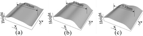
If the cross-section of the object in the x-direction is defined as f(x), as shown in Figure 1(a), and if the object is shifted laterally by exactly δx, then, the new cross-section of the object is f(x + δx), as shown in Figure 1(b).

Figure 1. Principal of analyzing method. (a) Before lateral shift. (b) After lateral shift.

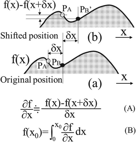
Here, if the deformation f(x) - f(x + δx) resulting from the lateral shift is rigorously analysed using speckle interferometry and the value is divided by the lateral shift to obtain a value corresponding to the approximate derivative of the object shape in the x-direction (∂f/∂x), as shown in Equation (A) of Figure 1.

Furthermore, by integrating this derivative coefficient in the x-direction, f(x) can be estimated, as expressed in Equation (B), and the shape of the measured object can be reconstructed.

Based on this idea, 3D microstructure can be measured beyond the diffraction limit of the objective lens using scattered light as the illumination source [10–14].

2.2. Measurement principle concerning super-resolution

When observing microstructure through the lens of an optical microscope, there is a limit to the confirmation of two points on an object under observation as two independent points using intensity distribution because of the Rayleigh criterion. Therefore, light from the microstructure beyond the diffraction limit cannot be observed as two independent points. Consequently, it was assumed that microstructures beyond the Rayleigh criterion could not be clearly observed [4,8,9].

In this study, two adjacent points on a measured object are not recognized as two independent point images using a single image, but the three-dimensional shape of microstructure beyond the diffraction limit is measured by detecting the phase change in light. This is achieved by physically moving the measurement object several tens of nanometres within the field of view of the lens to obtain two different images [10]. Specifically, if the perfect optical system shown in Figure 2 is set up, even if the light emitted from point P0 on the measured object passes through the lens and is scattered in various directions, a portion of the light always reaches the confocal point P0’ corresponding to point P0 on the surface of the measured object [9].

Figure 2. Detection of two dimensional phase distribution using perfect optical system.

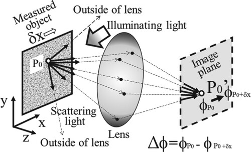
In this case, although a portion of the higher-order diffracted light may be outside of the lens area owing to diffraction phenomena, provided there is scattered light that has passed through the lens, the light is concentrated at the confocal point. Therefore, when a portion of the light from the measured object reaches the confocal point, beams of light that have passed through various optical paths interfere with each other. Owing to this interference phenomenon, each confocal point that spatially corresponds to each measurement point on the measurement object has a phase distribution ϕ_P0 that is related to the optical path length from the measurement point [20].

Furthermore, when a measured object moves several tens of nanometres (δx) in the lateral direction, the phase of each point changes to ϕ_{P0 + δx} based on the amount of the lateral shift. This change occurs with a change in the optical path length from the measured object to the image plane through the lens. Here, when scattered light with ray vectors in multiple directions is used as the illumination source, additional reflected light from the measurement object passes through the lens. Consequently, more light passes through the aperture to form a speckle.

3. Optical system

The speckle interferometer used in this experiment is shown in Figure 3. In this optical system, the beam emitted from a laser (wavelength 671 nm, 100 mW) was split by a polarizing beam splitter while adjusting the intensity of the object and reference lights. The reference light was collimated using a collimator and interfered with the object light at a beam splitter (BS) installed in front of the image sensor to form a speckle pattern with carrier fringes.

Figure 3. Optical system.

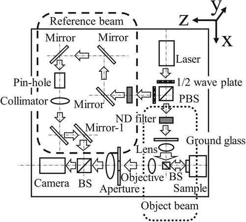
By contrast, the object light was irradiated as illumination source onto the measurement object by collecting it with a lens as scattered light with multidirectional light vectors generated after passing through ground glass. The scattered light reflected on the object surface was focused as scattered light containing phase information by an objective lens (M-Plan Apo 200× manufactured by Mitutoyo Corporation, NA 0.62, magnification 200×). This scattered light containing phase information passes through the pinhole of the imaging lens, as shown in Figure 3, interferes with the reference light at the beam splitter (BS), and then reaches the image sensor (pixel size 1.6 µm, number of pixels 1024 × 1024, grey scale resolution 12 bits). In the experiment, a pinhole was used to control the speckle diameter.

In this case, the diffraction limit was determined to be 660 nm ( =  0.61 × 671/0.62) based on the laser wavelength and numerical aperture (NA) of the objective lens. The optical system is compact (600 mm × 700 mm) with a honeycomb base on an active vibration isolation table (SAT-56: Showa Science Active Vibration Isolation Table) and can be easily used for measurement using mechanical vibration without the need for a special darkroom. The optical system is mounted on a table, as shown in Figure 3.

Subsequently, the specific settings that needed to be established during the measurement and the effect of these settings on the measurement results were investigated.

It is generally known that shortening the wavelength of a light source is effective for obtaining high-resolution optical measurements. However, in this study, the measurement sample was prepared by drawing lines on a resist film fabricated on a silicon wafer with a thickness of 250 nm using an electron beam lithography system. It was assumed that a groove with a depth of 250 nm could be measured. If the step in the optical measurement is 250 nm, the optical path length would be 500 nm, which is double the depth of the groove because the light would make a round trip. Therefore, a light source with a wavelength of 671 nm was used in this experiment to avoid difficulty in measuring the phase change of the light, because the wavelength of 671 nm is not close to the optical path length of 500 nm [10–14].

In addition, because the current camera element is made of silicon, which has a high sensitivity to red light, using 671 nm laser light can yield brighter images. Furthermore, the optical system was composed of optical elements with a design wavelength of approximately 600 nm.

However, in this study, the effect of measurement conditions on the results could not be evaluated using light sources with wavelengths other than 671 nm. It was assumed that the influence of each factor considered in this study would remain the same regardless of the wavelength. Based on the results, the general execution of this method for measurement and analysis is discussed.

However, it is necessary to investigate the effect of light source wavelength in a future study by comparing the results obtained at a wavelength of 671 nm with those obtained using a light source with a shorter wavelength.

4. Fringe analysis method

The fringe analysis method used in this study has been reported previously [18,19,21]. However, as the objective of this study is to discuss the proper conditions for fringe analysis in detail, an overview of the fringe analysis technique is depicted in the flowchart shown in Figure 4, including examples of the processing results in each step. The measurement results for the microstructure shown in Figures 5 and 6 correspond to a groove (SEM image) with a width of 530 nm and depth of 500 nm (Figure 5(a)).

Figure 4. Flow chart of processing.

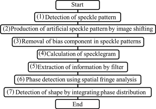
Figure 5. Image processing. (a) SEM image. (b) Speckle pattern. (c) Artificial speckle pattern as second speckle pattern. (d) Speckle pattern in frequency domain. (e) Specklegram. (f) Specklegram in frequency domain. (g) Filtered specklegram.

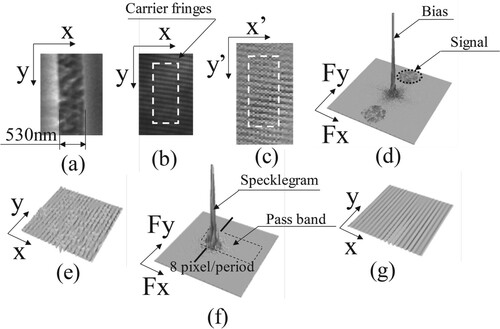
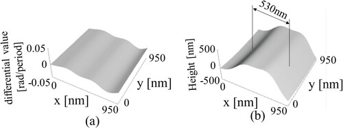
Figure 6. Measured result. (a) Differential distribution of phase. (b) Three dimensional shape.

4.1. Detection of speckle pattern

In the analysis process, represented by step (1) of the flowchart in Figure 4, an image was captured and it was assumed that the area enclosed by the dashed line in Figure 5(b) was the area where the measurement object existed. The image was captured by an off-axis optical system; therefore, carrier fringes exist in the image because of the angles between the wavefronts of the object light and the reference light. However, as the diffraction limit of this optical system is 660 nm, as mentioned previously, the 530 nm groove shown in Figure 5(a) cannot be seen in the image.

The processing performed in this study takes an image beyond the diffraction limit as input, wherein the shape of the object is not visible as a 2D image, and processes it to capture the shape of the object image as a phase distribution. This is an unusual process that takes something invisible and converts it into something visible. To achieve this process, an observable image (visible mark) that can be directly observed as a 2D image and does not exceed the diffraction limit is prepared in advance in the vicinity of the measurement object. The coordinates of this observable image are used as a guide for processing the area where the object that exceeds the diffraction limit is assumed to exist. Using such marks, the aforementioned analysis was achieved by performing the following steps.

4.2. Production of artificial speckle pattern by image shifting

To analyse the time series of the measured object using moving images, an artificial speckle pattern can be generated as a second speckle pattern to measure the shape of the microstructure with only one speckle pattern, without the need to obtain two speckle patterns before and after the physical lateral shift of the speckle pattern. This technique was proposed in a previous study [11].

This process enables capturing the dynamic changes of the measured object in a time series, as it eliminates the need to physically move the object before capturing images.

For this process, an artificial speckle pattern was created, as shown in Figure 5(c), by laterally shifting the speckle pattern captured in step (1) of Figure 4. Figure 5(c) is produced by shifting the speckle pattern shown in Figure 5(b) by three pixels in the x direction.

4.3. Removal of bias component in speckle patterns

The results of the Fourier transform of the captured speckle pattern shown in Figure 5(b) are presented in Figure 5(d). In the optical system shown in Figure 3, the carrier fringes shown in Figure 5(b) are generated because of the angles between the object and reference light wavefronts, resulting in interference fringes between the object light originating from the objective lens and the reference light. This carrier fringe produces a speckle pattern that can be separated from the signal to bias components in the frequency domain when the speckle pattern is Fourier-transformed, as shown in Figure 5(d). Separating the signal component from the bias component in the frequency domain enables the extraction of a speckle pattern without the bias component.

Using these speckle patterns before and after the lateral shift, the deformed carrier fringe image corresponding to the specklegram in general speckle interferometry can be calculated. Specifically, a specklegram including only the phase change Δφ, as indicated by step (4) in Figure 4, can be calculated as the result shown in Figure 5(e). In this specklegram, the carrier fringe image is modulated by the phase change Δφ.

4.4. Extraction of information by filter

The fringe image after processing shown in step (4) of Figure 4 still includes a large amount of speckle noise, as shown in Figure 5(e). Therefore, a filter is used to remove the noise, as indicated by step (5) in Figure 4. In this process, the carrier fringe component of the specklegram was set to 8-pixel cycles in the next phase detection calculation using the spatial fringe analysis method. Therefore, the signal components are distributed in the x-direction in the frequency domain at approximately 8-pixel cycles, as shown in Figure 5(f). If the passband is set in the x-direction from the point of the 8-pixel cycle to an excessively high frequency region, it will be influenced by noise. However, if a narrow passband is set, the cross-sectional shape of the measurement microstructure can no longer be reproduced. In the y-direction, the measured structure is a long groove-like element, as shown in Figure 5(a); therefore, the information is considered to exist as a distribution in the low-frequency domain. Thus, by setting an appropriate passband for the process corresponding to step (5) in Figure 4, a modulated carrier fringe can be extracted, as shown in Figure 5(g), in which the effect of noise is reduced. Evidently, an appropriate setting of the passband in filtering is crucial for achieving a clearer image.

4.5. Phase detection using the spatial fringe analysis method

From the information extracted in step (4), only the amount of phase change can be filtered out, as indicated by step (5) in Figure 4. The phase change due to lateral shifting can be detected with high resolution from the deformed carrier fringe shown in Figure 5(g) using the spatial fringe analysis method, as indicated by step (6) in Figure 4.

4.6. Detection of shape by integrating phase distribution

As the result shown in Figure 6(a) represents the derivative of the shape of the microstructure, the three-dimensional shape shown in Figure 6(b) can be reproduced by integrating with respect to the direction in which the lateral shift was performed, as indicated by step (7) in Figure 4. The direction of lateral shift was discussed in detail in the previous paper [23]. These results demonstrate that a three-dimensional shape can be reproduced using an appropriate setting of the filter (Figure 5(f)) in conjunction with this method [10–14].

Moreover, these results indicate that setting the position of the measurement object as the coordinate in the image in advance enables the correct identification of the groove shape even when the measurement object is beyond the diffraction limit, as shown in Figure 6(b), if microstructure exists in the measurement area.

If there are no structures, such as grooves, in the SEM image, as shown in Figure 7(a), a flat structure, as shown in Figure 7(c), is detected when the image is captured and analysed, as shown in Figure 7(b).

Figure 7. Measured results. (a) SEM image. (b) Speckle pattern. (c) Three dimensional shape.

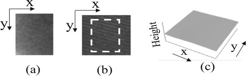
Based on these results, it can be assumed that all cases in which the phase distribution of a groove structure is detected within the measurement area are the result of detecting the shapes of the structures present in the measurement area.

5. Factors affecting measurement resolution and their respective effects on measurement results

5.1. Measurement factors that must be considered

In this study, the brightness of images is related to the signal/noise ratio of measured images, and the out-of-focus magnitude of the imaging device has a large influence on the measurement results, assuming the measurement principle that scattered light emitted from each point on the measurement object in a perfect optical system is captured at a point on the imaging device.

Furthermore, in speckle interferometry, the diameter of the aperture of the imaging optics simultaneously determines the speckle diameter and bandwidth of the spatial information in the speckle; thus, the diameter of the aperture of the imaging optics has a significant effect on the shape of the measurement object.

In addition, because speckles were originally considered to be noise components [24], the specklegram calculated from the speckles before and after the lateral shift contains considerable noise, as shown in Figure 5(e). To remove this noise, it is necessary to use a filter to extract the phase component of the light [22]. The passband of this filter is also considered to affect the measurement results. Another factor that needs to be considered in the optical system is the area of the measurement object covered by a single pixel of the camera. If a single pixel covers a large area, the spatial frequency that each pixel can detect is expected to be low, and if it covers a small area, the spatial frequency is expected to be high. However, in this study, each pixel size of the image device was fixed at 1.6 × 1.6 µm, and the measured area per pixel was set by changing the lens magnification of the optical system during measurement.

Therefore, because the effect of a change in the pixel size of the camera cannot be directly investigated, we measured the effect on the measurement results under the conditions used, including the characteristics of the camera lens.

The results of the study of each factor are presented in the following subsections. However, the effect of the light source wavelength, which was not considered in this study, needs to be further evaluated using a light source with a different wavelength. This is because the lenses of an optical system have wavelength dependency in optical measurements. Therefore, it is necessary to examine this factor, including improvements in the optical system, in the future.

5.2. Effect of image brightness

Figure 8 illustrates the effect of image brightness. Figure 8(b), (c), (d), and (e) show images of a measurement object, and Figure 8(f), (g), (h), and (i) show the results of shape analysis for each value of brightness shown in Figure 8(b), (c), (d), and (e), respectively.

Figure 8. Measured results (Brightness). (a) Brightness distribution in A-A’ cross section. (b),(c),(d),(e) Specklepatterns under each brightness shown in (a) (f),(g),(h),(i) Three dimensional shape under each brightness shown in (a).

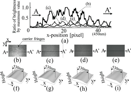
The intensity distribution at cross-section A-A’ in each image is shown in Figure 8(a). The maximum value of the brightest image (Figure 8(b)) was assumed to be 1, and each brightness distribution was considered as a ratio with respect to this value.

In each case, it was confirmed that carrier fringes were used in the process to remove the bias component of the speckle. The periodicity of the brightness is due to the carrier fringes. Although the brightness of the image decreases in Figure 8(b), (c), (d), and (e), the shape measurement results were able to reconstruct the shape, as shown in Figure 8(h) for Figure 8(d). The shape can be reconstructed even for Figure 8(e), as shown in Figure 8(i). Because the phase of the light was analysed, the influence of light intensity on the measurement results was considered to be small.

5.3. Effect of out-of-focus magnitude of the measurement object

The depth of focus of the optical system used in this study was 979.1 nm, or approximately 1 µm, using the expression 0.61 × λ/NA². However, it is challenging to set the measurement object within this range (1 µm). In this measurement system, the measurement object was set on the piezo stage and the position of the object was set to almost coincide with the focal point by changing the input control voltage to the stage.

Figure 9 shows the measurement results when the focal position was varied by ±1 µm by moving the measurement position back and forth. When the measurement target was moved forward by 1 µm from the state shown in Figure 9(b), the height of the shape decreased, as shown in Figure 9(c). Conversely, when it was moved backward by 1 µm, the shape collapsed, as shown in Figure 9(a). By losing focus, the scattered light reflected from each point on the measurement object did not focus on a single point on the image device, and a shape with a high-frequency component, such as the edge-like shape of the measurement object, could not be reconstructed.

Figure 9. Measured result (focus). (a) Below focus (−1µm). (b) Just focus. (c) Over focus (1µm).

Because the measurement technique is based on the measurement principle presented in Figure 2, it is clear that the focusing operation is an important setting. However, focusing on objects beyond the diffraction limit is an extremely difficult process. Thus, phenomena such as the beam waist, wherein the focus of the lens does not necessarily converge to a single point, as well as the problem of perfect optics, are limitations of this measurement principle. In a future study, it will be necessary to investigate the diffraction of airy discs and other materials to determine the resolution of the present method. In this study, large arrows were drawn on the measurement object to mark the vicinity of the object that exceeded the diffraction limit, and the arrows were then focused to determine the measurement position and focus. However, when observing the actual image, an automatic focusing system was necessary based on the results shown in Figure 9.

5.4. Effect of a change in frequency bandwidth based on the aperture diameter of the imaging optics

In speckle interferometry, the speckle diameter is an important measurement factor [22]. For large deformations, the speckles in the speckle pattern before and after deformation must overlap spatially to obtain the phase related to the deformation. Thus, a small aperture diameter of the imaging optics was selected to increase the speckle diameter. However, when the speckle diameter increases, the bandwidth of the speckle information becomes narrower in the frequency domain.

If a deformation measurement is performed under such a condition, the measurement of extremely uneven shapes with high spatial frequency components cannot be performed. Meanwhile, if the speckle diameter is set to a smaller value, the bandwidth of the information recorded in the speckle becomes wider and it becomes possible to measure shapes with severe irregularities. However, as the speckle diameter decreases, the corresponding speckles do not overlap before and after deformation, and the measurement of a large deformation becomes impossible.

Because the process in this study uses a lateral shift of several tens of nanometres without the problem of overlap of measured areas before and after deformation, it is advantageous to set the aperture diameter of the imaging optics as large as possible so that it can handle high-frequency components.

Based on this idea, the results were examined when the aperture diameter of the imaging optical system was set to a large value. However, it must be considered that focusing becomes difficult when the diameter is widened.

The measurement results are shown in Figure 10. Figure 10(a), (b), and (c) show the measurement results when the aperture (F-number) of the imaging lens was changed to f = 8, 11, and 16, respectively. Figure 10(d), (e), and (f) show the distribution of information in the frequency domain when the speckle patterns captured under the condition of each aperture were Fourier-transformed. It can be seen that by narrowing the aperture from f = 8 to f = 16, the bandwidth became narrower.

Figure 10. Measured result (frequency range of optical system). (a)Three dimensional shape (f = 8). (b) Three dimensional shape (f = 11). (c) Three dimensional shape (f = 16). (d) Speckle pattern in frequency domain (f = 8). (e) Speckle pattern in frequency domain (f = 11). (f) Speckle pattern in frequency domain (f = 16). (g) Shape in B-B’ cross section.

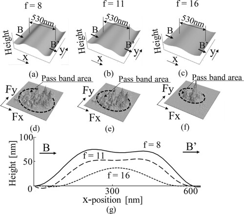
As a result, cross sections B-B’ of the shapes in Figures 10(a), (b), and (c) are clearly smooth with the missing high-frequency components, as shown in Figure 10(g).

The result of this verification is consistent with the basic properties of speckle interferometry.

When observing microstructure using this method, it is desirable to increase the aperture width if the focusing problem is eliminated.

5.5. Effect of filter passband for noise reduction in specklegrams

Information on the phase of light from specklegrams caused by a lateral shift of the object, as shown in Figure 5(e), was extracted using the spatial fringe analysis method [18,19]. In this process, the specklegram in Figure 5(e) was Fourier transformed, as shown in Figure 5(f), and the result shown in Figure 5(g) was denoised through a filtering process by setting the passband in the frequency domain. In this case, the change in the filter passband was considered to have a strong influence on the measurement results, as discussed in Section 5.4.

As shown in Figure 11, to perform the spatial fringe analysis for a specklegram with a fundamental carrier frequency of 8 pixels per cycle, the passband was set (a) from 8 to 7, (b) 8–5.5, (c) 8–4.5, (d) 8–3.7, and (e) 8–3.1 pixels per cycle at points A, B, C, D, and E, respectively. As the passband was expanded in the direction of higher frequencies to points C, D, and E, the measurement results clearly show the shape of the measured grooves.

Figure 11. Measured result (Passband of filter). (a) 8–7 pixel/period (from O to A). (b) 8-5.5 pixel/period (from O to B). (c) 8-4.5 pixel/period (from O to C). (d) 8-3.7 pixel/period (from O to D). (e) 8-3.1 pixel/period (from O to E).

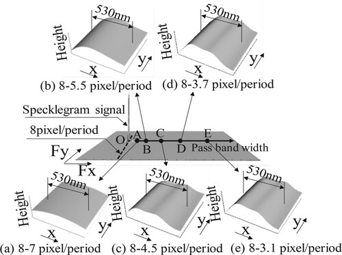
It can be seen that passing signals with a frequency component as high as possible is an important factor for obtaining a more accurate shape of a measurement object. Meanwhile, setting of the filter passband must be tailored to the situation because a wider bandwidth may introduce noise components.

5.6. Influence of the size of the area on a measurement object per pixel of the image element

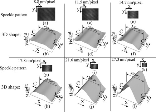
The size of the area of a measured object corresponding to one pixel of the image element is considered to be an important factor related to spatial resolution. A camera with a pixel pitch of 1.6 µm was used in this optical system, and because the magnification of the objective lens was 200×, one pixel could be set to approximately 8 nm (1600 nm/200 = 8 nm). However, when the actual size of one pixel was set to approximately 8 nm, the captured image of one pixel became dark because of the relationship with the output of the laser light source in this optical system. Therefore, the area corresponding to one pixel was set so that it did not become dark. In this study, the case where the pixel size was varied from 8.8–27.3 nm, was examined. As shown in Figure 12(e), when the pixel size was set to 14.7 nm, a groove shape similar to that of the correctly focused result shown in Figure 9(b) could be observed. Therefore, the condition of 14.7 nm was assumed to be the optimum value for this factor.

Figure 12. Measured result (Length of one pixel on each image). (a) Specklepattern (8.8 nm/pixel), (c) Specklepattern (11.5 nm/pixel), (e) Specklepattern (14.7 nm/pixel), (g) Specklepattern (17.8 nm/pixel), (i) Specklepattern (21.6 nm/pixel), (k) Specklepattern (27.3 nm/pixel). (b) Three dimensional shape (8.8 nm/pixel), (d) Three dimensional shape (11.5 nm/pixel), (f) Three dimensional shape (14.7 nm/pixel), (h) Three dimensional shape (17.8 nm/pixel), (j) Three dimensional shape (21.6 nm/pixel), (l) Three dimensional shape (27.3 nm/pixel).

When observing spatially fine structure, it is considered to be a good strategy to observe as much as possible of a narrow area with one pixel.

However, in this experiment, it was found that good results were not necessarily obtained considering two factors, even if the pixel size was set to that of a narrow area.

One factor is that the size of the image element used in this experiment was set to 1.6 µm, and to change the measured area per pixel without using image elements of other sizes, the corresponding area per pixel was changed by projecting the object magnified by the lens system onto the image element. Therefore, the result was not simply a change in the area size observed through a single image element but the magnification effect of the lens system, and the result included the lens characteristics.

Another important factor in the experiment was the problem of accurately setting the focus of each image while setting the pixel area. As mentioned previously, focusing has a significant influence on the results, and although the measured object was focused using visual focusing marks whenever possible, the results presented in Figure 12 may not necessarily be the result of the same focus setting.

Initially, it was thought that the most appropriate shape would be obtained when the pixel size was set to 8.8 nm; but in fact, a good result was obtained when the pixel size was set to 14.7 nm, resulting in a clear observation of the groove shape of the measurement object.

Figure 13 shows the results of the comparison obtained by aligning the initial point Py shown in Figure 13 with the integration calculation of each cross-section C-C’ in Figure 12.

Figure 13. Measured result (Length of one pixel on each image) on C-C’ cross section in Figure 12.

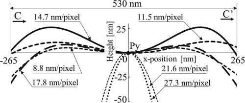
At this initial point, the initial value was set to zero when calculating the 2D shape in the final stage to obtain the shape. When the pixel size was set to 14.7 nm, the cross section exhibited a large undulation.

In contrast, when the pixel size was narrowed to 11.5 or 8.8 nm, the shape became flat and the groove structure of the microstructure became clear. However, at 17.8 nm/pixel (a setting larger than 14.7 nm/pixel), the shape was flat again, similar to the shape observed at 8.8 nm/pixel. This indicates that the clearest shape was not necessarily detected at 8.8 nm/pixel. Therefore, in this experiment, the condition of 14.7 nm/pixel, which observed the shape most clearly, was considered as the best condition for detecting the groove shape.

Furthermore, when the pixel size was further expanded to 21.6 and 27.3 nm/pixel, the results were clearly different from those for 14.7 nm/pixel. These results were considered to be based on the information obtained from the area observed in the measurement; however, the results only confirmed the existence of thin lines rather than a groove structure. This indicates that the measurement results were affected by the setting conditions of the area per pixel. In terms of focus, the setting of the spatial resolution per pixel of the measurement is also an important factor in improving the resolution of the measurement results.

6. Observation of finer structure under proper measurement conditions considering the influence on the measurement results

In the previous section, five factors that affected the measurement results were discussed. Based on these results, the effectiveness of this method in observing finer structures was investigated.

For this purpose, the following conditions were considered: 1) The image should be bright in terms of the signal-to-noise ratio, even if it is not strongly affected by the brightness of the image; 2) In terms of focus, which strongly affects the image, the measured object should be focused as much as possible by preparing and using focusing markers near the measurement object that do not exceed the diffraction limit; 3) Regarding the influence of the frequency passband based on the aperture diameter of the imaging optical system, the aperture diameter should be as large as the optical system allows, and processing should be performed using information from a wider frequency passband; 4) Regarding the effect of the filter passband when removing noise from specklegrams, the passband should be set as wide as possible while considering the amount of noise; 5) Regarding the effect of the pixel size, it is necessary to make the area per pixel as narrow as possible; however, it is important to note that narrowing the area per pixel in this optical system results in the measurement object being enlarged by the lens. In this optical system, lowering the pixel size is not necessarily considered a good condition for including other effects of the optical system because enlargement of the object by the lens needs to be considered. Therefore, in this experiment, the measurement was performed at 14.7 nm/pixel.

Based on the aforementioned conditions, grooves with line widths of 220, 150, 115, and 60 nm (all measured from SEM images) were observed using this method. Because all of them were beyond the diffraction limit of this optical system, it was not possible to observe the shape of each object using the normal optical method. Therefore, the measurement object was observed beforehand using SEM, a map of the distribution of the measurement sample was produced, and the coordinates of the map were used to measure the samples with four different groove widths. The results are shown in Figure 14. It was also initially confirmed that when there was no groove on the map of the measurement object, the measurement result was flat, as shown in Figure 7.

Figure 14. Measured result (Line width). (a) SEM image (220 nm), (d) SEM image (150 nm), (g) SEM image (115 nm), (j) SEM image (60 nm). (b) Speckle pattern (220 nm), (e) Speckle pattern(150 nm), (h) Speckle pattern (115 nm), (k) Speckle pattern (60 nm), (c) Three dimensional shape (220 nm), (f) Three dimensional shape (150 nm), (i) Three dimensional shape (115 nm), (l) Three dimensional shape (60 nm).

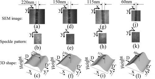
For the four grooves observed in the SEM images in Figure 14(a), (d), (g), and (j), speckle patterns with carrier fringes were captured, as shown in Figure 14(b), (e), (h), and (k), respectively. The shape of the grooves was observed by detecting the phase of the light. Figure 14(c), (f), (i), and (l) show the measurement results. A groove shape is observed in all cases.

The cross-section D-D’ of each measured shape was compared by aligning the initial point Pz shown in Figure 15 with the integration calculation of each cross-section in Figure 14, where the initial value was set to zero, with each cross-section D-D’ displayed in the same way as in Figure 13.

Figure 15. Measured results (Line width) on D-D’ cross section in Figure 14.

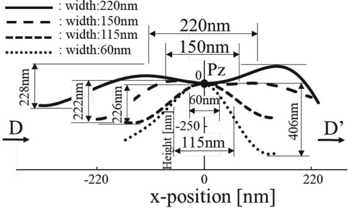
Figure 15 shows the cross-sectional shapes. The three-dimensional shapes of all cross-sections were measured, and the measured line widths were found to be much larger than those of the original structures.

In particular, the measurement result for the groove with a line width of 220 nm showed a wide spread. The groove depth was 228 nm. For line widths of 220, 150, and 115 nm, the groove widths were wider, but the groove depths (approximately 250 nm) were sufficiently deep to be observed, as the grooves were drawn on a 250-nm-thick resist on a silicon wafer as the object. However, for the groove with a width of 60 nm, the depth was 406 nm, which clearly shows that the depth information indicated by the measurement was incorrect. This phenomenon is very similar to the measurement results obtained when the area per pixel was very large for the original linewidth of the object, as shown in Figure 12(j) and (l), where the depth could not be detected correctly.

In any case, this method can detect the existence of structures on a measurement object. In the future, an investigation of the spatial resolution limit of measurements using finer measurement samples under appropriate conditions should be performed.

7. Conclusion

A technique was developed to observe the shape of objects beyond the diffraction limit by analysing the light phase based on speckle interferometry. To use this technique to observe microstructure in detail, several conditions must be considered during the measurement process.

In this study, appropriate conditions and their effects on the measurement results were investigated.

For measurements using this method, the following desirable conditions need to be considered:

1. Regarding the effect of image brightness, although the measurement result is not strongly affected by the brightness of the speckle pattern, it is desirable that the image is bright in terms of the signal-to-noise ratio.

2. Regarding the effect of the out-of-focus magnitude of the measurement object, it is desirable to focus on the image as much as possible, as it strongly affects the results.

3. Regarding the influence of the frequency passband based on the aperture of the imaging optical system, the aperture should be set to a large value, and processing should be performed using information from a wider frequency passband.

4. Regarding the effect of the filter passband in removing noise from specklegrams, it is necessary to set the passband as wide as possible while considering noise removal.

5. Regarding the effect of the pixel size, it is necessary to make the area per pixel as small as possible without using the magnifying effect of the optical system.

6. After setting the conditions considered appropriate for observations in this method, grooves with line widths of 220, 150, 115, and 60 nm were observed. All objects were beyond the diffraction limit, and could not be observed using the traditional method. Although the measured groove widths were wider than the original widths, it was confirmed that the measurement object could be observed using this method. However, in the case of thin-line measurements with high aspect ratios, the measured results exceeded the original depth. In the future, it is necessary to thoroughly investigate the cause of this phenomenon.

In this study, an environment was created to extend the fields of use including bio-related technologies by proposing proper measurement conditions for a novel method that enables observation of objects beyond the diffraction limit by detecting the phase of light.

Disclosure statement

No potential conflict of interest was reported by the author(s).

Additional information

Funding

This work was supported by JSPS KAKENHI [grant no 20H02165].

References

- Garini Y, Vermolen BJ, Young IT. From micro to nano: recent advances in high-resolution microscopy. Curr Opin Biotechnol. 2005;16:3–12.
- Heintzman R, Ficz G. Breaking the resolution limit in light microscopy. Briefings Funct Genomics Proteomics. 2006;5:289–301.
- Huang B. Super-resolution optical microscopy: multiple choices. Curr Opin Chem Biol. 2010;14:10–14.
- Kohler H. On abbe’s theory of image formation in the microscope. Optica Acta: Int J Opt. 1981;28:1691–1701.
- Rust JM, Bate MS, Zhuang X. Sub-diffraction-limit imaging by stochastic optical reconstruction microscopy (STORM). Nat Methods. 2006;3:793–796.
- Betzig E, Patterson HG, Sougrat R, et al. Imaging intracellular fluorescent proteins at nanometer resolution. Science. 2006;313:1642–1645.
- Hell WS, Wichmann J. Breaking the diffraction resolution limit by stimulated emission: stimulated-emission-depletion fluorescence microscopy. Opt Lett. 1994;19:780–782.
- Feynman PR. The Feynman lectures on physics. Reading (MA): Addison-Wesley Publishing Co.; 1989; Chapter 30-3.
- Born M, Wolf E. Principles of optics. 7th ed. New York(NY): Cambridge University press; 1999; p. 199-201 and p. 461-476.
- Arai Y. Three-dimensional shape measurement beyond the diffraction limit of lens using speckle interferometry. J Mod Opt. 2018;65:1866–1874. doi:https://doi.org/10.1080/09500340.2018.1470266.
- Arai Y. Springer proceedings in physics. Springer Proc Phys. 2019;233:1–10. doi:https://doi.org/10.1007/978-981-32-9632-9_1.
- Arai Y. Precise wide-range three-dimensional shape measurement method to measure superfine structures based on speckle interferometry. Opt Eng. 2020;59; doi:https://doi.org/10.1117/1.OE.59.1.014108.
- Arai Y. Consideration of existence of phase information of object shape in zeroth-order diffraction beam using electromagnetic simulation with aperture in front of objective. J Mod Opt. 2020;67:523–530. doi:https://doi.org/10.1080/09500340.2020.1760383.
- Arai Y. Observation of micro-characters using three-dimensional shape measurement method based on speckle interferometry. J Mod Opt. 2020;67:1451–1461. doi:https://doi.org/10.1080/09500340.2020.1864041.
- Sirohi SR. Speckle metrology. New York (NY): Marcel Dekker; 1993; p. 99-234.
- Cloud G. Optical Methods of Engineering analysis. New York(NY): Cambridge University Press; 1995; p. 395-476.
- Malacara D. Optical Shop Testing. New York (NY): John Wiley & Sons; 1992.
- Arai Y, Yokozeki S. Improvement of measuring accuracy of spatial fringe analysis method using a kalman filter and its application. Opt Eng. 2001;40:2605–2611.
- Arai Y. Electronic speckle pattern interferometry based on spatial information using only two sheets of speckle patterns. J Mod Opt. 2014;61:297–306.
- Arai Y. Microshape measurement method using speckle interferometry based on phase analysis. Photonics. 2021;8; doi:https://doi.org/10.3390/photonics8040112.
- Arai Y, Shimamura R, Yokozeki S. Dynamic out-of-plane deformation measurement using virtual speckle patterns. Opt Lasers Eng. 2009;47:563–569.
- Arai Y. Pre-treatment for preventing degradation of measurement accuracy from speckle noise in speckle interferometry. Measurement (Mahwah N J). 2019;136:36–41.
- Arai Y. Shape measurement method of two-dimensional micro-structures beyond the diffraction limit based on speckle interferometry. Photonics. 2021;8:420, doi:https://doi.org/10.3390/photonics8100420.
- George N, Jain A. Speckle reduction using multiple tones of illumination. Appl Opt. 1973;12:1202–1212.