Design performance optimization of laser beam welded joints made for vehicle chassis application using deep neural network-based Krill Herd method

Abstract

The welding to be performed must be defect free, offer lower residual stress and strain, be compact in size and withstand different load conditions. However, the existing investigations in this scenario are still not modernized. Therefore, in this study, a specific welding method called laser beam welding (LBW) is performed and different weld parameters have been inspected and analysed. Advanced instruments based on the non-destructive (ND) are implemented to find the variable LBW responses such as weld bead defects, residuals and strain. The experimentation has been designed using Design Expert software, response surface methodology (RSM) and Box Behnken design (BBD) and verified by analysis of variance (ANOVA) analysis and FIT statistics. Moreover, a hybrid deep neural network-based Krill Herd optimization (DNN-KHO) is implemented to predict the output parameters like, undercut (µm), overlap (µm), total strain (mm/mm) and residual stress (MPa) during welding. The proposed DNN-KHO was also used to optimize LBW input parameters such as, peak power (W), weld speed (mm/s), gas flow rate (l/min) and beam diameter (µm) simultaneously. Predictions show that the proposed DNN-KHO algorithm outperformed by 21.53%, 45.428% and 41.31% higher in accuracy compared to respective hybrid random forest based grey wolf method (RF-GWO), RF and DNN predictions.

Keywords:

• Laser beam welding
• response surface methodology
• ANOVA
• Krill Herd algorithm
• deep neural network

1. Introduction

Residual stresses are the stresses built within a material during manufacturing process or the secondary process such as heat treatment, machining processes or especially the welding operations [1,2]. Hence, the researchers are still looking to solve the issues caused by residual stress formation during manufacturing. The major issues caused by residual stress are dimensional instability, poor durability and fatigue life of the end product/components. Since, welding is widely used high temperature machining process in automobile and construction industries, the researchers are attracted more towards to select and resolve suitable welding processes and fatigue stress buildup during welding. Besides, the welding process and process parameters should be carefully chosen when there is not much residual formation or a high rate of durability to be achieved. Tankova et al. [3] analysed the residual stress formation and behaviour of I section steel members due to the welding operation. The authors implemented a new sectioning method to study and measure residual stresses developed within the sections. Another author, Derakhshan et al. [4] stated welding is a major joining method because welding is easy to handle, efficient, economically viable and productive. Due to heat rise during welding, this process introduces distortion and residuals within the welded materials. Nevertheless, different welding processes must be performed and welded material surfaces are compared using a microscope for study the defects in weld bead geometry. So that, the formation of residual stresses during welding process can be minimized. An X-ray diffractometer (XRD) is another method to determine developed residuals in the welded region. In this regards, Yu and Kim [5] investigated welds’ porosity on zinc coated steel members by analysing the welding process with scanning electron microscopic (SEM) images captured by high resolution cameras. The author concluded the welding current and torch positions significantly affect the formation of porosity. Another author, Ozerov et al. [6], studied the micro hardness and weld pores of the titanium metal matrix composite using SEM and XRD methods. The results evident that the weld made by laser beam welding (LBW) method at ambient conditions produced micropores between 200 µm and 300 µm with improved hardness properties at the micro level.

Being automotive industry is one where the welding process is widely used, the residual stress and defects caused by welding have an effect on the automotive chassis strength. Therefore, feasible weld methods and parameters are carefully selected to avoid residual stresses and defects in weld bead geometry. Svensson et al. [7] found weight reduction in heavy truck chassis, which was essential for trucks to save fuel and achieve extended load carrying capacity. The study showed that weight reduction in heavy truck chassis can be achieved with the use of different welding techniques, different chassis materials and filler materials. Moaaz and Ghazaly [8] mentioned the fatigue life, stress distribution, payload capacity and weight are the most important terms while designing and evaluating of truck chassis members. More attention should be given to flexibility and strength rather than rigidity during the design of truck chassis members. Chen et al. [9] conducted experiments using MAG weld joints on chassis members. The relationship between various input and output parameters of the welding process was analysed. From that study, the authors found possible solutions for the difficulties in measuring the quality of chassis weld joints. On the other hand, the microstructure and strength of the weld bead are the crucial factors for welding process and are mainly influenced by the residual stress developed during welding [10]. The residual stress of the weld bead could be within the favourable limit during LBW, because LBW used less heat input for melting and jointing the metal pieces instead of using huge concentration of uneven heat input [11,12]. In this regard, the researchers tested different LBW processes and various LBW parameters such as welding speed, penetration, width, etc. Most of the studies showed that the laser power was a major influencing process parameter on laser weld defect such as reinforcement (overlap), undercut, etc. Some researchers also gave special attention to detect residual stress development during LBW process. Franco et al. [13] investigated the depth of penetration, weld bead width, weld speed and laser power of LBW module on SS specimens. The result showed that the heat transfer during LBW process was a major parameter that greatly impacts weld joints. Wits and Becker [14] studied the laser beam welded specimens made on additive manufactured titanium (AMT) and conventionally manufactured titanium (CMT). The author achieved air-tight welding on the AMT component with adjusted LBW parameters.

Similarly, the optimal input LBW conditions for a thin inconel sheet were suggested by Jelokhani-Niaraki et al. [15]. The author used response surface methodology (RSM) approach to optimize LBW parameters and identify the relationship between LBW input and output parameters. As a result, the microhardness of welded material was found to be decreasing whenever the input parameters were increased. Whereas, Satyanarayana et al. [16] analysed LBW process parameters using computational fluid dynamics and Taguchi optimization methods. The authors obtained maximum weld depth and minimum HAZ width by manipulating the input parameters with the help of the Taguchi method. Similarly, several authors used RSM, Box Behnken design (BBD), to design LBW experimentation. Apart from BBD, central composite design (CCD) is also another modelling method, which can be developed using RSM [17]. According to the literature, the RSM inbuilt features like analysis of variance (ANOVA) analysis and FIT statistics are suitable to manipulate, validate and modify the derived mathematical model to become more feasible or fit to the actual experimentation, so that the errors can be eliminated or minimized [18,19]. On the other hand, pulsed Nd:YAG LBW process parameters were also optimized by Torabi and Kolahan [20] using RSM methodology and simulated annealing techniques. Results show that the RSM outcomes and the simulated annealing outcomes have good agreement with experimental results.

Besides, several researchers solved optimization problems by implementing machine learning, artificial neural networks, deep neural networks (DNNs) and artificial intelligence (AI) [21–24]. However, the application of hybrid deep neural network-based Krill Herd optimization (DNN-KHO) technique for optimize LBW parameters was not yet discussed by existing researchers. Hence, this study attempts to use a novel DNN-KHO for optimizing LBW parameters to fabricate low weight-high strength vehicle chassis. To support the novelty of the study, the LBW parameters are carefully chosen in order to solve residual stress and strain development during welding because the vehicle chassis members are highly vulnerable to various forces if they are not perfectly welded. Also, the formation of residual stresses during the manufacturing of steel structures may introduce unnecessary deformation, which is difficult to reduce.

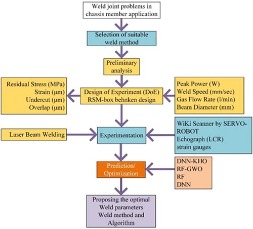
However, many articles discussed on parameters related to weld bead geometry, the research on weld bead defects, such as overlap and undercut, are not sufficient to identify optimum LBW parameters. This leads to identify suitable weld joint type and optimum LBW parameters for vehicle chassis to avoid failures in chassis member weld joints in this study. The material selection, specimen preparation, LBW equipment details and other adapted materials and methods during this study are explained in Section 2. The study was designed using RSM-BBD and experimental results are predicted by using a novel hybrid machine learning technique as given in Section 3. The outcome of this study is discussed, and finally, results are concluded in Sections 4 and 5, respectively. An overview of the proposed study is also presented in Figure 1.

Figure 1. Proposed methodology.

2. Materials and methods

2.1. Selection of material

The existing investigation uses the ASTM A710 grade A steel due to its higher tensile yield strength and tensile ultimate strength properties. However, considering the price and availability of such steel in the market, the present investigation proposes using ASTM A302 alloy steel. ASTM A710 grade A steel and ASTM A302 alloy steel have highly competitive physical, mechanical and thermal behaviours. The physical properties of ASTM A302 alloy steel (as per the manufacturer) are listed in Table 1 [25]. Whereas Table 2 shows the thermal properties of ASTM A302 alloy steel.

Table 1. Physical properties of ASTM A302 alloy steel.

Name of material	ASTM A302 alloy steel
Density (g/cm^3)	7.8
Poisson’s ratio	0.27–0.30
Modulus of elasticity (GPa)	190
Tensile ultimate strength (MPa)	620
Tensile yield strength (MPa)	320
Elongation at 6–50 mm (%)	18
Elongation at 50–200 mm (%)	15

Table 2. Thermal properties of ASTM A302 alloy steel.

Latent heat of fusion (J/g)	Melting completion	Melting onset	Specific heat capacity	Thermal conductivity	Thermal expansion
250	1460 °C	1420 °C	470 J/kg-K	51 W/m-K	13 µm/m-K

Moreover, the ASTM A302 alloy steels are classified into four groups from grade A to grade D based on the percentage of chemical composition. In this study, ASTM A302 grade B alloy steel is used due to its wider applications in automobile chassis frame construction where welding is a major process to complete frame structure [25]. The chemical composition of ASTM A302 alloy steel (as per manufacturer) is listed in Table 3.

Table 3. Chemical composition of ASTM A302 alloy steel (grade B).

C	Mn	P	S	Si	Mo	Fe
0.20–0.25	1.07–1.62	0.035	0.035	0.13–0.45	0.41–0.64	Remaining

2.2. Preparation of specimens

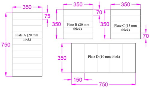
ASTM A302 alloy steel plates having 20 mm, 15 mm and 10 mm are bought. The plates are cut into pieces using 1 kW ‘Sahajanand Brahmastra Infinity 2D Fibre Laser Cutting Machine’ laser cutting machine, which is integrated with a controlling software as shown in Figure 2. The workpieces are cut out from various alloy steel plates namely plate A, plate B, plate C and plate D of different dimensions as shown in Figure 3. According to Figure 3, 10 workpieces, each having a width of 75 mm were cut from plate A, which is 20 mm thick and 750 mm long. Whereas, plate B and plate C that have a length of 350 mm, are to be cut into five pieces each, will have a width of 70 mm. On the other hand, 10 mm thick plate (plate D), which has the dimensions of 750 mm × 350 mm, has to be cut into five pieces, each having a width of 150 mm.

Figure 2. Fibre laser cutting process of workpiece.

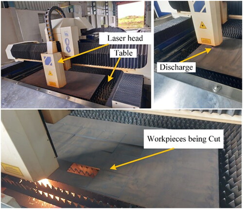
Figure 3. Dimensions of 20 mm, 15 mm and 10 mm thick plates to be cut.

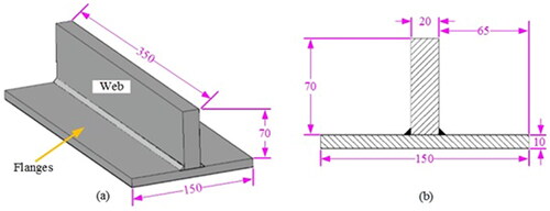
Figure 4(a,b) shows the assembled and two-dimensional view of ‘I’ section to be created after welding. The ‘I’ section is made using two flats (flanges) having dimensions 75 mm × 20 mm × 350 mm, whereas the middle vertical piece (web) has the dimension of 70 mm × 15 mm × 350 mm. Similarly, Figure 5(a,b) shows the assembled view and two-dimensional view of ‘T’ joint after welding. The ‘T’ joint is made of a flat piece (flange) having the dimension of 150 mm × 10 mm × 350 mm and the vertical piece (web) having the dimension of 70 mm × 20 mm × 350 mm.

Figure 4. ‘I’ section with four Butt joints: (a) assembled view and (b) 2D view.

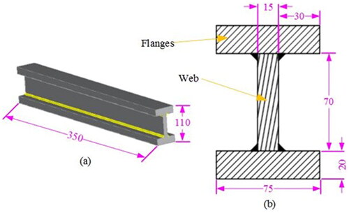
Figure 5. ‘T’ section with two Butt joints: (a) assembled view and (b) 2D view.

2.3. Laser beam welding set-up

The various parts involved in the LBW are a FLASH tube, surrounding lasing material, focusing lens, laser head, gas tank, gas control valves and the gas nozzle and controls. The gas tank contains highly flammable gas. For instance, the present investigation uses argon gas as a shielding gas. The argon gas is a colourless, odourless gas with the same solubility in the water as oxygen. Table 4 shows the properties of argon gas used in the present investigation (as per the seller). The argon (Ar) gas flow rate varies between 8 and 12 l/min in the present investigation to study the rate of a chance of other LBW parameters.

Table 4. Argon gas properties.

Atomic mass	Melting point	Boiling point	Density	CAS number
39.948 g.mol^–1	−189 °C	−185.7 °C	0.00163 g/cm^3	7440-31-1

The LBW welding experiment has been performed using a PB series YAG type laser welding machine. Table 5 shows the different specifications (per the manufacturer) of the HAN*S LASER PB300 series LBW machine used in the present investigation. The cut pieces are fixed on the work table of the automatic welding machine using fixtures or rotating chucks. The gas flow rate, laser head feed rate (welding speed) and beam diameter are pre-set using the LBW controller. During the preliminary analysis, up to five experimentations were conducted using YAG type LBW machine (Figure 6).

Figure 6. YAG type laser beam welding machine PB series.

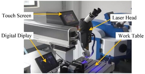
Table 5. HAN*S LASER PB300 manufacturer specifications and features.

Model	Type	Peak power	Pulse width	Positioning method	Cooling type	Input power
PB300	YAG	6–12 kW	0–50	CCD	Water cooled	380 V, 50/60 Hz

2.4. Laser beam welding process parameters

In order to study the residual, strain and weld quality involved in LBW joints, the input parameters such as peak power (W), weld speed (mm/s), gas flow rate (l/min) and beam diameter (mm) are adjusted between 1300–1400 W, 25–35 mm/s, 8–12 l/min and 1–2 mm, respectively (the range of LBW parameters is chosen based on pre-experimentation and literature [15,16,20,21]). Table 6 shows the laser beam weld parameters even more clearly.

Table 6. Range of input parameters.

Peak power (W)	Weld speed (mm/s)	Gas flow rate (l/min)	Beam diameter (mm)
1300	25	8	1
1350	30	10	1.5
1400	35	12	2

2.5. Bead width and strain measurements

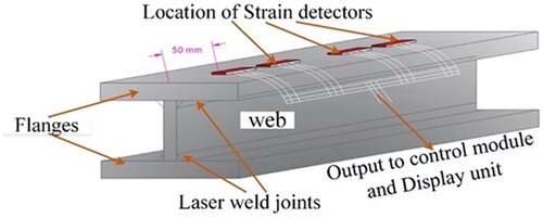
The weld bead geometry, such as bead width, including defects reinforcement (overlap) and undercut, are measured using the Wiki Scan instrument made by Servo-Robot Inc. (Saint-Bruno-de-Montarville, Canada). The Wiki Scan is the most advanced device capable of inspecting weld bead defects reinforcement and overlap (reinforcement) with higher accuracy. The Wiki Scanner works based on the principle of laser beam sensing technology, where the deviations in the reflected laser beams are interpreted and displayed as numbers. The Wiki Scanner inspection device used for weld bead error is shown in Figure 7(a), whereas Figure 7(b) shows the strain detector attachment to the specimen to measure the strain. A couple of strain detectors have been attached to both edges of the beam at a distance of 50 mm from the edge, as shown in Figure 8. As well as, the surface where the detectors are to be fixed is cleaned perfectly to make a tight connection between the specimen and the detectors, this practice will prevent the rise of measurement errors. The prepared specimens are then loaded into a universal testing machine, and the corresponding strain values are noted to the applied unit load.

Figure 7. Weld bead geometry and strain measurements: (a) Wiki Scanner inspection device and (b) strain detector attachment to the workpiece.

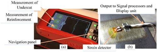
Figure 8. Location of strain gauges.

2.6. Measuring residual stress

Non-destructive (ND) tests are conducted to find the residual stresses formed within the ASTM A302 alloy steel. The ASTM A302 alloy steel material has to be tested before the LBW process and after the LBW process in order to find the residuals formed within the material structure. A universal testing machine and an L_cr device (echograph) made of an acoustic transducer are used. The acoustic transducer works based on the principle of ‘acoustoelasticity’, where the residual stresses formed in the material are measured according to the speed of returning ultrasonic signals from the ASTM A302 alloy steel specimens. According to ‘acoustoelasticity’, the velocity of the ultrasonic signal emitted from the attached L_cr transducer device may vary when it arrives at the collector to the residuals present within the ASTM 302 alloy steel specimens [26,27]. (1) $$\sigma =Eϵ$$(1) where σ is the stress, E is the modulus of elasticity and ε is the strain.

The equation can be rewritten as follows, considering the anharmonic properties of residual stresses, where C is the anharmonic constant. (2) $$\sigma =ϵ(E+C\epsilon )$$(2) (3) $$B=(t-t_o)/\sigma$$(3) (4) $$\sigma =\Delta t/B$$(4)

From Equation (3)(3) $$B=(t-t_o)/\sigma$$(3) , t is the ultrasonic transmission time of LBW welded specimens. t_o is the ultrasonic transmission time when the ASTM A302 alloy steel specimens are at their free state (before LBW). B is the ‘acoustoelasticity’ constant. σ is the $\text{uniaxial or residual stress}.$

The residual formation ($\sigma$) in the LBW welded specimens can be easily calculated by dividing the change in ultrasonic transmission time ($\Delta t$) with B.

3. Design of experiment (DoE) and optimization method

3.1. Response surface methodology

The experimentation has been modelled using the RSM based on BBD. The RSM was developed in the 1950s to predict the optimal conditions in a process in the chemical industry [28]. It consists of statistical techniques based on mathematical methods to develop the relationship between a problem’s factors (input parameters) and responses (output parameters). This relation can be approximated using an LDP model [29,30]. (5) $$y=f^{\prime }\left(x\right)\beta +\epsilon$$(5) where x = (x1 + x2 + x3 + x4……$x_l$)′, f(x)=vector function and ε is the experimental error.

There are two models, called the first-degree model and the second-degree model, that are normally used in the RSM. (6) $$y={\beta }_o+\sum _{i=1}^k{\beta }_i{x}_i+\epsilon$$(6) (7) $$y={\beta }_o+\sum _{i=1}^k{\beta }_i{x}_i+{\sum }_{i<j}\sum {\beta }_{ij}{x}_i{x}_j+\sum _{i=1}^k{\beta }_{ii}{x}_i^2+\epsilon$$(7)

In the present investigation, four factors, peak power (W), weld speed (mm/s), gas flow rate (l/min) and beam diameter (µm), are identified as input factors. The maximum and minimum levels of each input factor are coded in the RSM design window as per 2nd and 4th rows of Table 6. The RSM design matrix can generate randomized experiments within the given range of input factors with a default setting of the quadratic design model. As a result, the design matrix produced a total of 29 experiments shown in the first five columns of Table 7. Then, the experimentations were conducted using 29 input combinations, and the respective output responses were noted for the train RSM module. When the RSM module is trained using the input factors and experimental responses, it will create a code in the form of a polynomial equation (Equations (8)–(11)), where the relationship between input factors and RSM predictions can be mathematically obtained. (8) $$\text{Undercut}=+758.67-30.77 A-49.86B+37.50 C-110.92 D-98.40 AB-73.66 AC-91.24 AD+251.43 BC+18.78 BD-44.74 CD-153.90{ A}^2-30.27{ B}^2-164.73{ C}^2-0.2862{ D}^2$$(8) (9) $$\text{Overlap}=+279.87+10.75 A+9.22 B-5.88 C+25.03 D+37.99 AB-13.12 AC+21.75 AD-89.46 BC+11.93 BD+25.78 CD+33.22{ A}^2+14.31{ B}^2+31.58{ C}^2+24.67{ D}^2$$(9) (10) $$\text{Total strain}=+0.0064-0.0007 A+0.0002 B-0.0014 C+0.0003 D-0.0012 AB+0.0000 AC+0.0012 AD+0.0017 BC-0.0004 BD-0.0011 CD-0.0020{ A}^2-0.0005{ B}^2+0.0008{ C}^2+0.0020{ D}^2$$(10) (11) $$\text{Residual stress}=+398.48-54.96 A+2.52 B-87.05 C+19.84 D-115.13 AB-13.03 AC+64.79 AD+93.99 BC+30.42 BD-84.47 CD-110.47{ A}^2-8.85{ B}^2+33.10 C^2+81.66{ D}^2$$(11)

Table 7. Experimental results.

Experiment	Peak power (W)	Weld speed (mm/s)	Gas flow rate (l/min)	Beam diameter (µm)	Undercut (µm)	Overlap (µm)	Total strain (mm/mm)	Residual stress (MPa)
1	1350	30	12	2	276	425	0.0062	353.84
2	1400	30	10	2	305	400	0.0094	503.22
3	1350	35	8	1.5	287	419	0.0056	348.25
4	1400	30	8	1.5	452	369	0.0089	482.79
5	1400	35	10	1.5	310	391	0.0012	112.23
6	1350	25	12	1.5	339	387	0.0041	263.54
7	1300	30	8	1.5	299	407	0.01	532.82
8	1300	35	10	1.5	426	378	0.0089	601.26
9	1350	30	10	1.5	589	352	0.0015	128.3
10	1400	30	12	1.5	506	363	0.0029	202.56
11	1350	35	10	1	803	269	0.0093	623.21
12	1350	30	8	2	382	384	0.009	607.32
13	1350	30	10	1.5	826	224	0.0046	289.11
14	1300	30	12	1.5	635	332	0.0038	245.62
15	1350	30	10	1.5	762	306	0.0095	563.96
16	1350	25	10	2	688	327	0.0095	579.82
17	1400	30	10	1	621	341	0.0033	227.85
18	1300	30	10	1	723	312	0.0052	306.43
19	1350	30	12	1	821	255	0.0098	554.68
20	1350	25	8	1.5	789	251	0.0093	602.36
21	1300	25	10	1.5	561	358	0.0024	189.41
22	1400	25	10	1.5	846	239	0.0018	154.92
23	1350	30	10	1.5	784	283	0.0091	618.93
24	1350	25	10	1	802	221	0.0092	616.58
25	1350	30	10	1.5	791	238	0.0073	395.36
26	1350	35	10	2	764	304	0.0082	472.63
27	1350	35	12	1.5	815	216	0.0075	421.29
28	1300	30	10	2	772	286	0.0068	363.92
29	1350	30	8	1	748	321	0.0079	463.52

3.2. Hybrid deep neural network based Krill Herd optimization

A DNN is a powerful method for solving real world problems, such as language processing and problems related to physics and engineering [31–36]. It comprises many layers of hierarchical architectures that constitute non-linear data processing [37]. Adding more layers can improve the DNN network’s capability to solve complex problems [38,39]. The predictions are performed in the hidden layers by weight function update using the following equation: (12) $$X_j=\sum _i^m{x}_i\mathrm{*}{w}_{ij}+{\theta }_j$$(12) where $w_{ij}$ is the weighted link. The predicted outcome can be obtained from the output layers.

However, using some hidden layers can improve the DNN accuracy, and the DNN accuracy can also be improved by hybridizing with different algorithms. In such a way, the present study uses the Krill Herd algorithm to improve the accuracy of DNN. The Krill Herd algorithm is a swarm-based nature inspired algorithm that provides completive results compared to familiar algorithms. The operation of the KHO algorithm will be performed in three ways: (1) motion induced, (2) foraging motion and (3) physical diffusion [40–43]. Such behaviours can be further boosted when it is clubbed with deep learning networks such as DNN [44,45]. The mathematical expressions of these Krill actions and the Pseudo code of the KHO algorithm can be found in the previous study [46]. The general structure of the proposed hybrid DNN-KHO model is given in Figure 9.

Figure 9. Proposed DNN-KHO layout.

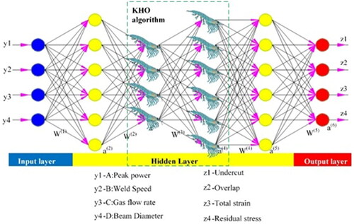
The proposed algorithm was initially trained with 70% and validated with 15% experimental data. The trained DNN-KHO model predicts the remaining 15% of experiment outcomes during the testing process. Then, the optimization of LBW is carried out by giving objective conditions to the DNN-KHO model. Since the optimum LBW process parameters have to be obtained, the objective conditions for all input factors are selected as ‘in range’ conditions. At the same time, strong and light weight weld can be obtained at less stress and strain with minimum undercut and overlap. Hence, the objective condition for all output responses is ‘minimum’.

4. Results and discussion

4.1. Preliminary analysis

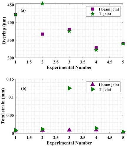
In order to find the best weld joint among ‘I’ and ‘T’, preliminary analyses have been performed. There are five numbers of each ‘I’ and ‘T’ joint specimens made using the ASTM A302 alloy steel plates as per the dimensions shown in Figures 4 and 5. The input parameters such as peak power (W), weld speed (mm/s), gas flow rate (l/min) and beam diameter (mm) are varied, and the changes in output parameters undercut (µm), overlap (µm) and total strain (mm/mm) are noted. Results show that both joints have the same pattern of undercut (µm) and reinforcement (µm) (Figure 10(a)) except for the second experimentation. However, the ‘T’ joint and ‘I’ joint showed different behaviours in terms of total strain (Figure 10(b)). For the same input conditions, the ‘I’ beam total strains are 0.0068, 0.0084, 0.0088, 0.0091 and 0.0032 as well as the ‘T’ total joint strains are 0.0083, 0.0116, 0.1244, 0.014 and 0.0045. These results show that ‘I’ beam offers 18.2%, 27.7%, 92.92%, 36.2% and 29.4% lower strain compared to ‘T’ joints during respective experimentations. Hence, the present investigation chooses the ‘I’ joint for further modelling and optimization.

Figure 10. Preliminary analysis results: (a) overlap and (b) total strain.

4.2. Experimental results

Table 7 shows the various results obtained during the LBW experimentation on ‘I’ beam specimens. The experimentation has been designed using RSM and BBD. There will be four sets (range) of input parameters, peak power (W), weld speed (mm/s), gas flow rate (l/min) and beam diameter (µm), that are identified, and 29 combinations of experimentation are made with the help of RSM. These experimentations are performed in real-time, and the output parameters are measured using respective instruments and displayed in Table 7. The experimentation is looking for improvement in weld quality (i.e. reduction in undercut (µm), overlap (µm)) and a decrease in residual stresses (MPa) and strain (mm/mm). A lower undercut 276 (µm) is achieved during the first experimentation, while the input parameters are 1350 W laser power, 30 mm/s weld speed, 12 l/min argon gas flow rate and 2 mm of the beam diameter. Here, the laser power and the welding speed are used to be the average rate. In contrast, the gas flow rate and beam diameters are set to be at their higher range. For the same experimentation, the overlap was 425 µm, total strain 0.0062 mm/mm and 353.84 MPa. A lower overlap of 216 µm is observed during the 27th experimentation, where the input parameters are 1350 W peak power, 35 mm/s weld speed, 12 l/min of gas flow rate and 1.5 mm of the beam diameter. Further, the RSM-BBD interface is trained using the achieved experimental data. The RSM outcomes are further optimized to satisfy the ANOVA and FIT statistics.

Table 8 shows the RSM-BBD predicted results where the RSM coded model of input/output parameters is shown in Equations (4)–(7). The RSM predictions must satisfy the ANOVA and FIT statistics conditions in order to prove the achieved data to be correct, authentic and fit to the actual experimental situations. Also, the RSM obtained data should be closer enough to the experimental values to show the RSM accuracy in predicting the experimentation. The minimum total strain of 0.0012 mm/mm is observed during the 5th experimentation. For the same experimentation, the RSM predicted total strain value is 0.0022. Here, the error variation is 0.0022–0.0012 = 0.001. This shows the RSM prediction is somewhat close, but the prediction accuracy can be improved. Maximum residual stress of 623.21 MPa is obtained during the 11 experiments. For the same experiment (i.e. same input parametric conditions as the 11th experimental run), the RSM predicted residual stress was 419.92 MPa. This comparison of values shows that the RSM predictions have many deviations compared to the experimental runs. However, different experimental runs show different opinions on the RSM accuracy.

Table 8. RSM predicted results.

		Factor 1	Factor 2	Factor 3	Factor 4	Response 1	Response 2	Response 3	Response 4
		A: peak power	B: weld Speed	C: gas flow rate	D: beam diameter	Undercut	Overlap	Total strain	Residual stress
Std	Run	W	mm/s	l/min	µm	µm	µm	mm/mm	MPa
8	1	1350	30	12	2	473.15	381.656	0.00694	362.95
12	2	1400	30	10	2	372.458	395.217	0.00724	395.66
14	3	1350	35	8	1.5	225.79	430.983	0.00661	421.03
18	4	1400	30	8	1.5	452	374.87	0.00593	366.89
4	5	1400	35	10	1.5	389.1	384.827	0.00219	113.96
15	6	1350	25	12	1.5	401.625	400.203	0.00334	236.95
17	7	1300	30	8	1.5	361.042	327.123	0.00737	450.33
3	8	1300	35	10	1.5	651.52	287.118	0.00593	451.02
28	9	1350	30	10	1.5	752.39	279.99	0.0064	395.24
20	10	1400	30	12	1.5	370.875	336.276	0.0032	166.7
22	11	1350	35	10	1	768.105	291.589	0.00812	419.92
7	12	1350	30	8	2	490.167	341.146	0.012	702.69
25	13	1350	30	10	1.5	749.69	280.65	0.0064	403.55
19	14	1300	30	12	1.5	574.543	341.023	0.00449	302.25
27	15	1350	30	10	1.5	750.412	279.95	0.00639	399.132
23	16	1350	25	10	2	649.708	322.548	0.00835	462.696
10	17	1400	30	10	1	776.792	302.328	0.00412	230.696
9	18	1300	30	10	1	656.958	324.532	0.00799	473.755
6	19	1350	30	12	1	784.52	278.483	0.00853	491.36
13	20	1350	25	8	1.5	818.125	233.147	0.00963	602.3
1	21	1300	25	10	1.5	561	344.895	0.00313	212.73
2	22	1400	25	10	1.5	692.167	290.638	0.00433	336.2
29	23	1350	30	10	1.5	749.85	280.39	0.0064	399.132
21	24	1350	25	10	1	909.042	297.24	0.00693	480.39
26	25	1350	30	10	1.5	791	278.36	0.0064	395.36
24	26	1350	35	10	2	583.877	364.629	0.0081	523.908
16	27	1350	35	12	1.5	815	240.208	0.00729	431.631
11	28	1300	30	10	2	617.602	330.426	0.00617	379.561
5	29	1350	30	8	1	622.59	341.083	0.00908	493.22

4.3. ANOVA analysis

Analysis of variance has to be performed to find the significant terms in the created RSM model and to fine-tune the model accordingly. The ANOVA helps find the fit statistic of the created model as well. Table 9 shows the ANOVA analysis results of output parameters undercut and overlap. For both of these responses, the respective p values are significant, i.e. p values < .0500. This indicates that no insignificant terms exist and no more fine-tuning is required. However, the lack of fit and the FIT statistics must also be considered to confirm the model was good enough and accurate.

Table 9. ANOVA analysis undercut/overlap.

Response 1: undercut					Response 2: overlap
Source	Mean square	F-value	p Value		Mean square	F-value	p Value
Model	61277.68	488.01	<.0001	Significant	4774.89	5733.94	<.0001	Significant
A – peak power	11363.55	90.5	<.0001		1387.59	1666.29	<.0001
B – weld Speed	29827.75	237.55	<.0001		1020.89	1225.94	<.0001
C – gas flow rate	16874.93	134.39	<.0001		414.22	497.42	<.0001
D – beam diameter	1.48E + 05	1175.8	<.0001		7518.36	9028.44	<.0001
AB	38727.68	308.43	<.0001		5773.42	6933.02	<.0001
AC	21701.12	172.83	<.0001		688.91	827.27	<.0001
AD	33302.24	265.22	<.0001		1892.03	2272.05	<.0001
BC	2.53E + 05	2013.8	<.0001		32010.8	38440.2	<.0001
BD	1410.23	11.23	.0048		569.59	683.99	<.0001
CD	8005.51	63.76	<.0001		2657.92	3191.77	<.0001
A^2	1.54E + 05	1223.54	<.0001		7157.11	8594.64	<.0001
B^2	5945.35	47.35	<.0001		1328.52	1595.35	<.0001
C^2	1.76E + 05	1401.78	<.0001		6470.3	7769.87	<.0001
D^2	0.5315	0.0042	.949		3947.03	4739.8	<.0001
Residual	125.57				0.8327
Lack of fit	44.66	0.1362	.995	Not significant	0.8479	1.07	.5191	Not significant
Pure error	327.82				0.7949
Cor total

Lack of fit for undercut and overlap shows 0.995 and 0.5191, respectively. This implies a lack of FIT >0.005 and is not significant. This meant that the lack of fit would not result in a pure error or the derived model fit enough to the actual scenarios.

Table 10 shows the ANOVA analysis of output responses to residual stress (MPa) and total strain (mm/mm). Again, the p values are significant, and the lack of fit shows the model is not significant. This again confirms there is no chance for a pure error, and the derived model fits enough.

Table 10. ANOVA analysis residual stress/total strain.

Response 3: residual stress					Response 4: total strain
Source	Mean square	F-value	p Value		Mean square	F-value	p Value
Model	30743.1	2665.99	<.0001	Significant	9.28E-06	4089.79	<.0001	Significant
A – peak power	36249.4	3143.49	<.0001		5.41E-06	2382.94	<.0001
B – weld speed	76.02	6.59	.0223		5.38E-07	237.08	<.0001
C – gas flow rate	90935.7	7885.79	<.0001		0	10412.9	<.0001
D – beam diameter	4725.25	409.77	<.0001		1.36E-06	598.51	<.0001
AB	53,022	4597.97	<.0001		6.12E-06	2699.05	<.0001
AC	678.86	58.87	<.0001		5.98E-09	2.63	.1269
AD	16790.7	1456.06	<.0001		6.10E-06	2691.07	<.0001
BC	35334.8	3064.17	<.0001		0	5347.32	<.0001
BD	3701.63	321	<.0001		5.17E-07	227.71	<.0001
CD	28540.7	2475	<.0001		5.09E-06	2242.42	<.0001
A^2	79161.9	6864.78	<.0001		0	11,194	<.0001
B^2	507.97	44.05	<.0001		1.60E-06	705.5	<.0001
C^2	7105.09	616.14	<.0001		4.24E-06	1869.23	<.0001
D^2	43253.6	3750.88	<.0001		0	10,921	<.0001
Residual	11.53				2.27E-09
Lack of fit	11.47	0.9802	.5575	not significant	13.17	1.5865	.6345	not significant
Pure error	11.7				2.00E-11
Cor total

4.4. FIT statistics

The FIT statistics show that the regression coefficients (R²) are 0.998, 0.9998, 0.9998 and 0.993 for undercut, overlap, total strain and residual stress, respectively (Table 11). Also, these values look very close to 1. This proves the derived model is reasonable. While the adeq. precision shows 84.7225, 300.7206, 286.1519 and 242.8164 for undercut, overlap, total strain and residual stress, respectively. This implies that the model is desirable and has an adequate signal (the ratio is greater than 4).

Table 11. FIT statistics.

	Undercut	Overlap	Total strain	Residual stress
Std. dev.	11.21	0.9125	0	3.4
Mean	614.18	322.81	0.0065	396.59
CV %	1.82	0.2827	0.7308	0.8562
R^2	0.998	0.9998	0.9998	0.9996
Adjusted R^2	0.9959	0.9997	0.9995	0.9993
Predicted R^2	0.9946	0.9992	0.9986	0.9983
Adeq. precision	84.7225	300.7206	286.1519	242.8164

4.5. Effect of factors and responses

4.5.1. Undercut

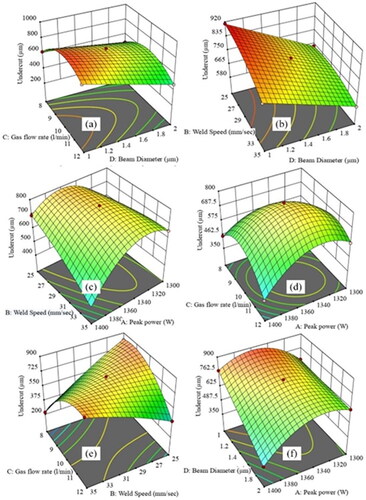
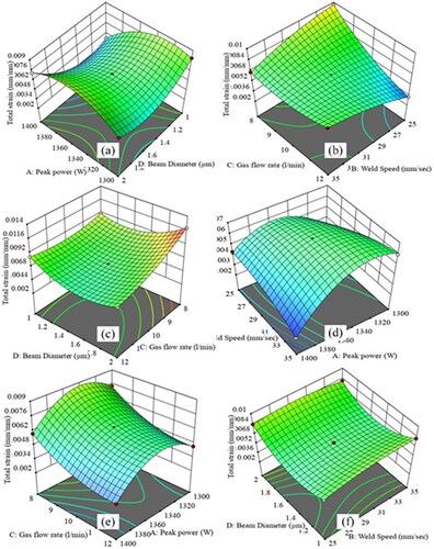
One of the RSM advantages over one factor at a time experimental procedure is its ability to specify the interaction effect between any two factors in the form of three-dimensional (3D) contours. Figure 11 shows the 3D response surface plots of the undercut in which Figure 11(a) represents the undercut response against beam diameter and gas flow rate, Figure 11(b) shows undercut results against beam diameter and weld speed, Figure 11(c) is for undercut versus peak power and weld speed. Similarly, Figure 11(d) shows the rate of change of undercut against peak power and gas flow rate, Figure 11(e) is for undercut responses against weld speed and gas flow rate, Figure 11(f) denotes undercut responses against peak power and beam diameter. From those plots, beam diameter is identified as a highly sensitive parameter on undercut. Whenever the beam diameter is low, the undercut is high, and the maximum undercut is observed when the beam diameter is 1 µm. This is because the higher beam diameter supplies excess energy in the form of heat and force over the weld bead and causes a large penetration, which resulting an undercut in the weld bead region. Also, the large beam diameter occupies more weld bead area than the laser beam, which has a smaller beam diameter. Higher laser power is resulting a lower undercut as the supplied power is effectively used by the laser beam joints and the molten metal in the keyhole area for the successful connection between the materials being joined. The gas flow rate is also closely related to the laser power; however, the welding speed has a different effect. A slow welding speed causes excess energy delivered, resulting in undercut (µm).

Figure 11. RSM surface plot-undercut: (a) beam diameter, gas flow rate, undercut, (b) beam diameter, weld speed, undercut, (c) peak power, weld speed, undercut, (d) peak power, gas flow rate, undercut, (e) weld speed, gas flow rate, undercut and (f) peak power, beam diameter, undercut.

4.5.2. Overlap

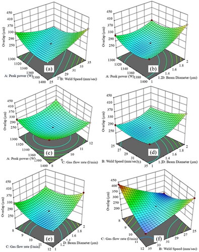
Figure 12 shows the effect of input parameters such as peak power, weld speed, gas flow rate and beam diameter on overlap (µm). Overlap is a defect in the weld bead where the weldment is projected outside the welded region. The overlap parameter should be minimized for improved weld quality and optimal conditions. The RSM experimentation shows interesting results regarding the input parameters and the overlap relation. From Figure 12(a–f), all input parameters look to have the same response pattern on the overlap. However, comparatively beam diameter has the least effect on the overlap. From RSM surface plots, it can be seen an average rate of input parameters tends to sufficient penetration, which leads to the rise of weldment in the required proportion. A higher welding speed causes lower energy deepening in the region being welded, causing the overlap projection. In contrast, a high gas flow rate controls the overlap by the effective penetration and heat utilization in the welded region.

Figure 12. Response surface plot–overlap: (a) weld speed, peak power, overlap, (b) beam diameter, peak power, overlap, (c) gas flow rate, peak power, overlap, (d) weld speed, beam diameter, overlap, (e) gas flow rate, beam diameter, overlap and (f) weld speed, gas flow rate, overlap.

4.5.3. Total strain

Figure 13(a–f) shows the effect of LBW input parameters on the output response total strain mm/mm. The curvilinear relationship between total strain and all input factors was noticed by analysing total strain 3D contour. The maximum strain was observed in Figure 13(c), which is plotted against beam diameter and gas flow rate. It was evident that the gas flow rate and beam diameter are the most influencing parameters on strain development during the study. Whereas, the lowest value and less influencing factors for total strain are noticed in Figure 13(d), which is plotted against weld speed and peak power. The reason for those observed higher strain values may be the strength reduction in weld bead during the lower weld diameter and the rise of other defects such as overlap (reinforcement) and undercut. However, the average range of gas flow rate and beam diameter offers optimal total strain. Peak power has a lower effect on total strain at its maximum state. This shows power contributes more to making the most strengthened LBW joints.

Figure 13. Response surface plot—total strain: (a) beam diameter, peak power, total strain, (b) weld speed, gas flow rate, total strain, (c) gas flow rate, beam diameter, total strain, (d) peak power, weld speed, total strain, (e) peak power, gas flow rate, total strain and (f) weld speed, beam diameter, total strain.

4.5.4. Residual stress

Similarly, the difference in residual stress formation obtained from RSM method is differentiated by colour gradient method. The yellowish red colour in Figure 14 indicates maximum stress formation, whereas the blue colour indicates lower values of stress. In terms of residual stress (MPa), the peak power and the gas flow rate are reducing factors, as per Figure 14. While increasing the gas flow rate with reduced peak power significantly reduced the residual stress formation (Figure 14(a,b)), this reduced stress formation occurs due to lower temperature concentration in the weld zone at low peak power and a simultaneous reduction in generated heat due to high gas flow rate. Because the heat generated during the welding process is an important factor in the rate of change of residual stresses around the weld bead region.

Figure 14. Response surface plot—residual stress. (a) Peak power, weld speed, residual stress, (b) peak power, gas flow rate, residual stress, (c) peak power, beam diameters, residual stress, (d) weld speed, beam diameters, residual stress, (e) weld speed, gas flow rate, residual stress and (f) gas flow rate, beam diameter, residual stress.

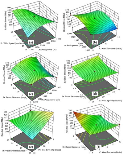
On the other hand, the increased gas flow rate and peak power together increase the weld bead temperature, width and penetration. This leads to higher bond between the molecules in joining region thereby achieving high-strength joint. Meanwhile, the high beam diameter results in high temperature distortion around the heat affected zone thus increasing residual stress (MPa) as noticed in Figure 14(f). According to Figure 14(e), lower weld speed along with less gas flow rate considerably increased the residual stress formation due to increased heat distortion on welded specimen. Whereas, Figure 14(c,d) shows midrange of residual stress formation, indicating that the residual stress was comparatively less sensitive to the combined effect of beam diameter-peak power and beam diameter-weld speed. This scenario perfectly matches the experimental observation, where the residual stress values are not much affected by increasing peak power and weld speed along with beam diameter.

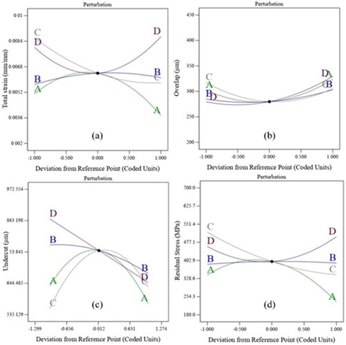
4.6. Perturbation analysis

Perturbation analysis is one of the outcomes achieved from the RSM. After the response surface plots, the perturbation plots help determine the effect of individual input parameters on the output parameters. Here, Figure 15(a) shows the effect of input parameters on total strain (mm/mm), Figure 15(b) shows the effect of input parameters on overlap (µm), Figure 15(c) shows the effect of input parameters on undercut (µm) and Figure 15(d) shows the effect of input parameters on residual stress (MPa). From these plots, the optimal state of output parameters lies somewhere in the middle range of individual input parameters. Also, Figure 15 allows to comprehensively analyse all output responses each other against input factors. As a result, similar trend against input factors was noticed for residual stress and total strain measurements. Whereas, overlap is less sensitive for all input factors and undercut is more sensitive for the factors peak power and weld speed, respectively. From RSM, response surface plots and perturbation plots, the optimal LBW parameters were undercut 791 µm, peak power 1350 W, weld speed 30 mm/s, gas flow rate 10 l/min and beam diameter 1.5 mm. These values are obtained during the 25th experimental run, where the corresponding output parameters are undercut 791 µm, overlap 278.36 µm, total strain 0.0064 mm/mm and residual stress 395.36 MPa.

Figure 15. Perturbation plots. (a) Total strain (mm/mm), (b) overlap (µm), (c) undercut (µm) and (d) residual stress (MPa).

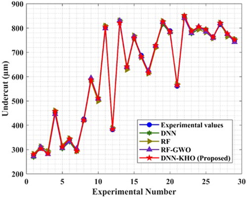
4.7. Deep neural network based Krill Herd optimizer prediction results

Different ‘I’ section laser weld parameters are predicted using the DNN-KHO algorithm and compared with other existing algorithms such as non-hybrid DNN, random forest method and hybrid random forest-grey wolf optimizer (RF-GWO). From Figure 16, during the first experimental run, the lowest undercut of 273.27 µm was predicted by the proposed DNN-KHO. During this experimentation, the input parameters are 1350, 30, 12 and 2, respectively, peak power (W), weld speed (mm/s), gas flow rate (l/min) and beam diameter (µm). From the same experimentation, the undercut predicted by other parameters are 286.189 µm, 284.57 µm and 255.212, respectively, predicted by RF-GWO, RF and DNN. While the actual (experimental) undercut value for the respective experimental run will be 276 µm. Here, the proposed DNN provided the closest result by predicting an undercut by 286.189 µm. It shows the proposed DNN-KHO algorithm provided the closest result to other algorithms used in the comparison.

Figure 16. DNN-KHO predicted undercut.

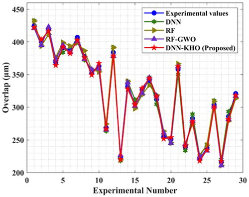
Figure 17 compares different algorithms for predicting the LBW overlap parameter versus proposed DNN-KHO predictions. Here, the lowest overlap of 211.27 µm is predicted by the proposed DNN-KHO during the 27 experimental runs. At the same time, the respective input parameters are 1350 W, 35 mm/s, 12 l/min and 1.5 mm, respectively, peak power, weld speed, gas flow rate and beam diameter. The other predicted values for the same input parameters are 221.73 µm, 224.74 µm and 229.679 µm, respectively, by RF-GWO, RF and DNN. Here again, the proposed method DNN-KHO performed better by predicting the closest result to the experimental value of 216 µm. The proposed method predicted the higher overlap (reinforcement) value during the first experimental run to be 420.66 µm.

Figure 17. DNN-KHO predicted overlap.

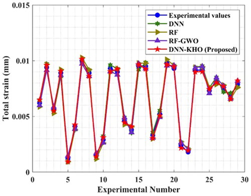
The respective total strain (mm/mm) predicted by the DNN-KHO is 0.006, 0.010, 0.006, 0.009, 0.001, 0.004, 0.010, 0.009, 0.001, 0.003, 0.009, 0.009, 0.005, 0.004, 0.009, 0.010, 0.004, 0.005, 0.010, 0.010, 0.002, 0.002, 0.009, 0.009, 0.007, 0.008, 0.008, 0.007 and 0.008 (numbers were formatted to an accuracy of 0.000) during the experimentations starting from 1 to 29. Here, the lowest strain of 0.001008 mm/mm is recorded during the 5th experimentation, where the peak power is 1400 W, weld speed is 35 mm/s, gas flow rate is 10 l/min and beam diameter is 1.5 mm. Meanwhile, for the same experimentation, respective RF-GWO, RF and DNN predicted strain values are 0.0015, 0.00093 and 0.0015. The values predicted by different algorithms are close to each other. However, the DNN-KHO prediction is close to the experimental value (0.0012 mm/mm) compared to the perdition behaviour of other existing algorithms. While a high strain of 0.009819 is recorded during the 7th experimentation, the input parameters are peak power of 1300 W, weld speed of 30 mm/s, gas flow rate of 8 l/min and beam diameters of 1.5 mm. Figure 18 shows the prediction (total strain) results of various algorithms. Figure 18 shows the prediction behaviours of different algorithms on total strain mm/mm.

Figure 18. DNN-KHO predicted total strain.

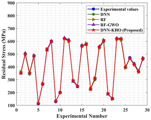
Figure 19 shows the comparison of predicted results on residual stress (MPa). Here, the DNN-KHO predicted results are 355.98, 504.32, 343.30, 487.32, 110.84, 262.53, 535.63, 604.71, 123.79, 198.33, 628.92, 610.38, 293.67, 248.73, 561.76, 584.30, 232.24, 303.90, 556.00, 606.04, 192.40, 153.84, 617.50, 621.82, 399.75, 470.35, 416.10, 369.87 and 466.63 Mpa, respectively, during the experimental runs from 1 to 29. Here, the lowest residual stress of 110.84 MPa is observed during the 5th experimentation, where the input parameters will be peak power of 1400 W, weld speed of 35 mm/s, gas flow rate of 10 l/min and beam diameter of 1.5 µm. For the same input parameters, the respective predicted results performed by the existing algorithms RF-GWO, RF and DNN are 119.377 MPa, 103.558 MPa and 126.890 MPa. Here, the proposed algorithm DNN-KHO provided comparatively close results (110.84 MPa) to the experimental results (112.23 MPa). Next to that, the RF-GWO provided competitive results (119.377 MPa). These predictions show that the proposed algorithm DNN-KHO performed better than other algorithms used in the present investigation.

Figure 19. DNN-KHO predicted residual stress.

4.8. Root mean square error (RMSE) analysis

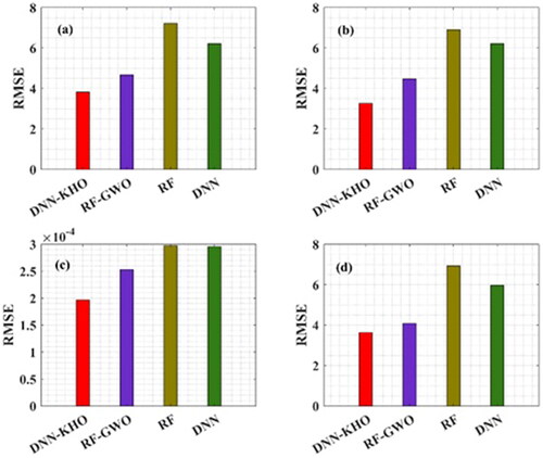
The root mean square analysis is a great tool to see how the results of different comparison algorithms deviate from the experimental values. Here, the respective RMSE values of the DNN-KHO algorithm are 2.98, 3.66, 0.00020 and 3.53 for undercut, overlap, total strain and residual stress. In contrast, the respective RSME analysis results of RF-GWO predictions are 4.61, 4.17, 0.00025 and 4.41. This shows that the RF-GWO predictions are the closest to DNN-KHO predictions compared to non-hybrid-RF and DNN methods. In overall, from the plots below in Figure 20(a–d), the proposed algorithm performed the best among all other algorithms providing the closest results as experimental results and least deviations. The hybrid RF-GWO algorithm was found to be showing competitive results.

Figure 20. Root mean square (RMSE) analysis for (a) undercut, (b) overlap, (c) total strain and (d) residual stress.

4.9. Optimal parameters observed from DNN-KHO

Finally, the optimization task has been performed by the hybrid DNN-KHO algorithm. The weld outcomes such as overlap (µm), undercut (µm), total strain (mm/mm) and residual stress (MPa) should be limited or minimum to achieve high quality weld bead behaviours. Therefore, the objective conditions of all output responses for generating optimal LBW parameters are given as minimum. Table 12 shows the optimized LBW process parameters and their respective outcomes. The proposed algorithm optimized the results within 15–20 iterations or loops with an above 0.99 regression coefficient for all output responses.

Table 12. LBW optimized process parameters.

Algorithm	Peak power (W)	Weld speed (mm/s)	Gas flow rate (l/min)	Beam diameter (µm)	Undercut (µm)	Overlap (µm)	Total strain (mm/mm)	Residual stress (MPa)
DNN-KHO	1362	28.2	10.6	1.3	280.21	218.16	0.00199	168.15

5. Conclusions

The development of residual stress, strain and defects during the LBW process of vehicle chassis parts is a problem. The chassis members should be compact in design, weightless, fit into the existing designs, and bear different load conditions. Hence, LBW is performed on ASTM A302 alloy steel material, and the effect of different process parameters and input variable on output responses are studied. In order to do so, various techniques such as advanced ND based inspecting instruments, RSM, neural network based prediction and optimization processes are implemented. Besides, the experimentation has been predicted using hybrid DNN-KHO, and the results are compared using different algorithms.

• During the preliminary analysis, the ‘I’ section and the ‘T’ section are evaluated for load carrying capacity and the strain rate caused by the applied load. Preliminary analysis shows that the ‘I’ beam offered 18.2%, 27.7%, 92.92%, 36.2% and 29.4% lower strain during respective experimentations compared to the ‘T’ joint configuration. This confirms that the ‘I’ sections have high load carrying capacity while offering less strain. Hence, further experimentation has been conducted on the ‘I’ beam configuration, which has four Butt weld joints.

• The experimentation has been designed using RSM, BBD. In addition, ANOVA analysis and FIT statistics are performed to validate the designs’ authenticity. ANOVA analysis was not significant from lack of fit by 0.995, 0.5191, 0.5575 and 0.6345, respectively, for undercut, overlap, residual stress and total strain.

• A higher beam diameter delivers excess energy over the weld bead causing a high penetration depth and building weld geometry defects such as undercut. In contrast, a higher laser power limits the penetration and promotes the formation of a high quality weld bead.

• The beam diameter has the least effect on the reinforcement or overlap. But the welding speed was found to reduce penetration depth and take responsibility for forming overlap. While a moderate weld speed with a bit higher gas flow rate leads to better weld bead form. And a higher beam diameter creates more residual stresses in the region.

• The proposed DNN-KHO algorithm outperformed the prediction behaviour of other existing algorithms, such as RF-GWO, RF and DNN, by 21.53%, 45.428% and 41.31%, respectively, meaning that the proposed algorithm provided the closest results to the experimental data.

• Finally, LBW process parameters have been optimized using the DNN-KHO algorithm. The optimal parameters are achieved between 15 and 20 iterations, such as peak power 1362 (W), weld speed 28.2 (mm/s), gas flow rate 10.6 (l/min), beam diameter 1.3 µm, undercut 280.21 µm, overlap 218.16 µm, total strain 0.00199 mm/mm, residual stress 168.15 MPa, respectively.

Thus, the strength of weld joints made on the ‘I’ section chassis member was examined regarding weld bead geometry and residual stress and strain developed by LBW. The welding parameters considered for the study are limited due to the length and complexity of the study. This limitation can be solved in future works by considering more input factors like the type of shielding gas, focal point, laser angle, etc. Moreover, this study can motivate readers to extend the study by analysing the morphology of weld bead using SEM or XRD methods that are not focused on in this study.

Disclosure statement

The authors declare that they have no conflict of interest.

Data availability statement

Data sharing do not apply to this article.

Additional information

Funding

No funding is provided for the preparation of the manuscript.

References

- Leggatt RH. Residual stresses in welded structures. Int J Press Vessel Pip. 2008;85(3):144–151. doi: 10.1016/j.ijpvp.2007.10.004
- Rossini NS, Dassisti M, Benyounis K, et al. Methods of measuring residual stresses in components. Mater Des. 2012;35:572–588. doi: 10.1016/j.matdes.2011.08.022
- Tankova T, da Silva LS, Balakrishnam M, et al. Residual stresses in welded I section steel members. Eng Struct. 2019;197:109398. doi: 10.1016/j.engstruct.2019.109398
- Derakhshan ED, Yazdian N, Craft B, et al. Numerical simulation and experimental validation of residual stress and welding distortion induced by laser-based welding processes of thin structural steel plates in butt joint configuration. Opt Laser Technol. 2018;104:170–182. doi: 10.1016/j.optlastec.2018.02.026
- Yu J, Kim D. Effects of welding current and torch position parameters on minimizing the weld porosity of zinc-coated steel. Int J Adv Manuf Technol. 2018;95(1–4):551–567. doi: 10.1007/s00170-017-1180-6
- Ozerov M, Povolyaeva E, Stepanov N, et al. Laser beam welding of a Ti–15Mo/TiB metal–matrix composite. Metals. 2021;11(3):506. doi: 10.3390/met11030506
- Svensson LE, Karlsson L, Söder R. Welding enabling light weight design of heavy vehicle chassis. Sci Technol Weld Join. 2015;20(6):473–482. doi: 10.1179/1362171814Y.0000000269
- Moaaz AO, Ghazaly NM. A review of the fatigue analysis of heavy duty truck frames. Am J Eng Res. 2014;3(10):1–6.
- Chen K, Chen H, Liu L, et al. Prediction of weld bead geometry of MAG welding based on XGBoost algorithm. Int J Adv Manuf Technol. 2019;101(9–12):2283–2295. doi: 10.1007/s00170-018-3083-6
- Withers PJ. Residual stress and its role in failure. Rep Prog Phys. 2007;70(12):2211–2264. doi: 10.1088/0034-4885/70/12/R04
- Dong P. Residual stresses and distortions in welded structures: a perspective for engineering applications. Sci Technol Weld Join. 2005;10(4):389–398. doi: 10.1179/174329305X29465
- Junaid M, Khan FN, Rahman K, et al. Effect of laser welding process on the microstructure, mechanical properties and residual stresses in Ti–5Al–2.5 Sn alloy. Opt Laser Technol. 2017;97:405–419. doi: 10.1016/j.optlastec.2017.07.010
- Franco A, Romoli L, Musacchio A. Modelling for predicting seam geometry in laser beam welding of stainless steel. Int J Therm Sci. 2014;79:194–205. doi: 10.1016/j.ijthermalsci.2014.01.003
- Wits WW, Becker JJ. Laser beam welding of titanium additive manufactured parts. Proc CIRP. 2015;28:70–75. doi: 10.1016/j.procir.2015.04.013
- Jelokhani-Niaraki MR, Arab NBM, Naffakh-Moosavy H, et al. The systematic parameter optimization in the Nd:YAG laser beam welding of inconel 625. Int J Adv Manuf Technol. 2016;84(9–12):2537–2546. doi: 10.1007/s00170-015-7833-4
- Satyanarayana G, Narayana KL, Rao BN. Identification of optimum laser beam welding process parameters for E110 zirconium alloy butt joint based on Taguchi-CFD simulations. Lasers Manuf Mater Process. 2018;5(2):182–199. doi: 10.1007/s40516-018-0061-7
- Myers RH, Dc M, Cm A-C. Response surface methodology: process and product optimization using designed experiments. John Wiley & Sons; 2016.
- Chelladurai SJS, Murugan K, Ray AP, et al. Optimization of process parameters using response surface methodology: a review. Mater Today Proc. 2021;37:1301–1304.
- Yolmeh M, Jafari SM. Applications of response surface methodology in the food industry processes. Food Bioprocess Technol. 2017;10(3):413–433. doi: 10.1007/s11947-016-1855-2
- Torabi A, Kolahan F. Optimizing pulsed Nd:YAG laser beam welding process parameters to attain maximum ultimate tensile strength for thin AISI316L sheet using response surface methodology and simulated annealing algorithm. Opt Laser Technol. 2018;103:300–310. doi: 10.1016/j.optlastec.2017.12.042
- Shanmugarajan B, Shrivastava R, Sathiya P, et al. Optimization of laser welding parameters for welding of P92 material using Taguchi based grey relational analysis. Defence Technol. 2016;12(4):343–350. doi: 10.1016/j.dt.2016.04.001
- Tutar M, Aydin H, Yuce C, et al. The optimization of process parameters for friction stir spot-welded AA3003-H12 aluminium alloy using a Taguchi orthogonal array. Mater Des. 2014;63:789–797. doi: 10.1016/j.matdes.2014.07.003
- Schmidt PA, Pauleser T, Zaeh MF. Optimization of weld seam configurations using a genetic algorithm. Proc CIRP. 2014;25:393–399. doi: 10.1016/j.procir.2014.10.054
- Sibalija TV. Particle swarm optimization in designing parameters of manufacturing processes: a review (2008–2018). Appl Soft Comput. 2019;84:105743. doi: 10.1016/j.asoc.2019.105743
- Dabhade S, Dabhade O, Kolekar N, et al. Design and analysis of TATA 2518 TC chassis frame. Int J Res Eng Sci Manage. 2019;2(1):478–480.
- Taraphdar PK, Thakare JG, Pandey C, et al. Novel residual stress measurement technique to evaluate through thickness residual stress fields. Mater Lett. 2020;277:128347. doi: 10.1016/j.matlet.2020.128347
- Palanichamy P, Vasudevan M, Jayakumar T. Measurement of residual stresses in austenitic stainless steel weld joints using ultrasonic technique. Sci Technol Weld Join. 2009;14(2):166–171. doi: 10.1179/136217108X394753
- Hill WJ, Hunter WG. A review of response surface methodology: a literature survey. Technometrics. 1966;8(4):571–590. doi: 10.2307/1266632
- Khuri AI, Mukhopadhyay S. Response surface methodology. WIREs Comp Stat. 2010;2(2):128–149. doi: 10.1002/wics.73
- Myers RH, Khuri AI, Carter WH. Response surface methodology: 1966–1988. Technometrics. 1989;31(2):137–157.
- Krizhevsky A, Sutskever I, Hinton GE. ImageNet classification with deep convolutional neural networks. Proceedings of the Advances in Neural Information Processing Systems (NIPS); 2012. p. 1097–1105.
- Ciresan D, Giusti A, Gambardella LM, et al. Deep neural networks segment neuronal membranes in electron microscopy images. Proceedings of the Advances in Neural Information Processing Systems (NIPS); 2012. p. 2852–2860.
- Szegedy C, Liu W, Jia Y, et al. Going deeper with convolutions [Online]; 2014. Available from: http://arxiv.org/abs/1409.4842
- Ciregan D, Meier U, Schmidhuber J. Multi-column deep neural networks for image classification. Proceedings of the IEEE Computer Vision and Pattern Recognition; 2012. p. 3642–3649.
- Collobert R, Weston J, Bottou L, et al. Natural language processing (almost) from scratch. J Mach Learn Res. 2011;12:2493–2537.
- Socher R, Perelygin A, Wu J, et al. Recursive deep models for semantic compositionality over a sentiment treebank. Proceedings of the Empirical Methods in Natural Language Processing (EMNLP); 2013. p. 1631–1642.
- Liu W, Wang Z, Liu X, et al. A survey of deep neural network architectures and their applications. Neurocomputing. 2017;234:11–26. doi: 10.1016/j.neucom.2016.12.038
- Serre T, Kreiman G, Kouh M, et al. A quantitative theory of immediate visual recognition. Prog Brain Res. 2007;165:33–56.
- Bengio Y, Lamblin P, Popovici D, et al. Greedy layer-wise training of deep networks. Adv Neural Inf Process Syst. 2007;19:153.
- Wang GG, Guo L, Gandomi AH, et al. Chaotic Krill Herd algorithm. Inf Sci. 2014;274:17–34. doi: 10.1016/j.ins.2014.02.123
- Wang GG, Gandomi AH, Alavi AH. Stud Krill Herd algorithm. Neurocomputing. 2014;128:363–370. doi: 10.1016/j.neucom.2013.08.031
- Bolaji ALA, Al-Betar MA, Awadallah MA, et al. A comprehensive review: Krill Herd algorithm (KH) and its applications. Appl Soft Comput. 2016;49:437–446. doi: 10.1016/j.asoc.2016.08.041
- Guo L, Wang GG, Gandomi AH, et al. A new improved Krill Herd algorithm for global numerical optimization. Neurocomputing. 2014;138:392–402. doi: 10.1016/j.neucom.2014.01.023
- Wang GG, Gandomi AH, Alavi AH, et al. A comprehensive review of Krill Herd algorithm: variants, hybrids and applications. Artif Intell Rev. 2019;51(1):119–148. doi: 10.1007/s10462-017-9559-1
- Abualigah LM, Khader AT, Hanandeh ES. Hybrid clustering analysis using improved Krill Herd algorithm. Appl Intell. 2018;48(11):4047–4071. doi: 10.1007/s10489-018-1190-6
- Gandomi AH, Alavi AH. Krill Herd: a new bio-inspired optimization algorithm. Commun Nonlinear Sci Numer Simul. 2012;17(12):4831–4845. doi: 10.1016/j.cnsns.2012.05.010