Reinforcement learning based optimal decision making towards product lifecycle sustainability

ABSTRACT

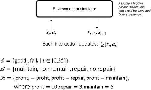
Artificial intelligence (AI) has been widely used in robotics, automation, finance, healthcare, etc. However, using AI for decision-making in sustainable product lifecycle operations is still challenging. One major challenge relates to the scarcity and uncertainties of data across the product lifecycle. This paper aims to develop a method that can adopt the most suitable AI techniques to support decision-making for sustainable operations based on the available lifecycle data. It identifies the key lifecycle stages in which AI, especially reinforcement learning (RL), can support decision-making. Then, a generalised procedure of using RL for decision support is proposed based on available lifecycle data, such as operation and maintenance data. The method has been validated in a case study of an international vehicle manufacturer, combined with modelling and simulation. The case study demonstrates the effectiveness of the method and identifies that RL is the current most appropriate method for maintenance scheduling based on limited available lifecycle data. This paper contributes to knowledge by demonstrating an empirically grounded industrial case using RL to optimise decision-making for improved product lifecycle sustainability by effectively prolonging the product lifetime and reducing environmental impact.

KEYWORDS:

• Artificial intelligence
• reinforcement learning
• decision-making
• sustainability
• lifecycle

1. Introduction

Manufacturing is facing a new, exciting era due to the emergence of new technologies, such as the Internet of Things (IoT) (Cai et al. 2014; Zhang et al. 2018), big data analytics (BDA) (Ren et al. 2019; Zhang et al. 2017a), cloud computing (Talhi et al. 2019), artificial intelligence (AI) (Liu et al. 2020b) and digital twin (Tao et al. 2018). Many researchers and practitioners consider these technologies and powerful tools to make manufacturing more efficient, profitable and sustainable (Guo et al. 2021b; Wang et al. 2020). There is an increasing interest from academia and industries using these technologies for a more sustainable operation and supply chain in manufacturing. This can be achieved by better planning, designing, and maintaining the production system, product, and service. For instance, a large volume of data is generated in different product lifecycle phases with various degrees of complexity (Lou et al. 2018) and has been used to improve the product/service design, enhance the production performance of the shop floor and carry out predictive maintenance (Zhang et al. 2017b). This could vastly improve sustainable operations, especially in the economic and environmental dimensions, through better decision-making and planning.

Most of the existing studies are based on data-driven modelling and multi-objective optimisation for sustainable operations. For example, Hatim et al. (2020) presented a multi-criteria decision-making method for the globalised assessment of sustainability and productivity in the integrated process and operation plans. In addition, Meng et al. (2020) reviewed the state-of-art of smart recovery decision-making for end-of-life products and highlighted the contribution of ubiquitous information and computational intelligence. These emerging smart technologies not only reduce the information uncertainties but also provide powerful operational methodologies. Nevertheless, few studies utilise the power of advanced AI techniques to extract valuable information and knowledge from limited available data and further process the data to support decision-making towards sustainability (Govindan, Jafarian, and Nourbakhsh 2019; Nishant, Kennedy, and Corbett 2020; Jarrahi 2018).

The purpose of this paper is to examine how AI can improve the product lifecycle sustainability, such that failures are minimised, lifetime increased, and ultimately that financial and environmental costs are reduced. AI techniques hold great promise in automating and improving several aspects of this process, e.g. predicting breakdowns and planning maintenance schedules in advance. To utilise AI to support decision making throughout the lifecycle, the isolated lifecycle data that influence the system design, product, and service need to be integrated and analysed to generate important insights. Besides, AI offers further opportunities to gain insight into data to perceive and predict future trends for better planning accurately, accelerate market development, and design sustainable products and services. It can also help decision-makers identify the most important and valuable features based on concrete customer inputs and designs that minimise production costs and harness consumer insights to reduce development costs. Furthermore, it can also help improve the product and service design for purposes, such as design for reliability, maintenance, remanufacturing, etc. The study was done through a 3-year Swedish state-funded project with three participating companies, which produce vehicles, aeroplanes, and integrated systems solutions.

This paper investigates the application of AI techniques for decision-making towards sustainable operations in product lifecycle phases. Firstly, the key stages in which AI can support decision-making were identified. Then, the authors focused on typical cases and proposed a generalised method and procedure with AI for decision support using lifecycle data (such as data obtained from operations and maintenance) that can be useful to improve sustainability. Specifically, reinforcement learning (RL) was applied to optimise decision-making based on limited available lifecycle data and validated through a real industrial case study. An illustrative case study, combining with modelling and simulation, is conducted to demonstrate the feasibility and performance of the proposed method using AI to improve decision-making in the middle of life stage scenario. A similar method can be expanded to other lifecycle stages and cover the whole lifecycle if necessary.

The rest of the paper is organised as follows. Section 2 reviews the state-of-the-art literature. Section 3 develops the relevant theoretical reasoning. Section 4 presents an AI system for decision-making focusing on maintenance. Section 5 presents an illustrative case study based on RL for operations and maintenance. Section 6 concludes the paper.

2. Literature review

AI has existed for decades and has been widely used in different areas such as robotics, automation, finance and healthcare. The new technological revolution and the new industrial revolution fusing new AI technologies are characterised by ubiquitous networks, data-drivenness, shared services, cross-border integration, automatic intelligence, and mass innovation (Li et al. 2017). Duan, Edwards, and Dwivedi (2019) reviewed the history of AI and its decision-making issues regarding the interaction and integration of AI to support or replace human decision-makers. The relationship between AI and decision-making has been systematically discussed by Pomerol (1997), which includes diagnosis (expert systems, case-based reasoning, fuzzy set, and rough set theories) and look-ahead reasoning with uncertainty and preferences. Jarrahi (2018) highlighted the complementarity of humans and AI in organisational decision-making processes with uncertainty, complexity, and equivocality. In large-scale decision-making (LSDM) scenarios, multiple and highly diverse stakeholders/decision-makers and the timeliness of information dissemination further increase the complexity of decision-making problems. The definition and characterisation of LSDM events have been proposed by Ding et al. (2020).

AI has also been used to facilitate capturing, structuring and analysing big data for key insights (O’Leary 2013), especially in the area of product lifecycle management (PLM). For example, smart embedded systems can gather data through a product lifecycle for decision-making, including adaptive production management for the beginning of life (BOL), predictive maintenance for the middle of life (MOL) and planning and management for the end of life (EOL) (Kiritsis, Bufardi, and Xirouchakis 2003). The various data involved in the three main phases of PLM, i.e. BOL, MOL, and EOL, are analysed by big data techniques to enhance the intelligence and efficiency of design, production, and service processes (Li et al. 2015). Methodologies and software architecture have been presented to integrate enterprise-wide applications with new functionality to enable knowledge-based contemporary design at the conceptual design phase (Gao et al. 2003). To meet the openness, interoperability, and decentralisation requirements, an industrial blockchain-based PLM framework has been proposed to facilitate data exchange and service sharing in the product lifecycle (Liu et al. 2020a).

As effective decision-making is vital for the management of product portfolios and related data across all phases of the product lifecycle, MacCarthy and Pasley (2021) proposed the concept of group decision support for the reuse of decision information to achieve effective PLM. In terms of performance and value indicators based on knowledge management integration, Bosch-Mauchand et al. (2013) presented a PLM approach to support knowledge capture for reuse purposes and to assess managerial and technical decisions. In engineering applications, Lee et al. (2008) discussed the evolution of PLM and reviewed the characteristics and benefits of PLM and its practices and potential applications in aviation maintenance, repair and overhaul (MRO). From a PLM perspective, the benefits of digital twin (DT) have also been reviewed to reflect the physical status of systems or products in a virtual space (Lim, Zheng, and Chen 2020). Additionally, Matsokis and Kiritsis (2010) developed an ontology model of product data and knowledge management semantic object model for PLM to implement ontology advantages and features. Under incomplete information and constraints, Andriotis and Papakonstantinou (2020) proposed a joint framework of constrained partially observable Markov decision processes and multi-agent deep reinforcement learning to solve inspection and maintenance planning problems.

Despite the significant progress, few existing methods leverage AI to support the decision-making for sustainable PLM due to the lack of data and various uncertainties. Using AI for decision-making in operations is still challenging and less popular due to three reasons: 1) the lack of sufficient ‘good’ data to be useful for AI algorithms to process and obtain meaningful results; 2) cleaning of ‘bad’ data usually takes more efforts than the AI algorithms themselves, and so far there is no simple way to solve it automatically but rather manually instead, which greatly demotivate and reduce the value of using AI; 3) using AI to process the qualitative information required by decision-making is challenging. Consequently, applying AI to optimise decision-making throughout lifecycle phases to achieve better sustainability is still in its infancy. Overall, an AI-based optimal decision-making method considering data scarcity and uncertainties towards sustainable PLM needs to be further developed, which is a niche that this paper aims for and positions its contribution.

A comparison of the most relevant literature on the decision-making for sustainable PLM is given in Table 1. From the table, advanced techniques such as big data analytics, digital twin, reinforcement learning, and blockchain have been used to support the decision-making for sustainable PLM. The works searched were published in the recent five years (2017–2021) and received at least one citation from the Web of Science.

Table 1. Summary of the literature on the decision-making for product lifecycle management.

Reference	Area	Decision process	Key technique	Data source
Zhang et al. (2017b)	Manufacturing industry	Maintenance service stage	Big data analytics	Onsite observations, interviews and reports
Ferreira et al. (2017)	Automotive industry	Planning, machining and evaluation stages	Knowledge-based collaborative processes	Original equipment manufacturers and suppliers
Rondini et al. (2017)	Automotive industry	Maintenance service stage	Discrete event simulation with agent-based modelling	Truck maintenance company
Badurdeen, Aydin, and Brown (2018)	Manufacturing industry	Product design stage	Non-dominated sorting genetic algorithm II	Toner cartridge company
Kaewunruen and Lian (2019)	Infrastructure industry	Planning and design, manufacturing, pre-assembly, logistic, reconstruction and installation, operation and maintenance, demolition and recycle/renewal stages	Digital twin (building Information modelling)	Raw data from the field
Li, Zhong, and Lin (2019)	Aero-engine maintenance	Maintenance service stage	Reinforcement learning	Hypothetical data
Yao et al. (2020)	Infrastructure industry	Maintenance service stage	Deep reinforcement learning	Expressway data
Yousefi, Tsianikas, and Coit (2020)	Dynamic maintenance policy	Maintenance service stage	Reinforcement learning	Hypothetical data
Liu et al. (2020a)	Manufacturing industry	Co-creation, tracking and tracing, maintenance and recycling service stages	Industrial blockchain	Smart gateway by IoT sensors and RFID
Andriotis and Papakonstantinou (2020)	Inspection and maintenance planning	Maintenance service stage	Deep reinforcement learning	Hypothetical data
This paper	Manufacturing industry	Middle of life stage (operation and maintenance) with environmental impacts	Reinforcement learning	Empirical data of the case company with limited availability

It can be seen that this paper clearly differs from other works as follows. 1) The data of this paper came from real industry, and the proposed method was empirically applied with action research. 2) The AI-based decision process in this paper covered a wider lifecycle stage. 3) This paper also contributed to sustainability goals, particularly prolonging the product lifetime and reducing environmental impact.

3. Theoretical development

3.1 AI for decision making towards sustainability

The general goals of using AI to optimise sustainability lie in the economic, environmental and social dimensions. The economic goal is to maximise the profit of the provider while minimising the cost to the consumer. The environmental goal is to provide resource-efficient and effective solutions to minimise environmental impact. The social goal is to minimise human efforts to reach near-optimal results and improve wellbeing.

AI has the potential to help improve decision-making towards sustainability in service-oriented business models, i.e. product-service systems (PSS), which are widely used in specific industries, e.g. vehicles, aircraft engines, production machines. The rental business model, for example, currently still suffers from high cost and low sustainability compared to the traditional selling model, but the societal and political needs accelerate the transition from ownership to access (Geissinger et al. 2019; Rifkin 2000), especially in the automobile sector (Ma et al. 2018; Wingfield 2017). The business model is not optimised for sustainability because the product (i.e. the car) used is not designed and optimised throughout the lifecycle for such a business model but rather for the traditional ownership model. There is a need to redesign and optimise the product to adapt to the new business model. AI is widely considered to have great potential in many kinds of optimisations. However, the lack of knowledge makes it extremely challenging. AI experts do not believe so because AI relies heavily on existing data and domain knowledge, but they do not exist in this case. However, the authors of this paper propose a new approach to making this possible.

3.2 AI for PSS decision making

AI can be used to optimise decisions in the design of the optimal offerings, particularly in the PSS model, to maximise the profit of the providers and meanwhile also benefit the customers. Take the example of the product sharing business. The research question is how to design the product optimised for a rental business to maximise the profit from the whole fleet, with the optimal lifetime, service intervals to minimise the environmental impact and maximise resource efficiency. This can be achieved with the following steps:

1. Since there are no real data available as such a product designed and optimised for the rental business model does not exist, the only way is to obtain a close estimation from an existing product with a traditional ownership model. Even though the product is not designed nor optimised for the rental model, the lifetime and failure characteristics can be learned from current product models. Data needed are, e.g. failure and maintenance history and using AI to learn the failure pattern and forecast the typical lifetime and maintenance interval needed (can be as detailed as each major component) to achieve optimal cost/profit structure.

2. Based on the information obtained in Step 1, create the model with multi-variable optimisation functions to maximise the profit of offering while maintaining or lowering the customer cost. Expert knowledge for optimal design parameters is collected by qualitative methods and converted to quantitative information to feed into the model to set initial parameters, assumptions, optimisation objectives and priorities.

3. Based on the optimisation model established in Step 2, derive optimal solutions by using suitable AI algorithms. The optimisations include trade-offs among lifetime, production cost, maintenance plan, maintenance cost, etc. Typically, there is no single optimal solution, but a set of near-optimal solutions is obtained depending on the demands (e.g. the priorities given on the optimisation objectives).

4. Compare the optimised solution obtained in Step 3 with the traditional solution (business as usual, in this example, traditional leasing service) from different aspects, e.g. profit for the provider, cost-saving for the customer, the resource used, environmental impacts, etc. to evaluate the performance.

3.3 AI for sustainable product lifecycle management

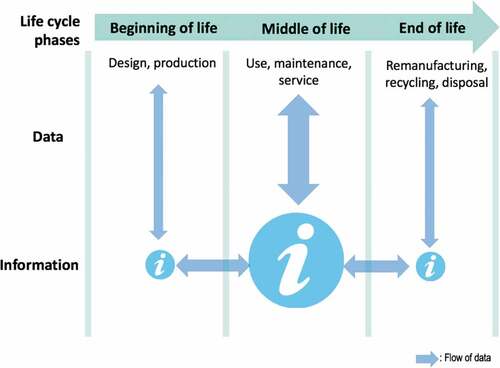
The product lifecycle starts with choices made before manufacturing, e.g. materials and components chosen for a product. Without loss of generality, a typical product such as a car, truck or plane is assumed for this paper. The manufacturer provides regular maintenance and emergency repair services through a maintenance technician during the product lifecycle, usually based on an agreed-upon service contract. This may also contain service level agreements, where acceptable interruptions to using a product are stipulated, and fines for deviations detailed. In the following sections, it is assumed that the use of the product is sold as a service. This means that the manufacturer and customer’s interests align with reducing total lifecycle costs and that the manufacturer has a large degree of control over the product lifecycle. It is also assumed that there are no externalities, such that environmental costs and financial costs are aligned, and decision problems can be reduced to a single objective. Figure 1 shows the product lifecycle. Most of the data come from the MOL stage, e.g. the use phase, which is usually the starting point for coupling with AI. The additional data coming from the BOL and EOL can, in turn, contribute to other lifecycle stages and, eventually, the whole lifecycle for optimal decision-making. This paper demonstrates using AI to optimise decision-making and planning during the use phase of the product lifecycle, i.e. MOL, particularly in operations and maintenance. The idea of using AI in other product lifecycle phases BOL, EOL is all similar. They are all seen as different cases to be tailored with AI solutions. This paper particularly introduces a typical example using AI for maintenance in detail.

Figure 1. AI for product lifecycle management.

4. AI system for decision making and planning focusing on maintenance

This section explores how to apply a selection of general AI techniques for maintenance and sustainability problems. The discussion and case studies are centred around the simplified product lifecycle diagram shown in Figure 2, which arose from discussions with the participating case companies.

Figure 2. The simplified product lifecycle from a maintenance perspective.

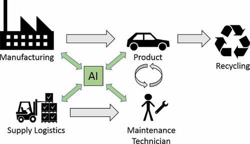
While in Figure 2, AI is illustrated as a central role, in practice, it is more likely that it serves in several separate systems for particular sub-problems. It is important to note that a prerequisite for integrating AI into a traditional product lifecycle requires an adequate information technology infrastructure to collect, store and process relevant data. Whether to situate AI functionality onboard a product or in a centralised location depends on the real-time requirements of the task, the available bandwidth, and the processing power onboard. Centralisation, in theory, can lead to better decision-making by continuously aggregating information across all products and all steps of the lifecycle. For example, knowing the current projected maintenance needs of the fleet aids individual maintenance technicians and the logistics of spare part, inventory management, and product design. Most tasks in maintenance do not have stringent real-time requirements, which suggests a mostly centralised AI is technologically feasible. In this regard, other trends such as Internet-of-things (IoT), big data infrastructure, and cloud computing can be key enablers of AI.

Typical AI techniques such as machine learning attempt to give machines some ability to learn from data instead of being explicitly told and programmed how to handle every situation (Bishop 2006). The discipline is traditionally divided into three types of learning: supervised learning, unsupervised learning and reinforcement learning (RL). Although the techniques used to solve these problems share theoretical foundations with statistics and optimisation, they differ in learning being more focused on data-driven approaches. Data-driven approaches attempt to infer patterns and solve problems with little prior knowledge, viewing the problem more like a ‘black-box’, but this requires sufficient high-quality data to achieve reasonable performance. To be able to model an arbitrarily complex problem, some sufficiently powerful generic model is needed. A popular choice is artificial neural networks, which under mild conditions is a universal approximator. In addition, multi-layer neural networks can learn multiple layers of abstraction under suitable conditions, so-called deep learning (Goodfellow, Bengio, and Courville 2016), which has recently allowed people to tackle larger problem domains than previously possible.

In the following section, the authors identified and developed a taxonomy of different types of problems in maintenance based on discussions with the case companies and how they fit with different AI techniques. As data-driven AI techniques were found to be of most interest, that is where the authors chose to focus.

Based on the discussions with the participating companies and literature studies, the following taxonomy of promising AI applications was identified.

• Modelling failures

  • Diagnostics (what failed)

  • Anomaly detection (has something failed)

  • Prognostics (when will it fail)

• Automatic decision making

  • Planning preventative maintenance (when/what to maintain)

  • Decision support and planning for repair (how to repair)

  • Spare part logistics (inventory costs vs downtime costs)

  • Automatic tuning

4.1 Modelling failures

In many cases, modelling and making inferences from data-driven problems can be reduced to the combination of supervised learning and unsupervised learning. Some domain-specific considerations do apply when it comes to what models to learn and what learning algorithm to use. Black-box models typically require the least amount of work. In particular, deep neural network software tools such as TensorFlow (Abadi et al. 2016) are fairly mature. On the other hand, data on products can be costly to collect, and some prior knowledge may exist, for example, in the form of physics-based models of product behaviour, or at least on the structure of the problem. This suggests using more tailored models, and perhaps even probabilistic inference methods are needed in case of a major data shortage. However, although mature tools also exist for probabilistic modelling (Carpenter et al. 2017), such domain-specific models typically require more work to implement. Determining which approach is the most suitable has to be done on a case-by-case basis, but black-box models provide a good starting point.

The authors leave implementation details and instead focus on the types of problems that could be solved with these techniques. The terminologies of Jardine, Lin, and Banjevic (2006) were used to classify these problems into the broad categories below.

4.1.1 Diagnostics

Diagnostics aims to diagnose suspected or actual failures in a product, such as decision support for the maintenance technician onsite or directly to the customer. Given sufficient examples of past problems and their solutions, bringing this into a machine learning framework as a supervised learning problem is straightforward. Input data x could consist of system measurements, product age, use, type, past service history, etc. The output is the cause of the problem found by the technician. It is then straightforward to learn a model y = f(x) to classify new observed inputs into likely causes.

This is the most straightforward application of machine learning techniques but also the narrowest in scope. By leveraging advances in deep learning, even high-dimensional and semi-structured data such as text, sound or images may be used as inputs. However, depending on the complexity of the model, these may require a large number of examples to learn a useful diagnostic model. Such deep learning is already common in medical diagnosis based on images (Kermany et al. 2018; Litjens et al. 2017), and there are reports of General Electrics using such AI to diagnose jet engine problems from the sound they make (Sina Tayarani-Bathaie, Sadough Vanini, and Khorasani 2014; Woyke 2017).

4.1.2 Anomaly Detection and Monitoring

Anomaly detection attempts to detect anomalies, which can be used to trigger preventive maintenance before a suspected fault. A diagnostics model can also be used pre-emptively for anomaly detection, and it is sometimes sorted under diagnostics in the maintenance literature.

Anomaly detection can also benefit from a different machine learning approach than just relying on manually labelled examples of failures. Since the objective is to detect deviations from some normal system state that fluctuates over time, a self-supervised or unsupervised approach is also applicable. A self-supervised model can be trained to predict a new state based on the preceding values. The prediction can then be compared with the outcome over time and flag large deviations for inspection. Such self-supervised learning has the advantage of not needing manual labelling of failures, so large quantities of data can be collected via other solutions such as IoT devices.

If one suspects there is an important unobserved state in the problem, one can also use unsupervised learning techniques to infer this and do outlier detection on such a ‘hidden’ state instead of directly on measurements.

Such self-supervised and unsupervised anomaly detection techniques cannot offer a diagnosis or even prove that something is wrong. They can, however, serve as a warning indicator that the system behaviour is unusual, which might warrant further inspection.

4.1.3 Prognostics

Prognostics attempts to build models of when a product, or component, will fail. That is, to predict its life span, sometimes called the remaining useful life (RUL) or time to failure (TTF). It, therefore, looks further ahead than the diagnostics models. While often used differently, a sufficiently advanced prognostics model can subsume diagnostics in that one can compute the currently most likely failure from predicted failure times of each part.

While such prognostics models are more powerful than diagnosis models, they are also subtly more complex than a typical supervised learning problem. Typically, life span is only observed indirectly via failures. Such models need to reflect this type of ‘censored’ data unless the product life span is short concerning the data record. An elegant solution is to use a hierarchical probabilistic model, where the life spans can be treated as an internal state to be inferred from observations. This approach has also recently been combined with deep neural networks (Hwang et al. 2019; L. Wang et al. 2017; Guo et al. 2021a). A simpler approach is to split the life span into fixed discrete intervals. As the failures in each fixed-time interval are known, one can compute the failure probability. This sidesteps the problem at the price of some model fidelity. Deep learning for survival analysis was recently surveyed in (Nezhad et al. 2019), which also proposed a particular implementation for time-series event data, which seems promising for sensor data or maintenance history. Several open-source variations on this theme also exist, e.g. (Zhao et al. 2019; Längkvist, Karlsson, and Loutfi 2014; Spacagna 2018).

4.2 AI-assisted decision making

Decision-making is an important topic in maintenance. For example, if a model over failure probabilities exists or is learned using AI techniques, it can be used to optimise the maintenance process. These decision problems can be solved algorithmically and automated via either classical decision techniques or more general AI techniques such as RL. Here are some ideas for using AI to automate and improve decision-making in maintenance problems.

4.2.1 Planning for preventive maintenance

Learned models of time to failure, per part or product, can be used for several maintenance planning problems. Prognostics models that output a probability distribution over failures are ideal for planning maintenance and preventive replacements of parts. A model that can make informed predictions on a per-product basis would also adapt the maintenance on a per-product basis. A failure model over simple discrete time intervals can be used to decide which parts to preventively replace in a maintenance window, while a continuous-time failure model would also allow adapting the maintenance intervals themselves.

There are considerable existing work on maintenance scheduling, e.g. (Froger et al. 2016; Duan et al. 2018; Gustavsson et al. 2014). However, most used simpler predictive models than the proposed one in this paper and fairly specialised solution techniques. In principle, such classical scheduling techniques also carry over to machine-learned models. RL can bring to this problem a general-purpose approach to find approximate solutions even for large decision problems.

As mentioned earlier, diagnostics and anomaly detection can also be used preventively as an indicator of when to involve a maintenance technician. With the growth of IoT, this can also be automated to contact a maintenance technician for a closer look. When to trigger such an inspection or repair action is a decision problem, and an optimal decision policy can likewise be found via, e.g. RL. Since anomaly detection can typically leverage more data, it appears prudent to use a tiered approach with both anomaly detection for early warning and more granular time to failure models for preventive maintenance or replacement of individual parts.

Finally, products or parts become costlier to maintain over time or fall behind new models in energy efficiency or other environmental costs. At some point, it may be optimal to simply recycle the product (or part) and replace it with a new model, illustrated as the final arrow in Figure 2. This is also a decision problem, and as the acquisition cost has to be weighed against discounted future maintenance costs, it is a sequential decision problem suitable for RL.

4.2.2 Decision support and planning for repair

A diagnostic model that directly predicts the problem cause can trivially be used as onsite decision support of which part to replace by a maintenance technician. More advanced use of decision support is if a tailored diagnostic model of the product exists as a Bayesian network, but the cause is unknown yet. Such Bayesian networks can be used to automate the troubleshooting process by automatically creating plans that yield the most information about the cause of the problem in the fewest steps (Cai, Huang, and Xie 2017).

4.2.3 Spare part logistics

Modern logistics is pushing down storage requirements, and when and where to stock parts is crucial for lean inventory management. One promising idea is to use the powerful learned time to failure models to improve predictions. It would even be possible to make per-product predictions to push such logistics to the limit. Decision theory and RL would give a principled way to factor in the risks imposed by downtimes and service level agreements and weigh this against the cost of potentially redundant inventory.

4.2.4 Automatic tuning

Finally, with the growth of IoT, it is easier than ever to collect diagnostic data from fleets, which can be used to learn diagnostic, time to failure and anomaly models collectively. This information can also be leveraged and flow back out to products again. The authors speculate that automatic tuning or self-improvement is a potential future application of AI. Some automakers are already routinely sending out over-the-air software updates. These can adapt parameters that control how a product operates, such as an engine or battery, potentially impacting lifetime, energy efficiency and environmental costs. By leveraging AI, product parameters could automatically be optimised based on their usage profile.

5. Case study based on RL techniques

Based on a broad review of classic AI techniques in connection with the real-world situation and especially the case companies, the authors consider RL most suitable for providing customised decision support for product lifecycle sustainability, considering the case company settings and constraints, including e.g. data availability, data processing capability, stakeholder preferences, etc. Essentially, RL provides an agent with a way to generate a utility function based on its experience executing actions in its environment and observing the results. Unlike the popular deep neural network learning-based approaches that rely on big data to obtain acceptable performance, sufficient and high-quality data is typically absent throughout the lifecycle. This is due to the lack of proper data collection infrastructure, especially with long life-span products, e.g. produced decades ago. For RL, an implicit part of the observation is whether the outcome state is good or bad relative to the agent’s performance metric. The agent can then generate optimal plans that determine the proper action to take in any state. This perfectly suits the situation in which the scarcity and uncertainties of data across the product lifecycle typically exist for companies in real-world reality, including the studied case companies.

This section presents a case study of the application of discrete, tabular, RL techniques in three different maintenance scheduling problems in Company-X. See Appendix A and Appendix B for the detailed adoption of the RL and Markov decision process (MDP) model for this problem.

Company-X is a Swedish manufacturer producing industrial vehicles related products to other companies (Company-Y_i), operators of warehouses, workshops, manufacturing facilities, etc. Company-X also provides maintenance services to its customers as part of rental contracts in PSS mode. One of the products X has a 36-month warranty, and the company is interested in determining a maintenance schedule to maximise profits for the use of Product-X during those 36 months. Either Company-X is interested in selling maintenance as a service or in advising companies (Company-Y_i) in which the product is sold as to a proper maintenance schedule. Since companies use Product-X under different conditions, the maintenance schedules may differ from company to company and even from different Product-X’s purchased by the same company.

Generally, Product-X can be in one of two states at a specific point in time (in this example, t ∈ [0, 35] where t represents one of 36 months):

• Failure(t)

• Good(t)

If Product-X fails in a state, Company-Y can repair it or not. If the product is good in a state, Company-Y can maintain it or not. Each month Product-X functions without failure, Company-Y derives a profit of 10,000 SEK. The cost to repair Product-X on failure is 6,000 SEK. The cost to maintain Product-X in good states is 3,000 SEK.

Suppose either Company-X has collected customer data on maintenance behaviour from individual companies for 36-month periods, or an individual company has collected data about maintenance behaviour for x number of Product-X that they operate. Additionally, they have automatically annotated profit/loss info as rewards. The collected data does not have to be complete, but it is assumed one can ascertain the state of Product-X during each measurement. The annotated rewards are based straightforwardly on the profit, cost to repair and cost to maintain parameters.

Each data point may be viewed as a collection of 4-tuples: (s₀, a₀, r₁, s₁). For the 36-month period, it is assumed that the data collected is represented as an episode consisting of a sequence of 4-tuple measurements associated with the Product-X’s. The size of the sequence is between 1 and 36 data points.

The following provides some examples of episodes:

[’good-6ʹ, ’nm’, 10, ’good-7ʹ, ’nm’, 10, ’good-8ʹ, ’nm’, 10, ’good-9ʹ, ’nm’, 10, ’good-10ʹ, ’m’,

7, ’good-11ʹ, ’nm’, −10, ’fail-12ʹ, ’r’, 4, ’good-13ʹ, ’nm’, −10, ’fail-14ʹ, ’r’, 4, ’good-15ʹ, ’m’, 7,

’good-16ʹ, ’nm’, 10, ’good-17ʹ, ’m’, 7, ’good-18ʹ, ’m’, 7, ’good-19ʹ, ’nm’, −10, ’fail-20ʹ, ’r’, 4,

’good-21ʹ, ’nm’, 10, ’good-22ʹ, ’m’, 7, ’good-23ʹ, ’nm’, 10, ’good-24ʹ, ’nm’, −10, ’fail-25ʹ, ’r’,

4, ’good-26ʹ, ’nm’, −10, ’fail-27ʹ, ’r’, 4, ’good-28ʹ, ’nm’, 10, ’good-29ʹ, ’m’, 7, ’good-30ʹ, ’nm’,

10, ’good-31ʹ, ’nm’, −10, ’fail-32ʹ, ’nr’, −10, ’fail-33ʹ, ’nr’, −10, ’fail-34ʹ, ’nr’, −10, ’fail-35ʹ, ’r’,

4, ’good-36ʹ]

[’good-31ʹ, ’m’, 7, ’good-32ʹ, ’nm’, 10, ’good-33ʹ, ’nm’, −10, ’fail-34ʹ, ’r’, 4, ’good-35ʹ, ’m’, 7, ’good-36ʹ]

[’good-30ʹ, ’nm’, 10, ’good-31ʹ, ’nm’, 10, ’good-32ʹ, ’m’, 7, ’good-33ʹ, ’m’, 7, ’good-34ʹ, ’m’, 7, ’good-35ʹ, ’nm’, −10, ’fail-36ʹ]

[’good-22ʹ, ’m’, 7, ’good-23ʹ, ’nm’, −10, ’fail-24ʹ, ’r’, 4, ’good-25ʹ, ’m’, 7, ’good-26ʹ, ’m’, 7,

’good-27ʹ, ’nm’, 10, ’good-28ʹ, ’nm’, −10, ’fail-29ʹ, ’nr’, −10, ’fail-30ʹ, ’r’, 4, ’good-31ʹ, ’m’, 7, ’good-32ʹ, ’nm’, −10, ’fail-33ʹ, ’nr’, −10, ’fail-34ʹ, ’r’, 4, ’good-35ʹ, ’nm’, −10, ’fail-36ʹ]

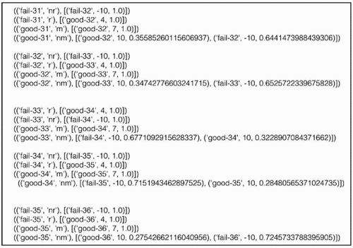
The emphasised 4-tuples provide variations on the type of measurements one can receive:

• ’good-6ʹ, ’nm’, 10, ’good-7ʹ – In month 6, Product-X is in good condition, and no maintenance was done. In month 7, it was still observed to be in good condition, resulting in a profit of 10 (where 10 represents 10,000 SEK).

• ’good-31ʹ, ’m’, 7, ’good-32ʹ – In month 31, Product-X is in good condition and maintenance was done. In month 32, it was still observed to be in good condition, resulting in a profit of 10 − 3 = 7 (where 7 represents 7,000 SEK), and the profit was reduced by 3,000 SEK for the maintenance cost.

• ’good-33ʹ, ’nm’, −10, ’fail-34ʹ – In month 33, Product-X is in good condition, and no maintenance was done. In month 34, it was observed to have failed, resulting in a profit loss of −10 (where −10 represents −10,000 SEK).

• ’fail-24ʹ, ’r’, 4, ’good-25ʹ – In month 24, Product-X is in a failure state and repair was done. In month 25, it is now in good condition, resulting in a profit of 4 (where 10–6 = 4 represents 4,000 SEK), and the profit was reduced by 6,000 SEK for the repair cost.

Figure 3 depicts several different ways to apply RL to this problem.

Figure 3. Some RL scenarios.

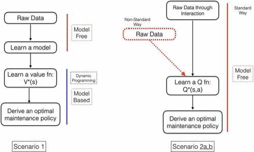
In scenario 1, raw data is used to learn a model, and the learned model is essentially a finite MDP. Dynamic programming techniques can then be applied to the model to generate an optimal policy for the learned model. Note that if the model being learned is non-Markovian, then the resulting Markovian model is only an approximation, and the policy generated is not guaranteed to be optimal, other than being optimal relative to the finite MDP generated.

Scenarios 2a-b use Q-learning, which is a model-free RL approach based on interaction with the environment. In scenario 2b, raw data is gained through interaction with the environment. This can be based on simulation or collecting sensor data interactively. In this case, one can directly collect data about Product-X in operation. This data is used to learn a Q function incrementally similar to a value function on the state but considers the specific actions used to reach states. The Q function is updated per interaction (s_t,a_t,r_t+1, s_t+1). Given a Q function, one can then generate an optimal policy.

In scenario 2a, it is assumed that data has been collected for previous interactions with Product-X and saved in a data repository. One can then use this data and input 4-tuples to the Q-learning algorithm to generate a Q function for the saved data. Scenarios 2a and 2b are similar, but only 2b is truly interactive and learning a Q function through live interaction with a system.

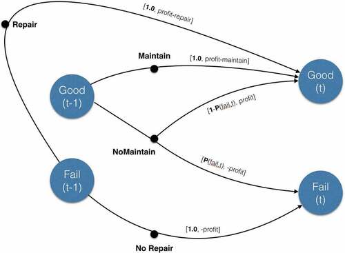
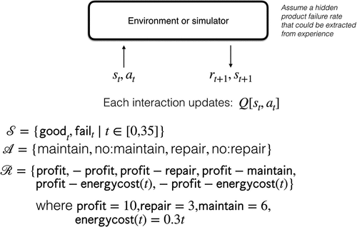
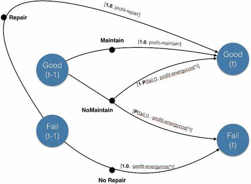
5.1 Example 1: A hidden failure rate for Product-X

In example 1, a simulator is used for Product-X, where the only information that can be derived by an agent is through exploratory interaction with the simulator by entering state-action pairs and recording the reward and next state output from the simulator as a result (see Figure 4). Of course, the idea is to use the actual product and its sensor outputs instead of a simulator which one generally does not have in real-world scenarios.

Figure 4. Example 1: Hidden failure rate for Product-X.

Figure 5 depicts the hidden simulation model used for experiments with example 1. A failed product at time (t-1) will transition to good at time (t) with repair under probability 1 and net profit as profit-repair, or will transition to fail at time (t) without repair under probability 1 and net profit as -profit. Similarly, a good product at time (t-1) will transition to good at time (t) with maintenance under probability 1 and net profit as profit-maintain, or without maintenance under probability 1-P(fail, t) and net profit as profit, or will transition to fail at time (t) without maintenance under probability P(fail, t) and net profit as -profit.

Figure 5. Example 1: the simulation model.

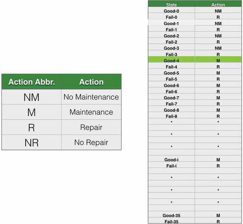
In these experiments, the sample size is set at 100,000 generated episodes. The optimal policy resulting from the application of Q-learning to this scenario is shown in Figure 6. The state column lists the conditions of the product at month [0, 35], and the action column lists the optimal action decisions that should be taken from [no maintenance, maintenance, repair, no repair].

Figure 6. Example 1: optimal policy.

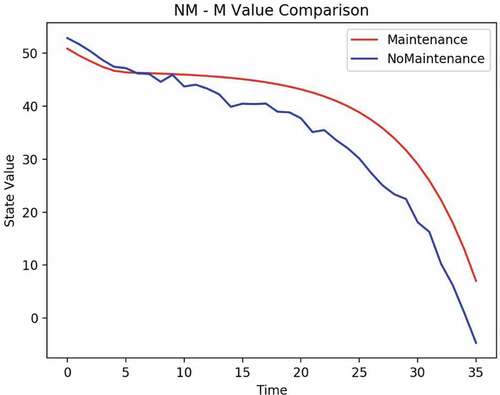
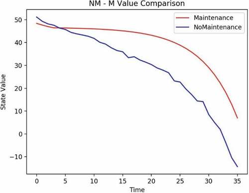
From the Q function, one can determine that the crossover period, as shown in Figure 7, from doing no maintenance to requiring maintenance is in month 6. It means that the optimal action decision should start maintenance from month 6 even if the product is in good condition to achieve maximum accumulated profit.

Figure 7. Example 1: maintenance crossover.

To validate the result for interactive Q-learning, the following methodology is used for the learning phase:

• Do a Q-learning (episode) iteration.

• Generate a (soft) policy from the current Q[s, a] table.

• Run this policy in the validation mode against the simulator (or sensed environment) x times. In this case, x = 400, where 400 episodes are generated.

• Generate the mean average reward for the episodes generated.

• Plot the result as iteration 1 in the graph and repeat for y iterations.

Figure 8 shows the convergence of the Q-learning algorithm for 100,000 iterations. It can be seen that the reward curve is stabilised at around 250, which is in line with the M_R policy curve in Figure 9.

Figure 8. Example 1: reward validation.

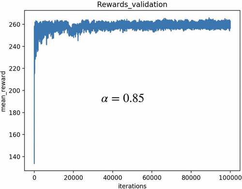
Figure 9. Example 1: mean rewards.

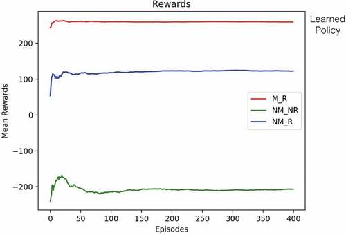
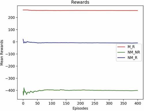
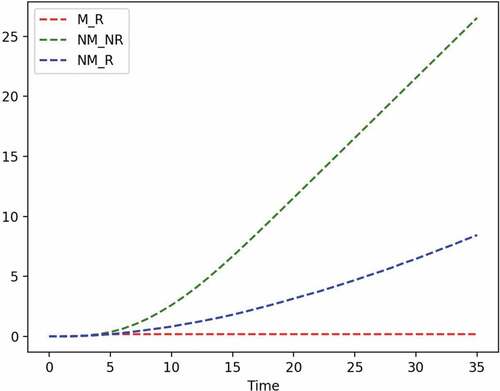
Figure 9 shows a post-learning analysis with three different policies. NM_NR is a policy that never does maintenance and never does repair. If run against a simulator/environment, one can see that the mean average reward for x episodes fluctuates initially but then settles in at a very low rate, around −200, which means loss of profit. NM_R is a policy where no maintenance is done, but the repair is done when the product fails. It does somewhat better in terms of rewards, settling in at around 100. One sees a remarkable improvement in reward for the learned policy M_R output by the Q-learning algorithm, settling in the vicinity of 250.

Mean time to failure (MTTF) is a parameter often used to measure the quality of a product. MTTF measures the average time before the product fails. Figure 10 shows the behaviour of a product using the three different policies, M_R, NM_NR, and NM_R. One thousand samples were used to generate the graph. It shows that for the learned policy, M_R, there is no failure during the 36 months. For the NM_R policy, one sees some degradation and a linear increase in MTTF at each time point after 7 months. For the NM_NR policy, there is a sharp linear increase in the MTTF rate after 5 months.

Figure 10. Example 1: MTTF.

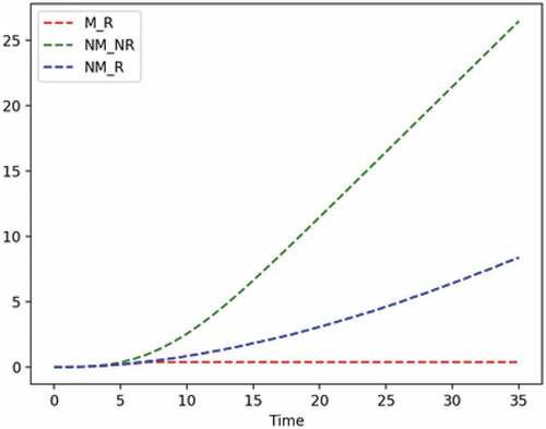
Figure 11. Example 2: hidden failure rate with energy cost.

5.2 Example 2: A hidden failure rate for Product-X with energy cost

In example 2, the same assumptions apply as in example 1. Besides, there is an energy cost when Product-X is not maintained or repaired, and the energy cost increases with time. In states where one transitions from a good state to a good state without maintenance, the reward is profit−energycost(t). In states where one transitions from a good state to a fail state without maintenance, the reward is −profit − energycost(t). When one is in a fail state and transitions to a fail state without repair, the reward is −profit−energycost(t). Otherwise, rewards remain as in example 1 (see Figure 11).

Figure 12 depicts the hidden simulation model used for experiments with example 2. This is similar as explained in Figure 5 but with additional energycost(t) without maintenance or repair.

Figure 12. Example 2: the simulation model.

In these experiments, the sample size is set at 100,000 generated episodes. The optimal policy resulting from the application of Q-learning to this scenario is shown in Figure 13. The state column lists the conditions of the product at month [0, 35], and the action column lists the optimal action decisions that should be taken from [no maintenance, maintenance, repair, no repair].

Figure 13. Example 2: optimal policy.

From the Q function, one can determine that the crossover period, shown in Figure 14, from doing no maintenance to requiring maintenance is in month 4. It means that the optimal action decision should start maintenance from month 4 even if the product is in good condition to achieve maximum accumulated profit.

Figure 14. Example 2: maintenance crossover.

The same validation methodology as used in example 1 is also used for example 2. Figure 15 shows the convergence of the Q-learning algorithm for 100,000 iterations. It can be seen that the reward curve is stabilised at around 250, which is in line with the M_R policy curve in Figure 16.

Figure 15. Example 2: reward validation.

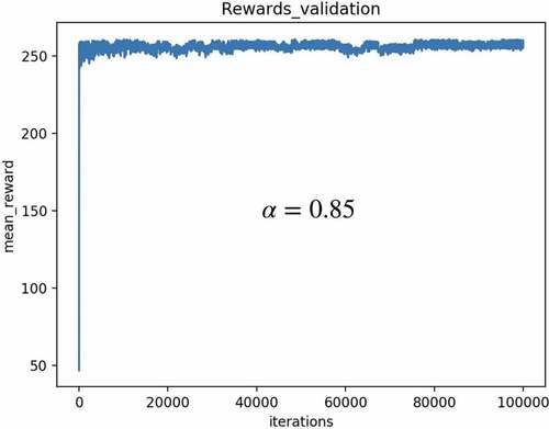
Figure 16. Example 2: mean rewards.

Figure 16 shows a post-learning analysis of the mean reward with three different policies. NM_NR, NM_R, and M_R. Notice there is a significant shift for the NM_NR and NM_R policies where there are profit loss and no profit, respectively.

Figure 17 shows the MTTF behaviour of a product using the three different policies, M_R, NM_NR, and NM_R. One thousand samples were used to generate the graph.

Figure 17. Example 2: MTTF.

5.3 Example 3: Learning a model

For example 3, the same criteria as in example 1 were assumed, with the same hidden failure rate. The goal is to learn a model, an MDP, that supports the raw data generated through interaction with a simulator/environment. The learning scenario 1 discussed earlier in Figure 3 was used.

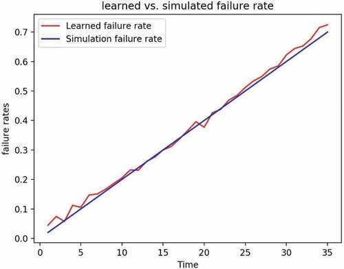
Begin by generating 10,000 episodes through interaction with a simulator/environment to generate 4-tuples (s_t,a_t,r_t+1, s_t+1). Then learn probability distributions for s_t,a_t, pairs, P (S_t+1, R_t+1 | S_t,A_t), by counting frequencies. Recall that from such a probability distribution, one can generate all aspects of a finite MDP. The resulting model is shown in Appendix C.

Given this model, one can use dynamic programming techniques to generate a value function, V * from the model. Using V *, one can then generate an optimal policy for the model. As it turns out, the optimal policy generated is exactly the policy learned in example 1. This is not too surprising since the raw data to learn the model was generated using a simulation model that was the same for interactive Q-learning.

In Figure 18, the learned failure rate is compared with the simulated failure rate. One can see that the learned failure rate is a close fit to the simulated failure rate.

Figure 18. Comparison of learned and simulated failure rate.

5.4 Discussion

5.4.1 The characteristics of RL technique

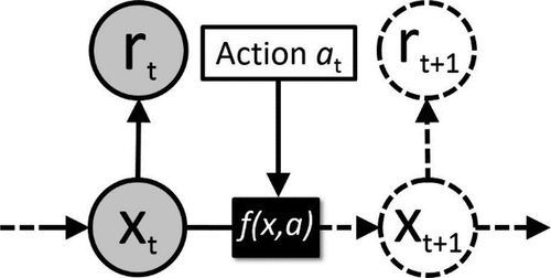
RL extends machine learning beyond just modelling and prediction to also decision-making. The algorithm is a rational agent that learns how to act in an uncertain environment by trial and error. The agent need only be given the problem state at the current time x_t and the immediate reward r_t of that state. The reward can be seen as the profit of a business decision, or equivalently the inverse cost, material and environmental. Such profits and costs are condensed into one number, the reward, which the agent uses as feedback on improving. As seen in Figure 19, at each step, the agent will have to select an action a_t, which will result in a new problem state and a new reward. This is a sequential decision problem as the sequence of actions determines the resulting sequence of states and rewards. The agent will have to plan a number of steps into the future to find the sequence of actions that maximises the total reward over time. In classic RL, no prior knowledge is needed of either the rewards or how the problem state changes in response to an action, x_t+1 = f (x_t, a).

Figure 19. RL extends learning to simultaneously solving a decision problem. Given just a problem state x_t and a reward for that state r_t, the agent will try to learn how to maximise the profits or minimise the costs over time. This can be visualised as a Bayesian network augmented with action nodes, where at each point in time t it has to make a decision based on the history of observed states and rewards.

RL provides a way of learning behaviour that does not rely on being provided with correct examples. In many real-world cases, the rewards and costs of the problem states are known and easy to define, and therefore such algorithms can learn autonomously, either in simulation or directly in the target environment. Since they encompass both learning and planning, such algorithms appear naturally suited for use cases in robotics and autonomy. As RL is applicable to any decision-making task under uncertainty, it has also found uses outside robotics and simulated worlds. For example, in a wide variety of operations research problems like inventory management and scheduling (Powell and Topaloglu 2006), considerable uncertainty and approximations may be needed as exact solution techniques are infeasible to compute. As many real-world business problems fall in this category, RL can be seen as a promising avenue for approaching complex sequential business decisions.

5.4.2 Application considerations

Real-world companies, including the studied case companies, need a robust method to handle situations with the scarcity and uncertainties of data across the product lifecycle to support decision-making. While machine learning may appear like a silver bullet, the key limitation of learning approaches is the availability of large and useful data sets for the task at hand. This can be a bottleneck in many traditional industrial and manufacturing sectors where margins are small, and collecting data can require investment in sensors, coordination with customers and infrastructures. Secondary bottlenecks of machine learning include computational requirements, primarily to train these models from data, but potentially also to use them for making new predictions.

Common off-the-shelf techniques for black-box models work best when there is ample useful data available, and either there is a moderate number of relevant input variables, or the complexity of the problem is low. If there is a great number of relevant input variables, off-the-shelf tools for black-box models may scale poorly. However, for problem domains with an inherent hierarchical structure such as text, image and speech, deep learning techniques can leverage large data sets and GPU hardware to overcome this limitation. In, e.g., image classification tasks, input images may contain 1 million pixel values, and deep learning techniques have come to dominate the field, but decision-making is far from that.

Problems with a small amount of data in relation to the number of variables remain a problem. It is also not uncommon for a seemingly large data set to contain a series of small-data problems. In these cases, one can benefit from including prior knowledge about the task one is trying to learn either directly on parameter values or the structure of the problem. Probabilistic approaches are the most theoretically sound framework for incorporating such prior knowledge (Bishop 2006; Gelman et al. 2013), where they can intuitively be visualised as inference in a Bayesian network, structured after the task at hand. A significant advantage of probabilistic learning is that it considers the level of confidence in the learned model and allows easier introspection of the results. However, such Bayesian learning techniques can be too computationally intensive, and probabilistic models therefore often require tailored solutions.

Using machine learning to learn a model of some business problem is often to improve decision-making. Initially, as decision support for manual decision-making, these could also be automated via, e.g. RL techniques. Another common use case is anomaly detection, automatically finding and flagging ‘outliers’, data points that may represent abnormal behaviour. Once these have been identified, domain experts can examine them to figure out what, if anything, is wrong. For example, an identified anomaly in component longevity may be detected in a manufacturing process to examine the underlying cause. As most off-the-shelf machine learning tools focus more on mean-value predictions, being right on average rather than rare occurrences, accurate anomaly detection may require more tailored probabilistic approaches. In summary, RL is suitable and appropriate for the decision-making problem defined in the context of this paper.

6. Conclusions

In this study, the authors proposed using AI to optimise decision-making and planning based on historical and real-time data and human expert knowledge. The application of AI is investigated for decision-making and planning towards sustainable operations in product lifecycle phases. RL is adopted as the most suitable AI technique RL for the optimal decision-making purpose, which is validated through a real industry case. Firstly, the key stages are identified in which AI can support decision-making across the product lifecycle. Then, typical cases and a generalised method and procedure are proposed with AI for decision support based on lifecycle data (such as data obtained from operations and maintenance) to improve sustainability. An illustrative case study, combining with modelling and simulation, is conducted to demonstrate the feasibility and performance of the proposed method using AI to improve the decision-making and planning in the MOL stage. The proposed method can achieve optimal decision policy to achieve maximum accumulated profit.

The main contributions of this paper over the existing works are 1) The data came from real industry, and the proposed method was empirically applied with action research. 2) The AI-based decision process covered a wider lifecycle stage. 3) It contributed to sustainability goals, particularly prolonging the product lifetime and reducing environmental impact. In summary, this paper enriches the knowledge of using AI techniques to optimise decision-making and planning for achieving optimal sustainability throughout the product lifecycle.

The limitation of the current study is that it mainly focuses on the MOL phase, and the optimisation is designed for each lifecycle phase. In future research, the optimisation will be expanded to cover the entire lifecycle phases. It will combine data and knowledge obtained and derived by AI from all lifecycle phases to further enhance the optimisation towards sustainability.

Acknowledgments

A part of this paper (mainly the case study and the appendix) is based on excerpts from an unpublished internal report authored by P. Doherty, O. Andersson and J. Kvarnström (Linköping University), as part of the Vinnova project stated in the funding.

Disclosure statement

No potential conflict of interest was reported by the author(s).

Correction Statement

This article has been republished with minor changes. These changes do not impact the academic content of the article.

Additional information

Funding

This work was supported by the Vinnova [2017-01649].

Appendices

Appendix A. RL and maintenance scheduling

A major topic in the area of sustainability and maintenance is sustainable maintenance scheduling. RL is used as a promising AI technique and is particularly good for dealing with uncertainties and data scarcity, and probabilistic, model-based approaches to RL enable reducing the negative effects of model errors (Deisenroth, Fox, and Rasmussen 2015). Given a product or product component, maintenance scheduling can be influenced by many factors such as profit, cost to maintain, cost to repair, energy costs, degrading health conditions, etc. This case study and associated experiments are intended to provide a conceptual landscape for how (tabular) RL can be used in this context. A subset of the experimental ideas considered is loosely based on a related paper by Knowles, Baglee, and Wermter (2011), in which they study maintenance planning. This overview is based on the seminal book by Sutton and Barto (2018) and re-paraphrased. Figure A.1 provides the basic idea behind RL.

Figure A1. RL overview.

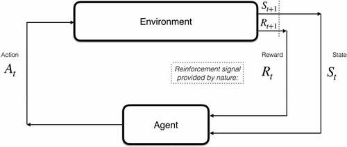
An agent and its environment interact at each of a sequence of (discrete) time steps, t = 0, 1, 2, 3, … This results in a trajectory of state S, action A, and reward R, e.g. S₀, A₀, R₁, S₁, A₁, R₂, S₂, A₂, R₃, … The goal of an agent should be to learn an optimal policy, from its experience while interacting with the environment, that determines which action to execute in each state to maximise its accumulated rewards. The reinforcement signal or reward is assumed to be provided by nature or the environment in question. For instance, sensor streams of data from a product could characterise the environment, where the product state is summarised, and the reward, positive or negative, is associated with the product’s health status.

There are four major elements in an RL system:

• Policy – provides a behavioural specification of what an agent should do at each state.

  • A policy is a state to action mapping that can be deterministic or stochastic.

• Reward signal – defines the goal in an RL problem.

  • A reward signal determines the immediate, intrinsic value of a state.

  • Rewards determine good and bad events, and nature determines rewards.

  • Rewards are, in general, stochastic functions of the state of an environment and the actions taken.

  • The objective of an agent is to maximise the total reward it receives over the long run based on its interactions with the environment.

  • Agent goals are specified declaratively through the specification of direct rewards for states in the learning domain.

• Value function – specifies what is good in the long run for the agent in terms of states.

  • The value of a state is the total amount of reward an agent can expect to accumulate over the future, starting from an initial state.

  • Actions are then made based on value judgements about the state.

  • RL is, in large part, about value estimation and efficient ways in which it can be determined based on interaction with the environment.

  • Once one has a value function, either stochastic or deterministic, one can determine an optimal policy.

• Model – models mimic the behaviour of an environment and allow agents to infer their behaviour.

  • Model-based reinforcement methods assume a model and use it to determine optimal policies. Consequently, it is a form of planning.

  • Model-free reinforcement methods use trial and error interaction in an attempt to learn models. Once such models are learned, model-based methods can be used to generate optimal policies.

RL is related to several other AI techniques, such as AI search and planning. Model-based methods such as value or policy iteration use dynamic programming are the basis for generating optimal policies. These policies can be viewed as universal plans in the automated planning research area, where the search is used to generate plans in various ways. Essentially, dynamic programming does a breadth-first search on an inverse search graph to generate cost-to-goal measures for each state in the search tree, where each leaf is a policy. The cost-to-goal measures are, in fact, components in a value function. According to Poole and Mackworth (2017), dynamic programming is useful when:

• Goal nodes are explicit. General AI search and planning can use functions to recognise goal states.

• The lowest cost path is needed.

• The graph is finite and small enough to use a table to store cost-to-goal measures for each state.

• The goals do not change very often (since dynamic programming is a form of compilation for a single goal).

• The generated policy is used many times, so the cost of generating an explicit table can be amortised.

There are several problems with dynamic programming:

• The technique only works when the graph is finite, and the cost-to-goal table is small enough to fit into memory.

• An agent would have to re-compute a policy for each different goal.

• The time and space required are linear in the size of the graph, where the graph size for finite graphs is typically exponential in the path length.

Automated planning and search require explicit models, as do tabular-based RL methods. On the other hand, the search graph does not have to be finite, as goal specification is much more generic, and general-purpose planners can easily be reused for diverse goals.

Appendix B.

Finite Markov decision processes (MDPs)

Finite Markov decision processes (MDPs) offer an elegant mathematical model of the RL problem. An MDP consists of:

1. i. S – a finite set of states.

2. ii. A – a finite set of actions.

3. iii. R – a finite set of rewards.

4. iv. A(s) – a specification of applicable actions for each state.

5. S_t,R_t – a set of discrete random variables for each timepoint with probability distributions dependent only on the previous state and action.

For particular values of S_t ∈ S, R_t ∈ R, there is a probability of these values occurring at time t, given particular values of the previous state and action:

$\mathrm{\forall }s{ }^{\mathrm{\prime }},s\in S,r\in R,a\in A,$

(B1) $p(s{ }^{\mathrm{\prime }},r|s,a)\dot{=}Pr\{S_t=s{ }^{\mathrm{\prime }},R_t=r|S_{t-1}=s,A_{t-1}=a\}$(B1)

where p is a deterministic function of four arguments that specifies the probability distribution for each choice of s and a:

(B2) $\sum _{s{ }^{\mathrm{\prime }}\in S}\sum _{r\in R}p(s{ }^{\mathrm{\prime }},r|s,a)=1,\mathrm{\forall }s\in \mathrm{S},a\in \mathrm{A}$(B2)

The dynamics of an MDP is completely characterised by the function p. State-transition probabilities are defined in terms of p as:

p: S × S × A → [0, 1], where,

(B3) $p(s{ }^{\mathrm{\prime }},r|s,a)\dot{=}Pr\{S_t=s{ }^{\mathrm{\prime }}|S_{t-1}=s,A_{t-1}=a\}=\sum _{r\in R}p(s{ }^{\mathrm{\prime }},r|s,a)$(B3)

Expected rewards for state-action pairs are defined in terms of p as:

p: S × A → ℝ, where,

(B4) $r\left(s,a\right)\dot{=}\mathbb{E}[R_t|S_{t-1}=s,A_{t-1}=a]=\sum _{r\in R}r\sum _{s{ }^{\mathrm{\prime }}\in S}p(s{ }^{\mathrm{\prime }},r|s,a)$(B4)

Expected rewards for state-action-state tuples are defined in terms of p as:

p: S × A × S → ℝ, where,

(B5) $r\left(s,a,s^{\prime }\right)\dot{=}\mathbb{E}[R_t|S_{t-1}=s,A_{t-1}=a,S_{t-1}=s^{\prime }]=\sum _{r\in R}r\frac{p(s{ }^{\mathrm{\prime }},r|s,a)}{p(s{ }^{\mathrm{\prime }}|s,a)}$(B5)

The Q-learning algorithm is a temporal difference algorithm. For each interaction with the environment, it updates the Q function using the following update equation:

(B6) $Q\left[s_t,a_t\right]=Q\left[s_t,a_t\right]+\alpha \ast [r_{t+1}+\gamma \ast \underset{a\in A\left(s_{t+1}\right)}{max}Q\left[s_{t+1},a\right]-Q\left[s_t,a_t\right]]$(B6)

The parameter γ takes a value in the interval [0, 1] and is a discount rate that determines how much weight should be placed on future rewards compared to more recent rewards. γ = 0 is a completely greedy algorithm taking no account of future rewards, and γ = 1 takes account of all future rewards but only works in the case where episodes terminate in a finite number of steps.

The parameter α takes a value in the interval [0, 1] and determines the learning rate of the algorithm. Usually, this parameter must be determined empirically. For the experiments, α = 0.85, a constant rate was used. Generally, variable-rate parameterisation is used. The value of both parameters may not be stationary but is often a function of state counts or time.

Figure B.1 provides a sketch of the Q-learning algorithm used in the experiments with direct interaction through simulation or sensing.

The function call update_Q(Q,state0,action0,reward1,state1) uses the update equation (A6).

Figure B1. Q-Learning using interaction.

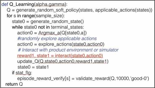
Figure B.2 provides a sketch of the Q-learning algorithm used in the experiments that iterate on raw data episodes provided to the algorithm.

The function call update_Q(Q,state0,action0,reward1,state1) uses the update equation (6).

Figure B2. Q-Learning using raw data.

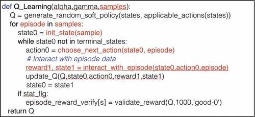
Appendix C.

MDP model depicting the 36 months

Figure C1. Months 0–9.

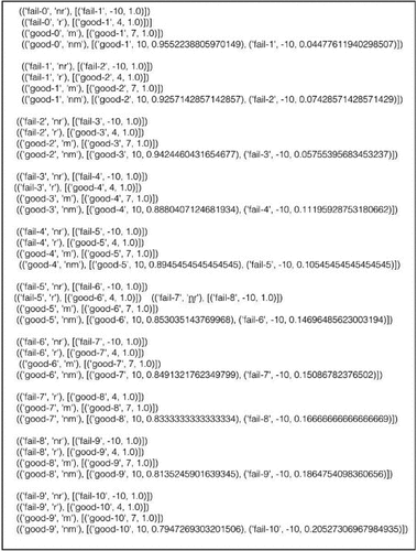
Figure C2. Months 10–19.

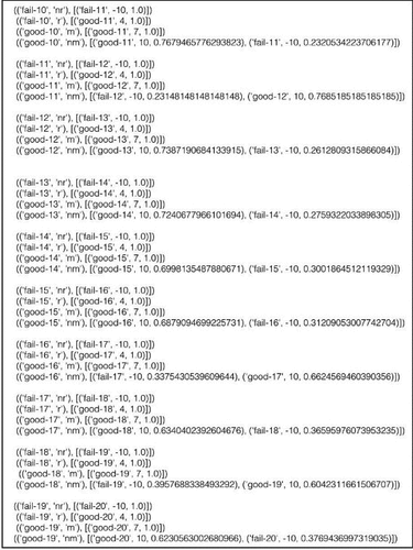
Figure C3. Months 20–29.

Figure C4. Months 30–35.

References

- Abadi, M., P. Barham, J. Chen, Z. Chen, A. Davis, J. Dean, M. Devin, et al. 2016. “TensorFlow: A System for Large-Scale Machine Learning.” In Proceedings of the 12th USENIX Conference on Operating Systems Design and Implementation, 265–283. OSDI’16. USA: USENIX Association.
- Andriotis, C. P., and K. G. Papakonstantinou. 2020. “Deep Reinforcement Learning Driven Inspection and Maintenance Planning under Incomplete Information and Constraints.” ArXiv, July. arXiv. http://arxiv.org/abs/2007.01380.
- Badurdeen, F., R. Aydin, and A. Brown. November 2018. “A Multiple Lifecycle-Based Approach to Sustainable Product Configuration Design.” Journal of Cleaner Production 200: 756–769. Elsevier Ltd. 10.1016/j.jclepro.2018.07.317.
- Bishop, C. M. 2006 Pattern Recognition and Machine Learning. New York: Springer.
- Bosch-Mauchand, M., F. Belkadi, M. Bricogne, and B. Eynard. 2013. “Knowledge-Based Assessment of Manufacturing Process Performance: Integration of Product Lifecycle Management and Value-Chain Simulation Approaches.” International Journal of Computer Integrated Manufacturing 26 (5): 453–473. doi:10.1080/0951192X.2012.731611. Taylor and Francis Ltd.
- Cai, B., L. Huang, and M. Xie. 2017. “Bayesian Networks in Fault Diagnosis.“ IEEE Transactions on Industrial Informatics 13 ( 5): 2227–2240. doi:10.1109/TII.2017.2695583.
- Cai, H., L. D. Xu, B. Xu, C. Xie, S. Qin, and L. Jiang. 2014. “IoT-Based Configurable Information Service Platform for Product Lifecycle Management.” IEEE Transactions on Industrial Informatics 10 (2): 1558–1567. doi:10.1109/TII.2014.2306391.
- Carpenter, B., A. Gelman, M. D. Hoffman, D. Lee, B. Goodrich, M. Betancourt, M. Brubaker, J. Guo, P. Li, and A. Riddell. 2017. “Stan: A Probabilistic Programming Language.” Journal of Statistical Software 76 (1): 1–32. doi:10.18637/jss.v076.i01.
- Deisenroth, M. P., D. Fox, and C. E. Rasmussen. 2015. “Gaussian Processes for Data-Efficient Learning in Robotics and Control.“ IEEE Transactions on Pattern Analysis and Machine Intelligence 37 ( 2): 408–423. doi:10.1109/TPAMI.2013.218.
- Ding, R. X., I. Palomares, X. Wang, G. R. Yang, B. Liu, Y. Dong, E. Herrera-Viedma, and F. Herrera. July 2020. “Large-Scale Decision Making: Characterisation, Taxonomy, Challenges and Future Directions from an Artificial Intelligence and Applications Perspective.” Information Fusion 59: 84–102. Elsevier BV. 10.1016/j.inffus.2020.01.006.
- Duan, C., C. Deng, A. Gharaei, J. Wu, and B. Wang. 2018. “Selective Maintenance Scheduling under Stochastic Maintenance Quality with Multiple Maintenance Actions.” International Journal of Production Research 56 (23): 7160–7178. doi:10.1080/00207543.2018.1436789. Taylor and Francis Ltd.
- Duan, Y., J. S. Edwards, and Y. K. Dwivedi. 2019. “Artificial Intelligence for Decision Making in the Era of Big Data – Evolution, Challenges and Research Agenda.” International Journal of Information Management 48 (October): 63–71. doi:10.1016/j.ijinfomgt.2019.01.021. Elsevier Ltd.
- Ferreira, F., J. Faria, A. Azevedo, and L. A. Marques. 2017. “Product Lifecycle Management in Knowledge Intensive Collaborative Environments: An Application to Automotive Industry.” International Journal of Information Management 37 (1): 1474–1487. doi:10.1016/j.ijinfomgt.2016.05.006. Elsevier Ltd: 1474–1487.
- Froger, A., M. Gendreau, J. E. Mendoza, É. Pinson, and M. L. Rousseau. 2016. “Maintenance Scheduling in the Electricity Industry: A Literature Review.” European Journal of Operational Research 251 (3): 695–706. doi:10.1016/j.ejor.2015.08.045. Elsevier B.V.
- Gao, J. X., H. Aziz, P. G. Maropoulos, and W. M. Cheung. 2003. “Application of Product Data Management Technologies for Enterprise Integration.” International Journal of Computer Integrated Manufacturing 16 (7–8): 7–8. doi:10.1080/0951192031000115813. Taylor & Francis Group: 491–500.
- Geissinger, A., C. Laurell, C. Öberg, and C. Sandström. January 2019. “How Sustainable Is the Sharing Economy? on the Sustainability Connotations of Sharing Economy Platforms.” Journal of Cleaner Production 206: 419–429. Elsevier Ltd. 10.1016/j.jclepro.2018.09.196.
- Gelman, A., J. B. Carlin, H. S. Stern, D. B. Dunson, A. Vehtari, and D. B. Rubin. 2013. Bayesian Data Analysis, 3rd Edition. 675. New York: Chapman and Hall/CRC.
- Goodfellow, I., Y. Bengio, and A. Courville. 2016. Deep Learning. Cambridge, Massachusetts: MIT Press. http://www.deeplearningbook.org
- Govindan, K., A. Jafarian, and V. Nourbakhsh. October 2019. “Designing A Sustainable Supply Chain Network Integrated with Vehicle Routing: A Comparison of Hybrid Swarm Intelligence Metaheuristics.” Computers & Operations Research 110: 220–235. Pergamon. 10.1016/J.COR.2018.11.013.
- Guo, Z., Y. Zhang, J. Lv, Y. Liu, and Y. Liu. 2021a. “An Online Learning Collaborative Method for Traffic Forecasting and Routing Optimization.“ IEEE Transactions on Intelligent Transportation Systems 22 ( 10): 6634–6645. doi: 10.1109/TITS.2020.2986158.
- Guo, Z., Y. Zhang, X. Zhao, and X. Song. 2021b. “CPS-Based Self-Adaptive Collaborative Control for Smart Production-Logistics Systems.“ IEEE Transactions on Cybernetics 51 ( 1): 188–198. doi:10.1109/TCYB.2020.2964301.
- Gustavsson, E., M. Patriksson, A. B. Strömberg, A. Wojciechowski, and M. Önnheim. 2014. “Preventive Maintenance Scheduling of Multi-Component Systems with Interval Costs.” Computers and Industrial Engineering 76 (October): 390–400. doi:10.1016/j.cie.2014.02.009. Elsevier Ltd.
- Hatim, Q. Y., C. Saldana, G. Shao, D. B. Kim, K. C. Morris, P. Witherell, S. Rachuri, and S. Kumara. 2020. “A Decision Support Methodology for Integrated Machining Process and Operation Plans for Sustainability and Productivity Assessment.” The International Journal of Advanced Manufacturing Technology 107 (7): 3207–3230. 10.1007/S00170-019-04268-Y.
- Hwang, H. T., S. H. Lee, H. G. Chi, N. K. Kang, H. B. Kong, J. Lu, and H. Ohk. 2019. “An Evaluation Methodology for 3D Deep Neural Networks Using Visualization in 3D Data Classification.” Journal of Mechanical Science and Technology 33 (3): 3. doi:10.1007/s12206-019-0233-1. Korean Society of Mechanical Engineers: 1333–1339.
- Jardine, A. K. S., D. Lin, and D. Banjevic. 2006. “A Review on Machinery Diagnostics and Prognostics Implementing Condition-Based Maintenance.” Mechanical Systems and Signal Processing 20 (7): 1483–1510. doi:10.1016/j.ymssp.2005.09.012.
- Jarrahi, M. H. 2018. “Artificial Intelligence and the Future of Work: Human-AI Symbiosis in Organizational Decision Making.” Business Horizons 61 (4): 577–586. doi:10.1016/J.BUSHOR.2018.03.007. Elsevier.
- Kaewunruen, S., and Q. Lian. August 2019. “Digital Twin Aided Sustainability-Based Lifecycle Management for Railway Turnout Systems.” Journal of Cleaner Production 228: 1537–1551. Elsevier Ltd. 10.1016/j.jclepro.2019.04.156.
- Kermany, D. S., M. Goldbaum, W. Cai, C. C. S. Valentim, H. Liang, S. L. Baxter, A. McKeown, et al. 2018. “Identifying Medical Diagnoses and Treatable Diseases by Image-Based Deep Learning.” Cell 172 (5): 1122–1131.e9. doi:10.1016/j.cell.2018.02.010. Cell Press.
- Kiritsis, D., A. Bufardi, and P. Xirouchakis. 2003. “Research Issues on Product Lifecycle Management and Information Tracking Using Smart Embedded Systems.” Advanced Engineering Informatics 17 (3–4): 3–4. doi:10.1016/j.aei.2004.09.005. Elsevier BV: 189–202.
- Knowles, M., D. Baglee, and S. Wermter. 2011. In Reinforcement Learning for Scheduling of Maintenance, edited by Bramer, M., Petridis, M., and Hopgood, A. Research and Development in Intelligent Systems, Vol. XXVII, 409–422. London: Springer. doi:10.1007/978-0-85729-130-1_31.
- Längkvist, M., L. Karlsson, and A. Loutfi. 2014. “A Review of Unsupervised Feature Learning and Deep Learning for Time-Series Modeling.” Pattern Recognition Letters 42 (1): 11–24. doi:10.1016/j.patrec.2014.01.008. North-Holland.
- Lee, S. G., Y. S. Ma, G. L. Thimm, and J. Verstraeten. 2008. “Product Lifecycle Management in Aviation Maintenance, Repair and Overhaul.” Computers in Industry 59 (2–3): 2–3. doi:10.1016/j.compind.2007.06.022. Elsevier: 296–303.
- Li, B. H., B. C. Hou, W. T. Yu, X. B. Lu, and C. W. Yang. 2017. “Applications of Artificial Intelligence in Intelligent Manufacturing: A Review.” Frontiers of Information Technology and Electronic Engineering. Zhejiang University. doi:10.1631/FITEE.1601885.
- Li, J., F. Tao, Y. Cheng, and L. Zhao. 2015. “Big Data in Product Lifecycle Management.” The International Journal of Advanced Manufacturing Technology 81: 667–684. doi:10.1007/s00170-015-7151-x. .
- Li, Z., S. Zhong, and L. Lin. 2019. “An Aero-Engine Life-Cycle Maintenance Policy Optimization Algorithm: Reinforcement Learning Approach.” Chinese Journal of Aeronautics 32 (9): 2133–2150. doi:10.1016/j.cja.2019.07.003. Chinese Journal of Aeronautics.
- Lim, K. Y. H., P. Zheng, and C. H. Chen. 2020. “A State-of-the-Art Survey of Digital Twin: Techniques, Engineering Product Lifecycle Management and Business Innovation Perspectives.” Journal of Intelligent Manufacturing 31 (6): 1313–1337. doi:10.1007/s10845-019-01512-w.
- Litjens, G., T. Kooi, B. Ehteshami Bejnordi, A. A. A. Setio, F. Ciompi, M. Ghafoorian, J. A. W. M. van der Laak, B. van Ginneken, and C. I. Sánchez. 2017. “A Survey on Deep Learning in Medical Image Analysis.” Medical Image Analysis 42: 60–88. doi:10.1016/j.media.2017.07.005.
- Liu, X. L., W. M. Wang, H. Guo, A. V. Barenji, Z. Li, and G. Q. Huang. June 2020a. “Industrial Blockchain Based Framework for Product Lifecycle Management in Industry 4.0.” Robotics and Computer-Integrated Manufacturing 63: 101897. Elsevier Ltd: 101897. 10.1016/j.rcim.2019.101897.
- Liu, Y., Y. Zhang, S. Ren, M. Yang, Y. Wang, and D. Huisingh. March 2020b. “How Can Smart Technologies Contribute to Sustainable Product Lifecycle Management?” Journal of Cleaner Production 249: 119423. Elsevier Ltd. 10.1016/j.jclepro.2019.119423.
- Lou, S., Y. Feng, H. Zheng, Y. Gao, and J. Tan. 2018. “Data-Driven Customer Requirements Discernment in the Product Lifecycle Management via Intuitionistic Fuzzy Sets and Electroencephalogram.” Journal of Intelligent Manufacturing 31 (7): 1–16. doi:10.1007/s10845-018-1395-x. Springer New York LLC.
- Ma, Y., K. Rong, D. Mangalagiu, T. F. Thornton, and D. Zhu. July 2018. “Co-Evolution between Urban Sustainability and Business Ecosystem Innovation: Evidence from the Sharing Mobility Sector in Shanghai.” Journal of Cleaner Production 188: 942–953. Elsevier Ltd. 10.1016/j.jclepro.2018.03.323.
- MacCarthy, B. L., and R. C. Pasley. 2021. “Group Decision Support for Product Lifecycle Management.” International Journal of Production Research 59 (16): 5050–5067. June. Taylor and Francis Ltd. doi:10.1080/00207543.2020.1779372.
- Matsokis, A., and D. Kiritsis. 2010. “An Ontology-Based Approach for Product Lifecycle Management.” Computers in Industry 61 (8): 787–797. doi:10.1016/J.COMPIND.2010.05.007. Elsevier.
- Meng, K., Y. Cao, X. Peng, V. Prybutok, and K. Youcef-Toumi. November 2020. “Smart Recovery Decision Making for End-of-Life Products in the Context of Ubiquitous Information and Computational Intelligence.” Journal of Cleaner Production 272: 122804. Elsevier. 10.1016/J.JCLEPRO.2020.122804.
- Nezhad, M. Z., N. Sadati, K. Yang, and D. Zhu. January 2019. “A Deep Active Survival Analysis Approach for Precision Treatment Recommendations: Application of Prostate Cancer.” Expert Systems with Applications 115: 16–26. Elsevier Ltd. 10.1016/j.eswa.2018.07.070.
- Nishant, R., M. Kennedy, and J. Corbett. August 2020. “Artificial Intelligence for Sustainability: Challenges, Opportunities, and a Research Agenda.” International Journal of Information Management 53: 102104. Pergamon: 102104. 10.1016/J.IJINFOMGT.2020.102104.
- O’Leary, D. E. 2013. “Artificial Intelligence and Big Data.” IEEE Intelligent Systems 28 (2): 96–99. doi:10.1109/MIS.2013.39.
- Pomerol, J. C. 1997. “Artificial Intelligence and Human Decision Making.” European Journal of Operational Research 99 (1): 3–25. doi:10.1016/S0377-2217(96)00378-5. Elsevier.
- Poole, D. L., and A. K. Mackworth. 2017. Artificial Intelligence: Foundations of Computational Agents. 2nd ed. Cambridge: Cambridge University Press.
- Powell, W. B., and H. Topaloglu. 2006. Approximate Dynamic Programming for Large-Scale Resource Allocation Problems Models, Methods, and Applications for Innovative Decision Making (Informs)doi:10.1287/educ.1063.0027
- Ren, S., Y. Zhang, Y. Liu, T. Sakao, D. Huisingh, and C. M. V. B. Almeida. 2019. “A Comprehensive Review of Big Data Analytics Throughout Product Lifecycle to Support Sustainable Smart Manufacturing: A Framework, Challenges and Future Research Directions.” Journal of Cleaner Production 210 ( February). Elsevier Ltd: 1343–1365. doi:10.1016/j.jclepro.2018.11.025.
- Rifkin, J. 2000. The Age of Access: The New Culture of Hypercapitalism, Where All of Life Is a Paid-For Experience. New York: JP Tarcher/Putnam.
- Rondini, A., F. Tornese, M. G. Gnoni, G. Pezzotta, and R. Pinto. 2017. “Hybrid Simulation Modelling as A Supporting Tool for Sustainable Product Service Systems: A Critical Analysis.” International Journal of Production Research 55 (23): 6932–6945. doi:10.1080/00207543.2017.1330569. Taylor and Francis Ltd.
- Sina Tayarani-Bathaie, S., Z. N. Sadough Vanini, and K. Khorasani. February 2014. “Dynamic Neural Network-Based Fault Diagnosis of Gas Turbine Engines.” Neurocomputing 125: 153–165. Elsevier. 10.1016/j.neucom.2012.06.050.
- Spacagna, G. 2018. “Deep Time-to-Failure: Survival Analysis and Time-to-Failure Predictive Modeling Using Weibull Distributions and Recurrent Neural Networks in Keras.”
- Sutton, R. S., and A. G. Barto. 2018. Reinforcement Learning, Second Edition: An Introduction. Cambridge, Massachusetts: MIT press.
- Talhi, A., V. Fortineau, J. C. Huet, and S. Lamouri. 2019. “Ontology for Cloud Manufacturing Based Product Lifecycle Management.” Journal of Intelligent Manufacturing 30 (5): 2171–2192. doi:10.1007/s10845-017-1376-5. Springer New York LLC.
- Tao, F., J. Cheng, Q. Qi, M. Zhang, H. Zhang, and F. Sui. 2018. “Digital Twin-Driven Product Design, Manufacturing and Service with Big Data.” The International Journal of Advanced Manufacturing Technology 94: 3563–3576. doi:10.1007/s00170-017-0233-1.
- Wang, L., Z. Zhang, H. Long, X. Jia, and R. Liu. 2017. “Wind Turbine Gearbox Failure Identification with Deep Neural Networks.“ IEEE Transactions on Industrial Informatics 13 (3): 1360–1368. doi:10.1109/TII.2016.2607179.
- Wang, N., S. Ren, Y. Liu, M. Yang, J. Wang, and D. Huisingh. August 2020. “An Active Preventive Maintenance Approach of Complex Equipment Based on a Novel Product-Service System Operation Mode.” Journal of Cleaner Production 277: 123365. Elsevier BV. 10.1016/j.jclepro.2020.123365.
- Wingfield, N. 2017. “Automakers Race to Get Ahead of Silicon Valley on Car-Sharing.” New York Times.
- Woyke, E. 2017. “General Electric Builds an AI Workforce.” MIT Technology Review 1: 1–3.
- Yao, L., Q. Dong, J. Jiang, and F. Ni. 2020. “Deep Reinforcement Learning for Long‐term Pavement Maintenance Planning.” Computer-Aided Civil and Infrastructure Engineering 35 (11): 1230–1245. doi:10.1111/mice.12558. Blackwell Publishing Inc.
- Yousefi, N., S. Tsianikas, and D. W. Coit. 2020. “Reinforcement Learning for Dynamic Condition-Based Maintenance of a System with Individually Repairable Components.” Quality Engineering 32 (3): 388–408. doi:10.1080/08982112.2020.1766692. Taylor and Francis Inc.
- Zhang, Y., S. Ren, Y. Liu, and S. Si. January 2017b. “A Big Data Analytics Architecture for Cleaner Manufacturing and Maintenance Processes of Complex Products.” Journal of Cleaner Production 142: 626–641. Elsevier Ltd. 10.1016/j.jclepro.2016.07.123.
- Zhang, Y., S. Ren, Y. Liu, T. Sakao, and D. Huisingh. August 2017a. “A Framework for Big Data Driven Product Lifecycle Management.” Journal of Cleaner Production 159: 229–240. Elsevier Ltd. 10.1016/j.jclepro.2017.04.172.
- Zhang, Y., Z. Guo, L. Jingxiang, and Y. Liu. 2018. “A Framework for Smart Production-Logistics Systems Based on CPS and Industrial IoT.“ IEEE Transactions on Industrial Informatics 14 (9): 4019–4032. doi:10.1109/TII.2018.2845683.
- Zhao, Z. Q., P. Zheng, X. Shou Tao, and W. Xindong 2019. “Object Detection with Deep Learning: A Review.“ IEEE Transactions on Neural Networks and Learning Systems 30 (11): 3212–3232. doi:10.1109/TNNLS.2018.2876865.