Predictions of in-situ melt pool geometric signatures via machine learning techniques for laser metal deposition

ABSTRACT

Laser metal deposition (LMD) can produce near-net-shape components at high build-up rates for many applications, e.g. turbine blades, aerospace engine parts, and patient-specific implants. However, builds suffer from distortion and defects associated with ineffective process control. For example, melt pool features including height, depth, and dilution are transient, while process parameters including laser power, scanning speed, and powder feed rate remain constant in an open-loop LMD system. Improving product quality requires estimating these transient features to enable process control. This paper presents a semi-dynamic, data-driven framework to address this challenge. The framework correlates combined process parameters (laser power, scanning speed, powder feed rate, line energy density, specific energy density) and features from melt pool thermal images (melt pool width, area, mean temperature, maximum temperature) with hard-to-monitor, melt-pool-related features (height, depth, dilution). Sixty single-track experiments were conducted to acquire sensing data and dimensions of the track cross-sections. Significant input features for training machine learning (ML) models were selected based on Spearman’s rank correlation coefficient. Results show that the correlation between hard-to-monitor melt-pool-wise features, combined process parameters, and limited in-situ sensing data are described well by the models presented here. Critically, an artificial neural network (ANN) showed the best performance.

KEYWORDS:

• laser metal deposition
• melt pool feature prediction
• semi-dynamic model
• machine learning

1. Introduction

Additive manufacturing (AM) attracts significant attention from academia and industry due to its capability of fabricating highly complex parts with functional integration (Jingchao, Newman, and Zhong 2020). Some examples of the level of complexity can be seen in the topology optimised cantilever beam by (Yun-Fei et al. 2020) and the Messerschmidt–Bölkow–Blohm beam with self-supporting structures by (Yun-Fei et al. 2019). The current stable of AM processes is wide, containing multiple families of related variants, e.g. extrusion-based AM and powder-based AM, e.g. (Jiang and Yun-Fei 2020). Laser metal deposition (LMD) is one of the most widely used processes in the rapidly growing laser-aided AM industry (Mukherjee and DebRoy 2019). Metal powder or wire is fed into a region of the substrate melted by a laser beam (the melt pool). The component is printed layer-by-layer by simultaneously moving the laser beam and metal feed system along a build path. LMD<apos;>s particular advantages lie in rapid part fabrication, coating, and repair. It has thus been widely applied in the aerospace, automotive, and medical industries.

Despite the advantages mentioned above, LMD-fabricated parts face quality issues such as distortion, porosity, lack of fusion, cracking, and delamination (DebRoy et al. 2018). A significant causal factor is the issues with the laser heat source, which leads directly to the formation of porosity and distortion. For instance, keyhole-mode porosity appears when the LMD process is operated at high laser power density; lack of fusion occurs when the line energy density is insufficient and can be indicated by the ratio of melt pool depth to layer thickness (Mukherjee et al. 2016); residual stress (fundamentally caused by a steep thermal gradient) contributes to distortion. During rapid fabrication, high power, high powder feed rate, and large beam size are all implemented to increase productivity. Thus, a steep thermal gradient is promoted in and around the melt pool, leading to part distortion defects. To eliminate defects and maximally improve finished part quality, correlations between build parameters, sensing data, and part quality must be established.

Many scholars have reported on correlations between process parameters (laser power, scanning speed, powder feed rate) and process signatures (melt pool dimensions) using both empirical (Guijun et al. 2006; Ocylok et al. 2014) and statistical methods (Ansari, Shoja Razavi, and Barekat 2016; Bax et al. 2018). Guijun et al. (2006) qualitatively analysed the impacts of laser power, scanning speed, and powder feed rate on melt pool width, temperature, and track height. They conclude that (i) laser power has the most substantial effects on melt pool temperature and width, and (ii) track thickness is affected mainly by powder feed rate. Ocylok et al. (2014) demonstrated that laser power has the strongest positive correlation with melt pool size. However, during the 3D part fabrication, there is a significant positive correlation between melt pool size and preheat temperature. Ansari, Shoja Razavi, and Barekat (2016) developed an empirical-statistical model between combined process parameters and cladding width, height, dilution, and wetting angle of the form $P^{\alpha }{V}^{\beta }{F}^{\gamma }$, where $P$ denotes laser power, $V$ denotes scanning speed, $F$ denotes powder feed rate, and $\alpha ,\beta ,\gamma$ are order numbers determined by the trial-and-error method. A process parameter map for laser cladding was developed based on this empirical-statistical model. According to the performance comparison by Feenstra, Molotnikov, and Birbilis (2021), the empirical-statistical model – with respect to describing the correlation between process parameters and single track geometry – is insufficiently generalisable to different metal materials

As one possible statistics-based method, machine learning (ML) has been demonstrated to be an effective tool for characterising the complex physical phenomena occurring during LMD. ML does not solve complex balance equations such as conservation of mass, momentum, and energy (Jingchao et al. 2020). Instead, it provides online, statistically-based predictions that are dynamically improved using continuously acquired data (Mukherjee and DebRoy 2019), and therefore establish correlations (albeit phenomenological) between cause and effect much more efficiently (Gunasegaram et al. 2021). Numerous studies have been published on ML integration into additive manufacturing processes due to its extraordinary performance in data-mining tasks; these are reviewed elsewhere (Paturi and Cheruku 2021; Wang et al. 2020; Meng et al. 2020; Xinbo et al. 2019; Jingchao et al. 2020). With regards to parameter-signature relationships, several models are proposed in the literature. Caiazzo and Caggiano (2018) established an artificial neural network (ANN) model to estimate laser power, scanning speed, and powder feed rate by using cross-sectional track width, height, and depth of 2024 Al Alloy as the feature pattern vectors. Feenstra, Molotnikov, and Birbilis (2021) used ANN to elucidate the interactions between process parameters and cross-sectional single track dimensions for Inconel 625, Hastelloy X, and stainless steel 316 L. The relative performance of the ANN model was quantified by comparing its R² correlation coefficients with those of other statistical models. The influence of each input parameter on the outputs in ANN was also studied. However, despite the highly predictive nature of the models established within this study, most of them are static, i.e. dynamic online changes in process signatures are not considered. Instead, predefined constant parameters are used to characterise the melt pool dimensions, which is unsuitable for high power, high build-up-rate LMD processes.

Regardless of the nature of the statistical model chosen, in-situ sensing data must still be acquired for model training. Furthermore, in-situ monitoring systems are essential to improving the performance of dynamic ML models. Different in-situ monitoring systems for monitoring the LMD melt pool include those measuring horizontal melt pool geometry (width, length, area) via coaxial infrared (Ding, Warton, and Kovacevic 2016; Brian et al. 2019) or optical cameras (Hofman et al. 2012; Tang et al. 2021; Errico et al. 2021), while vertical melt pool dimensions such as height and depth are monitored via laser displacement (Tang and Landers 2011) and X-ray imaging (Wolff et al. 2019), respectively. However, integrating all the sensors above into one printer is difficult and costly.

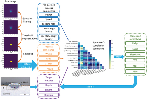
This research describes a semi-dynamic model incorporating machine learning techniques that gives insight into dynamic vertical melt pool dimensions (depth, height, dilution) by investigating the combined influence of process parameters (static) and limited in-situ monitoring data (dynamic). The workflow of this research is presented in Figure 1. Sixty single-track samples were prepared with different values of pre-defined process parameters, including laser power, scanning speed, and powder feed rate. The melt pool width, area, maximum temperature, and mean temperature indicators were extracted from the corresponding melt pool thermal videos. These were modelled as combined process parameters and used as input feature candidates for the semi-dynamic model. Based on Spearman<apos;>s rank correlation coefficient map, different input features were selected to predict melt pool depth, height, height, and dilution. The correlation between selected features and vertical melt pool dimensions was modelled via linear and nonlinear supervised ML techniques. Six different ML algorithms were implemented and compared based on their predictive capability for melt pool dimensions. The models presented in this paper demonstrate the potential to help achieve accurate melt pool dimension estimations in real-time with limited in-situ information.

Figure 1. Schematic description of the workflow applied in this study. The training set for the ML algorithms consists of three groups of data: pre-defined process parameters, process signatures extracted from in-situ image data, and target features. The input features were selected based on spearman<apos;>s correlation with target features. Six different ML algorithms were implemented and compared for predictive performance.

2. Methods and materials

2.1 Experimental setup

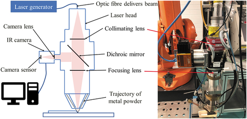
The LMD system consists of a 4 kW diode laser generator (LDF 4000–100, Laserline GmbH, Mülheim-Kärlich, Germany), a 0.6 mm optical transmission fibre that works in continuous wavelength mode within the range 980–1030 nm, a 6-axis robotic arm (IRB2400, ABB Ltd, Zürich, Switzerland), a powder feeder (Metco Twin 10-C, Sulzer Ltd, Winterthur, Switzerland), and a laser head; see Figure 2. The laser head was equipped with a collimating lens and a focusing lens to form a 2.5 mm diameter laser beam with a ‘top hat’ intensity distribution. The focal lengths of the lenses were 72 mm and 300 mm, respectively. A dichroic mirror was placed between the lenses at a 45° angle. The transmitting wavelength range of the mirror<apos;>s coating was in the range 800–1100 nm, within which the laser beam passes through the mirror, with radiation of wavelengths <800 nm and >1100 nm being reflected into the infrared (IR) camera. The coaxially mounted IR camera was an uncooled, middle wavelength infrared (MWIR) camera (TACHYON 16 K, New Infrared Technologies Ltd, Madrid, Spain) with a detector sensitive to spectral wavelengths between 1–5 µm and a peak detection wavelength of 3.7 µm. The detector chip featured a 128 ×128 array of pixels of dimensions 50 µm×50 µm. The IR camera<apos;>s lens had a focal length of 35 mm and an anti-reflective coating for spectral wavelengths between 1–5 µm. The pixels delivered a 16-bit monochrome signal at an image acquisition framerate of 50 Hz.

Figure 2. Schematic of the combined experimental apparatus, including laser head, infrared (IR) camera, and laser optics (fibre optic, collimating lens, dichroic mirror, and focusing lens).

2.2 Sample preparation

The metal powder was gas-atomised (spherical) SS316L powder (SS316L-5320, Höganäs AB, Höganäs, Sweden) with a particle size distribution between 45–125 µm. Sixty single-track samples were deposited using different process parameters (Table 1) at ambient laboratory conditions onto three mild steel strip substrates with dimensions 150 ×60 ×10 mm³. The process parameter ranges were selected empirically to avoid failed clads. The range of powder feed rates was initially selected as 5–11 RPM and then converted to 15.8–33.9 g/min. After deposition, each sample was sectioned at a position between 25–30 mm from the start of its track. The cross-sections were ground with 1200 grit SiC paper and etched using nital etchant (5% nitric acid). The track depth ($D$), height ($H$), and width ($W$) were measured using an Olympus DP27 microscope digital camera (Olympus Corporation, Shinjuku, Tokyo, Japan) at 10× magnification. Figure 3 presents a typical track cross-section (Trial 59). The melt pool dilution was calculated per Eq. 1(Eq. 1) $\mathrm{D}\mathrm{i}\mathrm{l}\mathrm{u}\mathrm{t}\mathrm{i}\mathrm{o}\mathrm{n}=\frac{D}{D+H}$(Eq. 1) (Cao et al. 2019).

(Eq. 1) $\mathrm{D}\mathrm{i}\mathrm{l}\mathrm{u}\mathrm{t}\mathrm{i}\mathrm{o}\mathrm{n}=\frac{D}{D+H}$(Eq. 1)

Figure 3. Cross-section of typical single-track deposition (Trial 59). $H$, $D$, and $W$ denote track height, depth, and width, respectively.

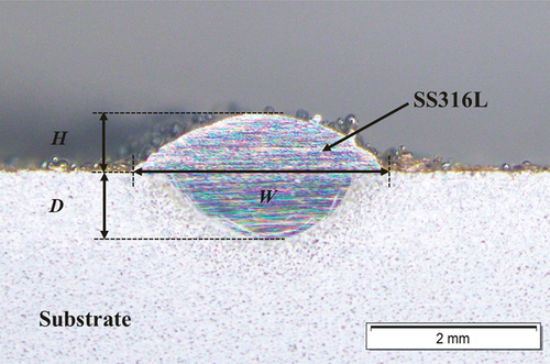
Table 1. Printing parameters used to fabricate all 60 single-track samples. The precisions of the laser power, scanning speed, and powder feed rate was 1 W, 1 mm/s, and 0.1 g/min, respectively

Trial no.	Laser power (kW)	Scanning speed (mm/s)	Powder feed rate (g/min)	Trial no.	Laser power (kW)	Scanning speed (mm/s)	Powder feed rate (g/min)
1	1	10	15.8	31	2.5	20	24.9
2	1	20	15.8	32	2.5	30	24.9
3	1	30	15.8	33	2.5	40	24.9
4	1	10	18.8	34	2.5	20	27.9
5	1	20	18.8	35	2.5	30	27.9
6	1	30	18.8	36	2.5	40	27.9
7	1	10	21.8	37	2.5	20	30.9
8	1	20	21.8	38	2.5	30	30.9
9	1	30	21.8	39	2.5	40	30.9
10	1.5	20	18.8	40	3	20	24.9
11	1.5	30	18.8	41	3	30	24.9
12	1.5	40	18.8	42	3	40	24.9
13	1.5	20	21.8	43	3	20	27.9
14	1.5	30	21.8	44	3	30	27.9
15	1.5	40	21.8	45	3	40	27.9
16	1.5	20	24.9	46	3	20	30.9
17	1.5	30	24.9	47	3	30	30.9
18	1.5	40	24.9	48	3	40	30.9
19	2	30	18.8	49	1.5	10	18.8
20	2	40	18.8	50	1.5	10	21.8
21	2	50	18.8	51	1.5	10	24.9
22	2	30	21.8	52	2.5	20	21.8
23	2	40	21.8	53	2.5	30	21.8
24	2	50	21.8	54	2.5	40	21.8
25	2	30	24.9	55	3	20	21.8
26	2	40	24.9	56	3	30	21.8
27	2	50	24.9	57	3	40	21.8
28	2	20	18.8	58	3	20	33.9
29	2	20	21.8	59	3	30	33.9
30	2	20	24.9	60	3	40	33.9

2.3 Image processing

Melt pool images were taken using a coaxially mounted IR camera and logged using the Tachyon 16 K Acquisition v5.15 software (New Infrared Technologies Ltd, Madrid, Spain. The framerate was 50 frames per second in this application. The keyframe at the cross-section of every single track was used for the melt pool dimension calculation. Among the selected frames, there were three typical patterns; see Table 2, column 1 for raw images. Two distinct regions are evident, namely a bright spot (melt pool) and a lighter sector that leads the melt pool and is highlighted with red ellipses in Table 2; these are due to the laser reflection from the inner surface of the nozzle. The melt pool region was smoothed by filtering the raw images using a 5 ×5 Gaussian kernel with a standard deviation $\sigma =1$; see Table 2, column 3. The solidus temperature of SS316L is ~1400°C (Tang, Tan, and Wong 2018), which was used as the threshold to extract the melted area, as shown in column 3. When the laser power was not relatively low (e.g. Trial 10), the melt pool could be accurately extracted from the image using an ellipse mask (Hofman et al. 2012). However, at relatively high laser power (e.g. Trial 55), the reflection from the nozzle remains after thresholding. Instead, the thresholded melt pool area for Trial 55 was located by setting an empirical melt pool size threshold. Any disconnected region below this value was rejected (Table 2, red rectangle). Note that the thresholded image for Trial 58 represents the most complex case found after threshold segmentation, i.e. for which a piece of the reflection area was both retained and combined with the melt pool region. For these cases, the melt pool area was extracted from the thresholded image by slicing the image row by row and calculating the row widths; see Figure 4. A third-order Savitzky-Golay filter was then applied to smooth the width distribution plot. The local minima were identified, and the local minima index was used to separate the reflection area from the melt pool area. Note that the above image processing and machine learning algorithms were implemented using PyCharm Professional 2021 (IntelliJ Software s.r.o., Prague, Czech Republic) equipped with a Python 3.7 interpreter. The major libraries applied in this study include NumPy, Pandas, Scikit-learn, and Matplotlib.

Figure 4. Row width distribution from the threshold segmentation image shown in Table 2, column 3, trial 58.

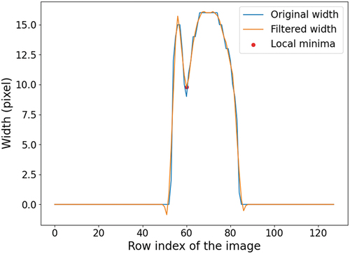
Table 2. Three typical raw melt pool images and their subsequent processing steps

Trial no.	Raw image	Gaussian filtering	Threshold segmentation	Ellipse fit
10
55
58

Figure 5 presents a comparison between the measured track width (Olympus DP27 microscope, Olympus Corporation, Shinjuku, Tokyo, Japan) and the melt pool width after the additional image processing steps described above. Four error evaluations were obtained from Figure 5 and are presented in Table 3, namely the Mean Absolute Error (MAE), Maximum Absolute Error (MXAE), Mean Absolute Percent Error (MAPE), and Maximum Absolute Percent Error (MXAPE); see Eq. 2(Eq. 2) $\mathrm{M}\mathrm{A}\mathrm{E}=\frac{1}{n}\sum _{i=1}^n\left|y_i-{\hat{y}}_i\right|$(Eq. 2) –5(Eq. 5) $\mathrm{M}\mathrm{X}\mathrm{A}\mathrm{P}\mathrm{E}=max\left\{x:x\in \mathrm{M}\mathrm{A}\mathrm{P}\mathrm{E}\right\}$(Eq. 5) , where $y$ is the true value of the dataset and $\hat{y}$ is the prediction. The MAPE was 1.8%, and the MXAPE was less than 10%, indicating the extracted melt pool width was relatively close to the measured track width, thus demonstrating the reliability of the image processing algorithms. Finally, the associated melt pool area and temperature (mean and maximum) were estimated using the data for the extracted melt pool regions.

(Eq. 2) $\mathrm{M}\mathrm{A}\mathrm{E}=\frac{1}{n}\sum _{i=1}^n\left|y_i-{\hat{y}}_i\right|$(Eq. 2)

(Eq. 3) $\mathrm{M}\mathrm{X}\mathrm{A}\mathrm{E}=max\left\{x:x\in \mathrm{M}\mathrm{A}\mathrm{E}\right\}$(Eq. 3)

(Eq. 4) $\mathrm{M}\mathrm{A}\mathrm{P}\mathrm{E}=\frac{1}{n}\sum _{i=1}^n\frac{\left|y_i-{\hat{y}}_i\right|}{y_i}$(Eq. 4)

(Eq. 5) $\mathrm{M}\mathrm{X}\mathrm{A}\mathrm{P}\mathrm{E}=max\left\{x:x\in \mathrm{M}\mathrm{A}\mathrm{P}\mathrm{E}\right\}$(Eq. 5)

Figure 5. (a) Comparison between the track width measured via an optical microscope and the melt pool width after all the image processing steps described in section 2.3. The (b) absolute errors between two widths.

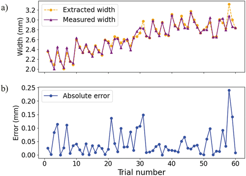
Table 3. Error evaluations between track width measured via an optical microscope and the melt pool width after all the image processing steps described in section 2.3. The precisions of MAE and MXAE are $\pm$ 1 µm

MAE (mm)	MXAE (mm)	MAPE (%)	MXAPE (%)
0.043	0.240	1.8	8.3

2.4 Feature selection

The dataset for feature selection consists of the predefined process parameters, i.e. laser power ($LP$), scanning speed ($SS$), powder feed rate ($FR$), line energy density ($LED$), specific energy density ($SED$), measured track geometries, i.e. depth ($D$), height ($H$), and dilution ($Di$), along with the extracted melt pool features, i.e. melt pool width ($W$), area ($A$), mean ($T_{mean}$), and max temperature ($T_{max}$) indicators. $LED$ and $SED$ are defined by Eq. 6(Eq. 6) $LED=\frac{LP}{SS}\left(\frac{\mathrm{J}}{\mathrm{m}\mathrm{m}}\right)$(Eq. 6) (DebRoy et al. 2018) and Eq. 7(Eq. 7) $SED=\frac{LP}{FR}\left(\frac{\mathrm{J}}{\mathrm{g}}\right)$(Eq. 7) (Li et al. 2019), respectively. Melt pool area ($A$) is defined as the projection of melt pool surface area on the horizontal plane. $T_{mean}$ and $T_{max}$ were calculated from the individual pixel intensities within the melt pool area. $D$, $H$, and $Di$ were the targets, and all remaining features were input candidates ($LP$, $SS$, $FR$, $LED$, $SED$, $W$, $A$, $T_{max}$, $T_{mean}$).

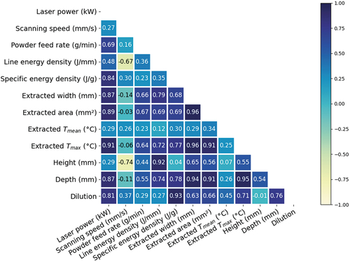
To avoid blindly using all input features to correlate with the target variables, significant input features on each target were selected using Spearman<apos;>s rank correlation coefficient matrix; this was chosen as it focuses on the monotonic trend between paired data but not their values (Figure 6). Spearman<apos;>s coefficient $\rho$ is defined by Eq. 8(Eq. 8) $\rho =\frac{\mathrm{c}\mathrm{o}\mathrm{v}\left(r_x,r_y\right)}{{\sigma }_{rx}{\sigma }_{ry}}$(Eq. 8) (Spearman 1961), in which $\mathrm{c}\mathrm{o}\mathrm{v}()$ is the covariance,$r_x,r_y$ are the ranked paired features, and ${\sigma }_{rx},{\sigma }_{ry}$ are the standard deviations of $r_x$ and $r_y$, respectively. Coefficient values close to −1 and 1 mean a strong negative and positive monotonic relationship, respectively, between the paired features. In this study, $\rho >0.6$ is considered a strong correlation (Myers, Well, and Frederick Lorch 2010). Following the above process, $SS$, $LED$, and $W$ are the significant input features for correlating with $H$. Similar selection processes were implemented for correlating melt pool depth and dilution.

(Eq. 6) $LED=\frac{LP}{SS}\left(\frac{\mathrm{J}}{\mathrm{m}\mathrm{m}}\right)$(Eq. 6)

(Eq. 7) $SED=\frac{LP}{FR}\left(\frac{\mathrm{J}}{\mathrm{g}}\right)$(Eq. 7)

(Eq. 8) $\rho =\frac{\mathrm{c}\mathrm{o}\mathrm{v}\left(r_x,r_y\right)}{{\sigma }_{rx}{\sigma }_{ry}}$(Eq. 8)

Figure 6. Spearman<apos;>s rank correlation coefficient map for each variable pairing from the predefined process parameters extracted melt pool features and measured track geometries.

2.5 Machine learning models design

Six different supervised ML techniques were designed and evaluated for this research, including three linear regression models (Lasso, Ridge, ElasticNet) and three nonlinear models (support vector regression, ‘SVM’; K-neighbours regression, ‘KNR’; artificial neural network, ‘ANN’). The input/output variables for each are presented in Table 4. The performance of machine learning algorithms is highly affected by hyperparameters, with inappropriate choices resulting in either underfitting or overfitting the input data. This aspect of the design decision is detailed below.

Table 4. Input and output variables for all machine learning models tested here

Lasso, Ridge, ElasticNet, SVR, KNR		ANN characteristics
Inputs	Output	Inputs	Outputs
$LP$, $LED$, $SED$, $W$, $A$, $T_{max}$	$D$	$LP$, $SS$, $LED$, $SED$, $W$, $A$, $T_{max}$	$D$, $H$, $Di$
$SS$, $LED$, $W$	$H$	$LP$, $SS$, $FR$, $LED$, $SED$, $W$, $A$, $T_{max}$, $T_{mean}$	$D$, $H$, $Di$
$LP$, $SED$, $W$, $A$, $T_{max}$	$Di$

2.5.1 Lasso, ridge, and elasticnet

Lasso, Ridge, and ElasticNet are multi-input, single-output linear regression algorithms. The reason for selecting these linear regression algorithms is that they were developed for data fitting with multi-variate problems, as this was the case here. They were also applied successfully to cost estimation for a fused filament fabrication system and demonstrated promising predictive capability (Chan, Yanglong, and Wang 2018). These linear regression algorithms differ in the regularisation method employed by the cost function, which optimises the weights of the linear regression function. The main tunable hyperparameter is then the regularisation parameter $\lambda$; see Table 5. Large values specify stronger regularisation (avoids overfitting), although excessively large values promote underfitting. For ElasticNet, the additional ‘ratio parameter’ $\alpha$ (0–1) controls the strength of the L1 norm regularisation (Table 5).

Table 5. Hyperparameter candidates for different supervised machine learning algorithms used in this research

Algorithms	Hyperparameter	Description	Candidates
Ridge	$\lambda$	L2 regularisation parameter	10^–3, 10^–2, 10^–1, 1, 10
Lasso	$\lambda$	L1 regularisation parameter	10^–3, 10^–2, 10^–1, 1, 10
ElasticNet	$\lambda$	L2 regularisation parameter	10^–3, 10^–2, 10^–1, 1, 10
	$\alpha$	The ratio of L2 `	0.25, 0.5, 0.75
SVR	$K\left(x\right)$	Kernel functions	polynomial, RBF, sigmoid
	$C=\frac{1}{2\lambda }$	L2 regularisation parameter	10^–3, 10^–2, 10^–1, 1, 10
	$d$	Degree of the polynomial kernel	2, 3
KNR	$k$	Number of neighbours	3, 4, 5, 6, 7
ANN	$\lambda$	L2 regularisation parameter	10^–3, 10^–2, 10^–1, 1
	$n_{neuron}$	Neuron number	1, 2, …, 2 n +3 (n = inputs)
	$n_{layer}$	Hidden layer number	1, 2
	$\phi \left(x\right)$	Activation function	Relu, Logistic
		Learning rate mode	Adaptive, Constant

A grid search algorithm was implemented to select optimal hyperparameter candidates. All inputs and outputs were scaled to [−1, 1] to improve performance. The scaled dataset was then split into a training set (80%) and a testing set (20%) (Géron 2019). Threefold cross-validation (CV) was implemented in the training set for the hyperparameter candidates. Optimal hyperparameters were then selected based on the average mean squared error (MSE) from the threefold CV step; see Table 6.

Table 6. Optimised hyperparameter for all machine learning models tested here

Models	Depth	Height	Dilution
Lasso	$\lambda$=10^−3	$\lambda$=10^−2	$\lambda$=10^−3
Ridge	$\lambda$=10^−3	$\lambda$=10^−1	$\lambda$ =10^−3
ElasticNet	$\lambda$=10^−3, $\alpha$ =0.25	$\lambda$=10^−2,$\alpha$=0.5	$\lambda$=10^−3, $\alpha$ =0.25
SVR	$C$=1, RBF kernel	$C$=10, RBF kernel	$C$=10, RBF kernel
KNR	$k$=6	$k$=7	$k$=4
ANN [7 11 3]	Relu, $\lambda$=10^−3, constant learning rate: 0.01
ANN [7 17 8 3]	Relu, $\lambda$=10^−3, constant learning rate: 0.01
ANN [9 14 3]	Relu, $\lambda$=10^−2, constant learning rate: 0.01
ANN [9 17 9 3]	Relu, $\lambda$=10^−2, constant learning rate: 0.01

2.5.2 SVR and KNR

SVR and KNR are multi-input, single-output nonlinear regression algorithms. Their prediction functions were used in high-dimensional pattern recognition and solving nonlinear problems. They have been applied for as-built chemical composition estimation (Song et al. 2017) and mechanical properties estimation (Xie et al. 2021) in the application of LMD. SVR generalises support vector machine (SVM) that returns continuously valued outputs (Awad and Khanna 2015). Its core concept is to determine a $\epsilon$-tube with maximal data points in the $\epsilon$-distance margin by balancing model complexity against prediction error. The $\epsilon$ value chosen here is 0.1. For nonlinear cases, to find an optimised $\epsilon$-tube, the feature data must be mapped into a higher dimensional space. This is achieved via the kernel functions (Table 5).

The KNR estimator<apos;>s outputs are calculated as the interpolated value between each testing point<apos;>s nearest neighbours as chosen from the training dataset (Matthew et al. 2021); in this case, ‘nearest’ refers to the Euclidean distance. Using a larger-valued neighbour number $k$ permits more accurate interpolation but introduces higher computational cost. Thus, $k$ controls the performance of the prediction method; see Table 5. Similarly, the optimised hyperparameters for SVR and KNR were selected based on the average mean squared error (MSE) of the threefold CV step; see Table 6.

2.5.3 ANN

The ANN method is a powerful technique for constructing the complex, nonlinear relationship (‘mapping’) between a system<apos;>s inputs and outputs. The ANN model is based on a training dataset, while its performance depends on a series of parameters, including the choice of model inputs and the chosen relationship, i.e. network structure (Daiki et al. 2019). It has been confirmed in the literature that ANN models provide accurate predictions of process parameters (Caiazzo and Caggiano 2018) and cross-sectional track geometry (Feenstra, Molotnikov, and Birbilis 2021), which will contribute to a successful rate in this study. Two input vectors were implemented here, namely (i) all the input features except $FR$ and $T_{mean}$, as both their Spearman<apos;>s coefficient with $D$, $H$, and $Di$ were <0.6, and (ii) all nine input features.

Due to ANN<apos;>s flexible model (or structure), MSE cannot straightforwardly evaluate the relative performance of ANN structures with different input features. Therefore, four different ANN structures and their corresponding optimised hyperparameters are presented in Table 5. The maximum hidden layer number, $n_{layer}$, was set at two to avoid overfitting. For the single-hidden-layer ANNs, ANN [7 11 3] and ANN [9 14 3], the neuron number, $n_{neuron}$, in the hidden layer was varied from unity to 2 n +3 where ‘n’ is the number of input features. Note that the numbers in the square bracket after ‘ANN’ represent the structure of the ANN. The first number represents the inputs, and the last indicates the outputs. The number between the input and output represents the neuron number for each hidden layer. The optimised $n_{neuron}$ was selected based on the average MSE of the threefold CV. For $n_{layer}=2$ (ANN [7 17 8 3] and ANN [9 17 9 3]), the neuron number in the first layer ($n_{neuron}^{\left(1\right)}$) was similarly varied from unity to 2 n +3. The neuron number in the second layer ($n_{neuron}^{\left(2\right)}$) was also traversed from unity to 2 n +3, but it was always $\le n_{neuron}^{\left(1\right)}$.

3. Results and discussion

This section presents results for all nine ML models tested here. These models predict melt pool depth, height, and dilution, with predictivity rated using the Mean Absolute Error (MAE), Maximum Absolute Error (MXAE), Mean Absolute Percent Error (MAPE), and Maximum Absolute Percent Error (MXAPE) measures. The relative accuracy of these models when predicting melt pool depth, height, and dilution are presented in Sections 3.1, 3.2, and 3.3, respectively.

3.1 Evaluation of machine learning models for depth prediction

Table 7 shows the R² values obtained from each machine learning model when predicting the depth of the melt pool. This parameter is widely used in regression analysis for characterising the proportion of variation in a response quantity explained by a linear correlation model with an input quantity. For depth prediction, the training score for the Lasso model is 0.948, which shows that the model fits the training data well. The CV score is slightly less than the training score, indicating that the trained Lasso model is not overfitted and can be generalised to independent new data. The testing score for the Lasso model also indicates good performance as the testing and training scores are very similar (<0.05 difference).

Table 7. R² values for all machine learning models tested here. These data characterise how well each regression model fits the observed data (measured melt pool depth, height, and dilution) for each train, CV, and test datasets

Models	Depth			Height			Dilution
	Train	CV	Test	Train	CV	Test	Train	CV	Test
Lasso	0.948	0.921	0.913	0.882	0.809	0.787	0.931	0.910	0.883
Ridge	0.950	0.927	0.910	0.885	0.804	0.761	0.933	0.915	0.882
ElasticNet	0.949	0.925	0.912	0.883	0.809	0.779	0.932	0.913	0.883
SVR	0.973	0.934	0.958	0.940	0.784	0.846	0.976	0.935	0.956
KNR	0.921	0.908	0.937	0.845	0.752	0.734	0.930	0.911	0.904
ANN [7 11 3]	0.983	0.887	0.948	0.972	0.955	0.961	0.968	0.947	0.933
ANN [7 17 8 3]	0.987	0.908	0.953	0.960	0.916	0.947	0.982	0.934	0.938
ANN [9 14 3]	0.990	0.909	0.957	0.978	0.970	0.969	0.976	0.928	0.925
ANN [9 17 9 3]	0.988	0.910	0.958	0.981	0.963	0.948	0.983	0.937	0.947

The three linear models (Lasso, Ridge, ElasticNet) all have R² values within 0.01 for the training, CV, and testing scores, respectively, which indicates they have very similar performance when predicting melt pool depth. KNR gives slightly lower training and CV scores than the linear models, but its testing score is higher than the linear models by a larger margin (>0.02). The highest testing scores overall were achieved jointly by SVR and ANN [9 17 9 3], with SVR also achieving the highest CV score. Finally, all four ANN model structures train and test R² scores were within 0.01.

Whilst the R² measure is straightforwardly calculated, its rigour is limited when used with small datasets (Colton and Bower 2002). In this study, the number of samples is 60, and the number of testing samples is limited to 12, arguably approaching ‘small’. Therefore, further correlation measures were tested here, including the MAE, MXAE, MAPE, and MXAPE, as listed in Table 8.

Table 8. Error measure values when predicting melt pool depth for all machine learning models tested here. The rank assigned to each model is calculated from its mean rank when the models are compared according to their MAE, MXAE, MAPE, and MXAPE values. The precisions of the dimensioned error measures, MAE and MXAE, are both $\pm$ 1 µm

Models	MAE (mm)	MXAE (mm)	MAPE (%)	MXAPE (%)	Rank
Lasso	0.070	0.141	57	343	9
Ridge	0.070	0.140	55	341	7
ElasticNet	0.070	0.140	56	341	7
SVR	0.044	0.132	30	159	4
KNR	0.054	0.119	32	124	3
ANN [7 11 3]	0.049	0.139	34	157	6
ANN [7 17 8 3]	0.039	0.153	18	78	4
ANN [9 14 3]	0.041	0.144	17	44	2
ANN [9 17 9 3]	0.036	0.127	11	30	1

The MAEs and their standard deviations when predicting melt pool depth are plotted in Figure 7 for the training and testing datasets. At the same time, the raw values are presented in Table 12 in the Supplementary Information. The linear models and ANN [9 17 9 3] give the highest and lowest MAE for the testing results, respectively. Interestingly, while SVR gives the highest testing R² score, its corresponding MAE is not the lowest.

Table 8 demonstrates that the linear models (Lasso, Ridge, ElasticNet) give the highest MAEs, which is near twice the lowest MAE as achieved by ANN [9 17 9 3]. The MXAEs of the linear model is not the highest, but they contribute to the highest MXAPE (>300%), which is unacceptably high. The MAPEs of the linear models are also quite high, which indicates that each melt pool depth prediction will have >50% error on average. Thus, the input features are not linearly correlated with melt pool depth. The highest MXAE is obtained by ANN [7 17 8 3], but it does not cause the highest MXAPE. Even though KNN has the smallest MXAE, it still contributes to an unacceptably high MXAPE (>100%). The MAPEs for SVR and ANN [7 11 3] are ~20% smaller than the linear models, but their MXAPEs are >100%, i.e. unacceptably high. The lowest MAE, MAPE, and MXAPE with respect to depth prediction are achieved by ANN [9 17 9 3] at 0.036 mm, 11%, and 30%, respectively.

The above error measures were combined into a collective rank for each model with respect to melt pool depth prediction (Table 8). These are based on the mean of their integer ranks obtained for each error measure. For example, the MAE of ANN [9 17 9 3] in Table 8 is the smallest, and thus its MAE-specific rank was assigned at unity, while its rank for MXAE was the second smallest, and thus, its MXAE-specific rank was assigned at two. The rank value increases with decreasing model performance for all error measures when predicting melt pool depth.

Figure 7. Mean Absolute Error (MAE) and standard deviation for melt pool depth prediction for all machine learning models tested here.

3.2 Evaluation of machine learning models for height prediction

A similar phenomenon as described in section 3.1 for melt pool depth prediction was observed for the linear models and melt pool height prediction, i.e. they demonstrate R² values within 0.01 for the training, CV, and testing scores; see Table 7. However, the linear models did not fit the height or depth prediction data as their training scores were < 0.9. The CV and testing scores were lower than the corresponding training scores, implying that linear correlation is inappropriate for predicting melt pool height from the input features chosen here.

Regarding the nonlinear models tested here, the training score for SVR was > 0.9, but the CV and testing scores were both $\ge$ 10% lower than the training score. The large gap between the training and CV scores (~15%) implies the model developed here was overfitted even after optimising the hyperparameters using threefold CV. The KNR model scores were even lower than the linear models, implying that the KNR model is inappropriate for predicting melt pool height. The ANN models tested here featured high training, CV, and testing scores for melt pool height prediction.

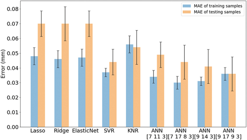
The MAEs and their standard deviations for melt pool height prediction are presented in Figure 8 for the training and testing results; see Supplementary Information (Table 13) for raw values. The models tested here fall into two performance groups based on MAE, namely ANN and non-ANN models. The ANN models demonstrate significant lower MAEs for both training and testing results. Table 9 presents the error evaluations for the testing results for all models. The MAEs and MXAEs for the non-ANN models were similar at ~0.06 mm and ~0.11 mm, respectively. These models also yield similar MAPEs (~16%) and MXAPEs (~30%), except for KNR (MXAPE = 52%). Even though the R² values of non-ANN models for height prediction were not as high as for melt pool depth prediction, the MAPEs and the MXAPEs were significantly smaller. Finally, for all ANN models, the MAE and MXAE for height prediction were ~0.25 mm and ~0.5 mm, respectively, and the corresponding MAPE and MXAPE were ~7% and ~20%, respectively. The best performance was achieved by ANN [9 14 3].

Figure 8. Mean Absolute Error (MAE) and standard deviation for melt pool height prediction for all machine learning models tested here.

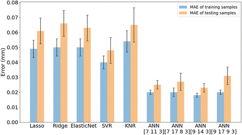
Table 9. Error measure values when predicting melt pool height for all machine learning models tested here. The rank assigned to each model was calculated from its mean rank when the models were compared by their MAE, MXAE, MAPE, and MXAPE values. The precisions of the dimensioned error measures, MAE and MXAE, are $\pm$ 1 µm

Models	MAE (mm)	MXAE (mm)	MAPE (%)	MXAPE (%)	Rank
Lasso	0.061	0.113	16	26	5
Ridge	0.066	0.118	18	27	8
ElasticNet	0.063	0.115	16	27	7
SVR	0.048	0.114	13	30	6
KNR	0.065	0.139	18	52	9
ANN [7 11 3]	0.026	0.054	8	21	2
ANN [7 17 8 3]	0.024	0.077	7	26	3
ANN [9 14 3]	0.023	0.040	7	17	1
ANN [9 17 9 3]	0.030	0.056	8	16	3

3.3 Evaluation of machine learning models for dilution prediction

The training score of the Lasso model for dilution prediction is 0.931, i.e. well-fitted, which then achieves still high (but slightly decreased) CV and testing scores. The three linear models (Lasso, Ridge, ElasticNet) achieve R² values within 0.01 for their training, CV, and testing scores indicating highly similar predictive performance for melt pool dilution. Based on the R² values of training, CV, and testing sets from Table 7, these models lie in two groups: linear models plus KNR (slightly lower R²) and SVR plus ANN (higher R²). The SVR model achieved the highest testing R² score.

Figure 9 presents the MAEs and their standard deviations for the training and testing datasets for melt pool dilution prediction; see Supplementary Information, Table 14 for raw data. The SVR model has the lowest MAEs for both training and testing results. The MAE results show that the model with higher R² values has lower MAEs. More generally, the detailed error evaluations of predictive performance for developed models are presented in Table 10. The MAEs for the testing datasets were similar to all models except SVR (lowest MAE). The MXAE and MAPE show a similar trend as the MAE, with SVR achieving the minimum MXAE and MAPE. The MXAE and MAPE of ANN [9 17 9 3] were very similar to the SVR model. The MXAPEs of the linear models were >150% (unacceptably high). Overall, the SVR model achieved the best performance for dilution prediction, with the linear models all significantly worse.

Figure 9. Mean Absolute Error (MAE) and standard deviation for melt pool dilution prediction for all machine learning models tested here.

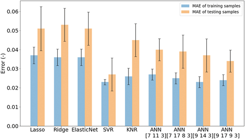
Table 10. Error measure values when predicting melt pool dilution for all machine learning models tested here. The rank assigned to each model is calculated from its mean rank when the models are compared by their MAE, MXAE, MAPE, and MXAPE values

Models	MAE (-)	MXAE (-)	MAPE (%)	MXAPE (%)	Rank
Lasso	0.051	0.104	25	175	7
Ridge	0.053	0.111	24	162	9
ElasticNet	0.051	0.107	25	171	7
SVR	0.027	0.072	8	25	1
KNR	0.045	0.120	20	75	6
ANN [7 11 3]	0.040	0.092	15	58	5
ANN [7 17 8 3]	0.038	0.087	12	41	3
ANN [9 14 3]	0.037	0.105	13	40	4
ANN [9 17 9 3]	0.034	0.078	10	26	2

3.4 Relative predictive performance of machine learning models

Table 7 values indicate how well the predicted dataset from an ML model matches the target dataset. However, it cannot demonstrate how well the predicted dataset matches the target dataset quantitatively. For example, SVR and ANN [9 17 9 3] have the same R² score for the melt pool depth testing dataset, but SVR has larger MAE and MXAE. By the same logic, the quantitative predictive accuracies of the ML algorithms for the target datasets also cannot be compared using R² scores, e.g. the linear models have testing scores ~0.91 and ~0.77 for melt pool depth and height prediction, respectively. However, the MAPEs for the linear models for depth prediction (~55%) was more than triple that for height prediction (~16%). Therefore, errors between the predicted and experimental testing datasets must be investigated in more detail.

The algorithms implemented in this study include both single-output and multi-output models. The best-performing model cannot be selected by evaluating its predictive performance for a single target. Therefore, a rank-based evaluation was used, as listed in Table 11. The models’ ranks for depth, height, and dilution predictive performance were adopted from Tables 8–10, and their average values were calculated. Generalised predictive performance, therefore, increases as average rank decreases. By these metrics, ANN [9 17 9 3] was the best-performing model at correlating the nine input features with the three output target datasets studied here.

Table 11. Rank values for predicting melt pool depth, height, and dilution for all the machine learning models tested in this investigation. A smaller average rank indicates the better overall performance of the model

Models	Rank
	Depth	Height	Dilution	Average
Lasso	9	5	7	7.0
Ridge	7	8	9	8.0
ElasticNet	7	7	7	7.0
SVR	4	6	1	3.7
KNR	3	9	6	6.0
ANN [7 11 3]	6	2	5	4.3
ANN [7 17 8 3]	4	3	3	3.3
ANN [9 14 3]	2	1	4	2.3
ANN [9 17 9 3]	1	3	2	2.0

Two more sectionings were taken at positions 10 mm and 40 mm from the start of the tracks to validate the predictions from the chosen model ANN [9 17 9 3]. The dimensions of the cross-sections are presented in Figure 10 (orange diamonds). The dimensions of the samples varied during the printing process; note that while these differences during short single-track depositions are not significant, they are very likely to change more significantly during 3D component fabrication due to heat accumulation and steeper local thermal gradients causing instability of the melt pool<apos;>s dimensions. However, the semi-dynamic model presented here can estimate melt pool dimensions in real-time. The predictions of each melt pool dimension throughout the printing process were calculated using the trained ANN [9 17 9 3] model with combined input data as shown in Figure 10 (blue dots). This model provides good predictions, requiring the combined static parameters and dynamic sensing data as inputs.

Figure 10. Comparison between the predictions from ANN [9 17 9 3] and measurements from the cross-sections of a single-track build (Trial 40).

4. Conclusions

This study demonstrates the potential for establishing a semi-dynamic machine learning model for online melt pool feature prediction. The models tested here were calibrated to geometric measurements and melt pool thermal images from sixty single-track depositions fabricated using different combinations of critical process parameters, including laser power, scanning speed, and powder feed rate. The input features of the model combined the process parameters (static) and features extracted from the in-situ melt pool images (dynamic). Significant input features to output targets were selected based on Spearman<apos;>s rank correlation coefficient. The output targets were the melt pool depth, height, and dilution, which have major effects on the track geometry, and by extension, the finished component geometry and quality. The connection between the selected input features and output targets was trained using linear regression models (Lasso, Ridge, ElasticNet), non-linear regression models (SVR, KNR), and artificial neural network models (ANN). Key results and conclusions are as follows:

• The melt pool features (depth, height, and dilution) are well predicted when using the combination of the process parameters and melt pool image features selected here

• Regarding depth prediction, the MAPEs and MXAPEs of linear regression models were >50% and >300%, respectively, which indicated the correlation between depth and hybrid inputs was highly nonlinear. SVR and KNR had fewer MAPEs (~30%) and MXAPEs (>100%), but their estimations were still not acceptable. The best depth estimation performance was obtained by ANN [9 17 9 3], whose MAPE and MXAPE were 11% and 30%, respectively.

• Concerning height prediction, the MAPEs and MXAPEs of all the models were <20% and <30%, respectively, except the MXAPE of the KNR model (52%). Linear regression models had similar MAPEs and MXAPEs with SVR ~15% and ~30, respectively. The lowest MAPE (7%) was achieved by ANN [9 14 3] and ANN [7 17 8 3], and the lowest MXAPE was achieved by ANN [9 17 9 3].

• For dilution prediction, linear regression models had the highest MAPEs and MXAPEs at>20% and >150%, respectively. The MAPEs of KNR and all ANNs were in the range of 10–20%. SVR and ANN [9 17 9 3] have very close MAPEs, and the SVR model achieved MXAPEs and the best performance.

• Six different machine learning algorithms were implemented. Based on overall performance at melt pool depth, height, and dilution prediction, ANN [9 17 9 3] achieved the best performance from the machine learning models tested here.

This study predicted the melt pool dimensions based on the hybrid process parameters and sensing data. However, it is not enough to improve the 3D part geometry accuracy since more parameters have not been considered in ML models, such as the z-increment, hatch spacing, and tool path planning, which significantly impact final part geometry. Therefore, future work will analyse the effects of the parameters above on 3D part geometry and rebuild the data-driven structure to estimate the geometry and defects in real-time for the 3D part fabrication.

Acknowledgments

The authors acknowledge the financial support provided by the Commonwealth Scientific and Industrial Research Organisation (CSIRO) and its Active Integrated Matter Future Science Platform (AIM FSP) [Testbed number: AIM FSP_TB10_WP05]. The authors also would like to acknowledge Hans Lohr and Con Filippou for their support on configuring the experimental setup.

Disclosure statement

No potential conflict of interest was reported by the author(s).

Additional information

Funding

This work was supported by the Commonwealth Scientific and Industrial Research Organisation (CSIRO) [AIM FSP_TB10_WP05].

References

- Ansari, M., R. Shoja Razavi, and M. Barekat. 2016. “An Empirical-statistical Model for Coaxial Laser Cladding of NiCrAlY Powder on Inconel 738 Superalloy.” Optics & Laser Technology 86: 136–144. doi:10.1016/j.optlastec.2016.06.014.
- Awad, M., and R. Khanna. 2015. “Support Vector Regression,” In Efficient Learning Machines: Theories, Concepts, and Applications for Engineers and System Designers, edited by Pepper, J., Weiss, S., Hauke, P., 67–80, Berkeley, CA: Apress. doi:10.1007/978-1-4302-5990-9_4.
- Bax, B., R. Rajput, R. Kellet, and M. Reisacher. 2018. “Systematic Evaluation of Process Parameter Maps for Laser Cladding and Directed Energy Deposition.” Additive Manufacturing 21: 487–494. doi:10.1016/j.addma.2018.04.002.
- Brian, G., Y. Kumar Bandari, B. Richardson, A. Roschli, B. Post, M. Borish, A. S. Thornton, W. C. Henry, M. D. Lamsey, and L. Love. 2019. “Melt pool monitoring for control and data analytics in large-scale metal additive manufacturing.“ 2019 International Solid Freeform Fabrication Symposium, August 12-14, 2019, Austin, Texas, USA.
- Caiazzo, F., and A. Caggiano. 2018. “Laser Direct Metal Deposition of 2024 Al Alloy: Trace Geometry Prediction via Machine Learning.” Materials (Basel) 11 (3): 444. doi:10.3390/ma11030444.
- Cao, L., S. Chen, M. Wei, Q. Guo, J. Liang, C. Liu, and M. Wang. 2019. “Effect of Laser Energy Density on Defects Behavior of Direct Laser Depositing 24CrNiMo Alloy Steel.” Optics & Laser Technology 111: 541–553. doi:10.1016/j.optlastec.2018.10.025.
- Chan, S. L., L. Yanglong, and Y. Wang. 2018. “Data-driven Cost Estimation for Additive Manufacturing in Cybermanufacturing.” Journal of Manufacturing Systems 46: 115–126. doi:10.1016/j.jmsy.2017.12.001.
- Colton, J. A., and K. M. Bower. 2002. “Some Misconceptions about R2.” accessed October 2021.
- Daiki, I., A. Vargas-Uscategui, W. Xiaofeng, and P. C. King. 2019. “Neural Network Modelling of Track Profile in Cold Spray Additive Manufacturing.” Materials (Basel, Switzerland) 12 (17). doi:10.3390/ma12172827.
- DebRoy, T., H. L. Wei, J. S. Zuback, T. Mukherjee, J. W. Elmer, J. O. Milewski, A. M. Beese, A. Wilson-Heid, A. De, and W. Zhang. 2018. “Additive Manufacturing of Metallic Components – Process, Structure and Properties.” Progress in Materials Science 92: 112–224. doi:10.1016/j.pmatsci.2017.10.001.
- Ding, Y., J. Warton, and R. Kovacevic. 2016. “Development of Sensing and Control System for Robotized Laser-based Direct Metal Addition System.” Additive Manufacturing 10: 24–35. doi:10.1016/j.addma.2016.01.002.
- Errico, V., S. L. Campanelli, A. Angelastro, M. Dassisti, M. Mazzarisi, and C. Bonserio. 2021. “Coaxial Monitoring of AISI 316L Thin Walls Fabricated by Direct Metal Laser Deposition.” Materials (Basel) 14 (3): 673. doi:10.3390/ma14030673.
- Feenstra, D. R., A. Molotnikov, and N. Birbilis. 2021. “Utilisation of Artificial Neural Networks to Rationalise Processing Windows in Directed Energy Deposition Applications.” Materials & Design 198: 109342. doi:10.1016/j.matdes.2020.109342.
- Géron, A. 2019. Hands-on Machine Learning with Scikit-Learn, Keras, and TensorFlow: Concepts, Tools, and Techniques to Build Intelligent Systems. Sebastopol, California, United States: O’Reilly Media, Inc.
- Guijun, B., A. Gasser, K. Wissenbach, A. Drenker, and R. Poprawe. 2006. “Identification and Qualification of Temperature Signal for Monitoring and Control in Laser Cladding.” Optics and Lasers in Engineering 44 (12): 1348–1359. doi:10.1016/j.optlaseng.2006.01.009.
- Gunasegaram, D. R., A. B. Murphy, A. Barnard, T. DebRoy, M. J. Matthews, L. Ladani, and D. Gu. 2021. “Towards Developing Multiscale-multiphysics Models and Their Surrogates for Digital Twins of Metal Additive Manufacturing.” Additive Manufacturing 46 (102089): 102089. doi:10.1016/j.addma.2021.102089.
- Hofman, J. T., B. Pathiraj, J. van Dijk, D. F. de Lange, and J. Meijer. 2012. “A Camera Based Feedback Control Strategy for the Laser Cladding Process.” Journal of Materials Processing Technology 212 (11): 2455–2462. doi:10.1016/j.jmatprotec.2012.06.027.
- Jiang, J., and F. Yun-Fei. 2020. “A Short Survey of Sustainable Material Extrusion Additive Manufacturing.” Australian Journal of Mechanical Engineering 1–10. doi:10.1080/14484846.2020.1825045.
- Jingchao, J., S. T. Newman, and R. Y. Zhong. 2020. “A Review of Multiple Degrees of Freedom for Additive Manufacturing Machines.” International Journal of Computer Integrated Manufacturing 34 (2): 195–211. doi:10.1080/0951192x.2020.1858510.
- Jingchao, J., Y. Xiong, Z. Zhang, and D. W. Rosen. 2020. “Machine Learning Integrated Design for Additive Manufacturing.” Journal of Intelligent Manufacturing. doi:10.1007/s10845-020-01715-6.
- Li, J., H. Ren, C. Liu, and S. Shang. 2019. “The Effect of Specific Energy Density on Microstructure and Corrosion Resistance of CoCrMo Alloy Fabricated by Laser Metal Deposition.” Materials (Basel) 12 (8). doi:10.3390/ma12081321.
- Matthew, D., M. A. Wonders, M. Flaska, and A. T. Lintereur. 2021. “K-Nearest Neighbors Regression for the Discrimination of Gamma Rays and Neutrons in Organic Scintillators.” Nuclear Instruments Methods in Physics Research Section A: Accelerators, Spectrometers, Detectors Associated Equipment 987: 164826. doi:10.1016/j.nima.2020.164826.
- Meng, L., B. McWilliams, W. Jarosinski, H.-Y. Park, Y.-G. Jung, J. Lee, and J. Zhang. 2020. “Machine Learning in Additive Manufacturing: A Review.” Jom 72 (6): 2363–2377. doi:10.1007/s11837-020-04155-y.
- Mukherjee, T., and T. DebRoy. 2019. “A Digital Twin for Rapid Qualification of 3D Printed Metallic Components.” Applied Materials Today 14: 59–65. doi:10.1016/j.apmt.2018.11.003.
- Mukherjee, T., J. S. Zuback, A. De, and T. DebRoy. 2016. “Printability of Alloys for Additive Manufacturing.” Scientific Reports 6 (1): 1–8. doi:10.1038/srep19717.
- Myers, J. L., A. Well, and R. Frederick Lorch. 2010. Research Design and Statistical Analysis. New York, New York, United States: Routledge.
- Ocylok, S., E. Alexeev, S. Mann, A. Weisheit, K. Wissenbach, and I. Kelbassa. 2014. “Correlations of Melt Pool Geometry and Process Parameters during Laser Metal Deposition by Coaxial Process Monitoring.” Physics Procedia 56: 228–238. doi:10.1016/j.phpro.2014.08.167.
- Paturi, U. M. R., and S. Cheruku. 2021. “Application and Performance of Machine Learning Techniques in Manufacturing Sector from the past Two Decades: A Review.” Materials Today: Proceedings 38:2392–2401. doi: 10.1016/j.matpr.2020.07.209.
- Song, L., W. Huang, X. Han, and J. Mazumder. 2017. “Real-time Composition Monitoring Using Support Vector Regression of Laser-induced Plasma for Laser Additive Manufacturing.” IEEE Transactions on Industrial Electronics 64 (1): 633–642. doi:10.1109/tie.2016.2608318.
- Spearman, C. 1961. “The Proof and Measurement of Association between Two Things.” In Studies in Individual Differences: The Search for Intelligence, edited by J. J. Jenkins and D. G. Paterson, 45–58. New York, New York, United States: Appleton-Century-Crofts.
- Tang, L., and R. G. Landers. 2011. “Layer-to-layer Height Control for Laser Metal Deposition Process.” Journal of Manufacturing Science and Engineering 133 (2): 021009. doi:10.1115/1.4003691.
- Tang, Z.-J., W.-W. Liu, L.-N. Zhu, Z.-C. Liu, Z.-R. Yan, D. Lin, Z. Zhang, and H.-C. Zhang. 2021. “Investigation on Coaxial Visual Characteristics of Molten Pool in Laser-based Directed Energy Deposition of AISI 316L Steel.” Journal of Materials Processing Technology 290: 116996. doi:10.1016/j.jmatprotec.2020.116996.
- Tang, C., J. L. Tan, and C. H. Wong. 2018. “A Numerical Investigation on the Physical Mechanisms of Single Track Defects in Selective Laser Melting.” International Journal of Heat and Mass Transfer 126: 957–968. doi:10.1016/j.ijheatmasstransfer.2018.06.073.
- Wang, C., X. P. Tan, S. B. Tor, and C. S. Lim. 2020. “Machine Learning in Additive Manufacturing: State-of-the-art and Perspectives.” Additive Manufacturing 36: 101538. doi:10.1016/j.addma.2020.101538.
- Wolff, S. J., H. Wu, N. Parab, C. Zhao, K. F. Ehmann, T. Sun, and J. Cao. 2019. “In-situ High-speed X-ray Imaging of Piezo-driven Directed Energy Deposition Additive Manufacturing.” Scientific Reports 9 (1). doi:10.1038/s41598-018-36678-5.
- Xie, X., J. Bennett, S. Saha, Y. Lu, J. Cao, W. Kam Liu, and Z. Gan. 2021. “Mechanistic Data-driven Prediction of As-built Mechanical Properties in Metal Additive Manufacturing.” Npj Computational Materials 7 (1). doi:10.1038/s41524-021-00555-z.
- Xinbo, Q., G. Chen, L. Yong, X. Cheng, and L. Changpeng. 2019. “Applying Neural-network-based Machine Learning to Additive Manufacturing: Current Applications, Challenges, and Future Perspectives.” Engineering 5 (4): 721–729. doi:10.1016/j.eng.2019.04.012.
- Yun-Fei, F., B. Rolfe, L. N. S. Chiu, Y. Wang, X. Huang, and K. Ghabraie. 2019. “Design and Experimental Validation of Self-supporting Topologies for Additive Manufacturing.” Virtual and Physical Prototyping 14 (4): 382–394. doi:10.1080/17452759.2019.1637023.
- Yun-Fei, F., B. Rolfe, L. N. S. Chiu, Y. Wang, X. Huang, and K. Ghabraie. 2020. “Parametric Studies and Manufacturability Experiments on Smooth Self-supporting Topologies.” Virtual and Physical Prototyping 15 (1): 22–34. doi:10.1080/17452759.2019.1644185.