Towards deep-learning-based image enhancement for optical camera-based monitoring system of laser powder bed fusion process

ABSTRACT

With the increasing demand of quality assurance and reliability of additive manufacturing (AM), the demand of development of advanced in-situ monitoring systems is increased to monitor the process behavior. Optical-based camera monitoring systems are proved as the effective ways to observe part surface layer wise. For certain camera-based monitoring system, the coverage of the build platform and the resolution of the images are always a trade-off. In the low-resolution images, detailed features (e.g. scan vector) are often lost. Super resolution (SR) algorithms are often discussed in the literature, but there are no specific applications in AM area. In this paper, the authors present a U-Net-based super-resolution (SR) algorithm to enhance details of monitoring image of the optical camera for the LPBF process. A test setup was built in the laboratory to generate high-resolution images for training. To have precise original images for the validation, low-resolution images were downscaled and blurred from high-resolution images. SR results were evaluated by peak signal to noise ratio (PSNR) and plausibility of details. The SR algorithm shows the ability to reconstruct detailed features from low-resolution images for LPBF process.

KEYWORDS:

• Laser Power Bed Fusion
• process monitoring
• machine learning
• super resolution
• U-Net
• perceptual loss

1. Introduction

Laser Powder Bed Fusion (LPBF) is a promising additive manufacturing (AM) process to manufacture metallic components with complex geometries (Spierings et al. 2016). With the rapid growth of different industrial needs, such as lightweight design and prototyping, the increasing interest, especially in aerospace and automotive industries, boosted efforts of academia as well as research and development departments to improve the capability of LPBF technologies.

As a complex manufacturing process, LPBF process and its production quality are influenced by diverse factors such as laser parameters (Spears and Gold 2016), powder recoating system (Neef et al. 2014), particle gas emissions (Mohr 2019) and powder bed compaction (Ali et al. 2018). The inappropriate control strategy or parameter tuning will also cause defects during LPBF process. As discussed in Grasso and Colosimo (2017), there exist various defects on the surface of the powder bed like lack of fusion and porosities, or between different layers like cracks and delamination as well as dimensional errors. Thus, to ensure the manufacturing quality under different conditions, a reliable monitoring system of the LPBF process is important.

Different from the conventional manufacturing process, the layer-wise production characteristics of LPBF offers the possibility of in-situ monitoring (Neef et al. 2014). According to the work of Schmidt et al. (2017), the existing monitoring systems are mainly based on the temperature measurement with cameras and diodes, which can be categorized into on-axis and off-axis approaches (Imani et al. 2018). The on-axis systems trace the optical path of the lasers and thus it can detect the energy emissions of the melting area, while the off-axis systems observe the working plane from an off-axis-position.

As on-axis techniques, (Berumen et al. 2010) employed a highspeed camera with a photo diode to trace and measure the dimension and radiation of the melt area. (Clijsters et al. 2014) applied the same idea to monitor the melt pool overheating problems and the porosities during the laser scanning. To improve the dimensional accuracy and surface quality of the LPBF manufacturing process, Furumoto et al. (2013) measured the surface temperature of the powder layers with on-axis two-color pyrometer employing an optical fiber with a different acceptable wavelength of InAs and InSb detectors. In 2014, Zenzinger et al. (2015) developed an off-axis process monitoring system with an optical tomography (OT) system to detect lack of fusion defects and it reached a geometric resolution of 100 μm per pixel. This technique can successfully capture the existence of small pores and predict their locations, but a detailed high-resolution signal-defect correlation is not yet possible. Thus, Clijsters et al. and Mohr et al. used post-build computed tomography (CT) measurement as reference to help validate the results of their monitoring systems (Clijsters et al. 2014; Mohr et al. 2020).

Despite its high reliability and accuracy, CT cannot be directly applied as an in-situ monitoring system of LPBF because of its high cost (Du Plessis et al. 2018). So, an alternative high-resolution monitoring system is developed. In 2018, Farhad et al. (Imani et al. 2018) built an in-situ monitoring system with a digital single-lens reflex camera (DSLR Nikon D800E) to obtain the layer-wise images of LPBF. They applied multifractal and spectral graph theory to these images to help detect the small porosities. One disadvantage of this approach is that it does not relate the sensor signatures directly to the defects, but rather isolates the process condition that leads to porosity. Due to the limitation of its resolution, the camera is not sufficient to represent the detail on the printed surface, which is usually of the size between 5 and 500 μm (Everton et al. 2016). At this point, a significant improvement of the image quality is necessary.

For an existing camera-based system, resolution, and Field of View (FoV) are always trade-offs, when hardware cost is the limiting factor. For LPBF process, FoV of camera system must cover the whole building platform, which results in low resolution of monitoring images. Thus, development of an AM specific super resolution (SR) algorithm will enhance the image quality without increasing of hardware cost.

In recent years, the rapid development of machine learning (ML) algorithms especially the artificial neural networks (ANN) enabled a significant advance of super-resolution technologies (Zhihao Wang, Chen, and Hoi 2021). ML-based super-resolution (SR) algorithm enables a black-box reconstruction of low-resolution images. In 2014, C. Dong et al. (2014) firstly applied a pre-up sampling approach and proposed a so-called SRCNN architecture based on convolutional neural networks (CNN) to achieve an end-to-end mapping between LR images and HR images, which has become one of the most popular architectures of SR (Tai et al. 2017). Considering the limitation of the SRCNN network, variants of model structures are presented, including SRResnet (Ledig et al. 2017), SRGAN (Ledig et al. 2017) and RUNet (Hu et al. 2019), and so on. These network structures were tested by the overall image databases, for example, DIV2K (Agustsson and Timofte) 2017. Different from the general image enhancement SR algorithm, image enhancement of AM considers not only the visual improving, but also the plausibility of the manufacturing process. Since there is still no literature so far on the topic of SR in AM domain, the existing SR algorithms can be not suitable for AM use case.

In this study, a U-Net-based deep learning network model is presented to enhance the monitoring images of LPBF process, which contains the U-Net structure with residual blocks. The aim is to enhance the feature details in the size of 50–100 µm and make them visible on the optical monitoring images of LPBF process. For evaluation of the performance of the model, the peak signal-to-noise ratio (PSNR) and plausibility are the key factors. Since, for the LPBF, detailed features (e.g. scan vectors) contains the information of product quality (Robinson et al. 2018), the predicted feature needs to be identical to the ground truth.

2. Methodology

In this section, a U-Net-based deep learning network architecture is described for the enhancement of monitoring data of LPBF process. The network structure with the training procedure is introduced firstly. Loss function for network training is discussed afterwards.

2.1. Deep learning network structure

U-Net-based network structures are well known in the applications of super resolution field. However, those applications concerned more on visual improvement. The availability and capability of those networks were not checked in the case of process monitoring data of LPBF.

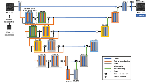
The proposed U-Net-based deep learning network is shown in Figure 1. This network is modified based on robust U-Net (RUNet) (Hu et al. 2019) structure, which consists of several number of convolutional layers, batch norm layers and activation layers using ReLU. Residual blocks (Lim et al. 2017) and pooling layers are used in the left path for down scaling of the input data. Some residual blocks of RUNet are removed to reduce the size of our model, which keeps two residual blocks for each down scaling layer. It shows the similar behavior to RUNet, which will be discussed in Results section. Low-resolution monochromatic images with resolution 128 × 128 pixel are upscaled using bicubic interpolation with factor 2 to adapt the input size of model. The output has the resolution of 256 × 256 pixel.

Figure 1. Proposed U-Net structure for super resolution

2.2. Content loss function

Unlike RUNet structure, content loss is involved for network training instead of perceptual loss. The content loss introduces pixel-wised loss besides pure perceptual loss. Since pixel-wised loss provides the benefit to the super-resolution image construction for its capability to match the pixel value globally (Lim et al. 2017), mean square error (MSE) loss is involved into the content loss with:

(1) $\begin{array}{c}{L}_{mse}\left(\hat{y},y\right)=\hspace{0.17em}\frac{1}{M}\sum _{i=1}^M{({\hat{y}}_i-\hspace{0.17em}{y}_i)}^2\end{array}$(1)

where M is total pixel amount of an image, while $\hat{y}$ and $y$ are predicted high-resolution images and target images.

Considering perceptual loss function showed good performance in super-resolution algorithm to enhance feature details in RGB images from low-resolution images (Johnson, Alahi, and Fei-Fei 2016), this loss function is involved for training procedure as a part of content loss. The perceptual loss function $\mathrm{\varnothing }\left(x\right)$ maps the predicted high-resolution images $\hat{y}$ and target images $y$ to the feature space and calculates the Euclidean distance between the prediction and target with:

(2) $\begin{array}{c}{L}_{perceptual}\left(\hat{y},y\right)=\hspace{0.17em}\frac{1}{N}\sum _{i=1}^N{[{\mathrm{\varnothing }}_i\left(\hat{y}\right)-{\mathrm{\varnothing }}_i\left(y\right)]}^2\end{array}$(2)

where N is the total pixel amount of the mapped image.

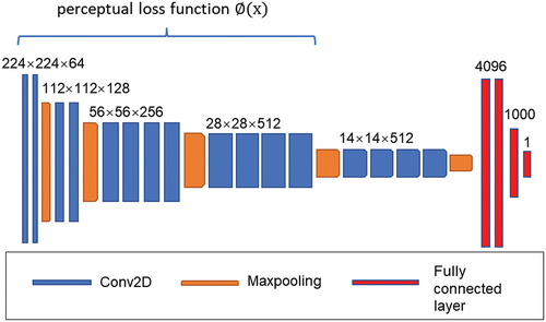
According to Simonyan and Zisserman (2014); Ledig et al. (2017), pre-trained VGG16- and VGG19-based classifier models are widely used for feature mapping, which showed improvement in SR algorithm in high-level image features. In this study, the pre-trained convolutional layers of VGG19 are used for getting perceptual loss. Since training procedure of VGG19 model used ImageNet database (Deng et al. 2009–2009) with RGB images, this model is not specific for AM monitoring images with monochrome images. To get perceptual loss, the monochrome image is repeated into 3 channels to adapt the input shape of pre-trained VGG19 classifier. The output of 3rd downscaling layer of VGG19 is used for perceptual loss function (Figure 2).

Figure 2. Perceptual loss function out of VGG19 network structure.

The content loss can be represented as follows:

(3) $\begin{array}{c}{L}_{content}=\hspace{0.17em}\lambda \times L_{perceptual}+L_{mse}\end{array}$(3)

where weight $\lambda$ of perceptual loss keeps the value of perceptual- and MSE-loss in the same order of magnitude. In this study, $\lambda =1/200$ is used for content loss, while to achieve high PSNR, $\lambda =0$ is set for using pure MSE loss.

2.3. Indicator for performance evaluation

Besides loss values of each network and loss function combination, behavior of image enhancement should be evaluated by a certain indicator with same range. Therefore, peak signal-to-noise ratio (PSNR) is presented as follows:

(4) $\begin{array}{c}PSNR=10lo{g}_{10}\left(\frac{MA{X}_I^2}{MSE}\right)\end{array}$(4)

where $MA{X}_I$ is the maximum pixel value of the image and MSE is the mean square error between the ground truth and the enhanced image, which is introduced in section 2.2. According to the hardware property, 8bit Bit-depth indicates $MA{X}_I$ with $2^8=255$. Higher PSNR indicates higher similarity between original image and enhanced image.

3. Experiment setup

The experiment setup for training and testing the proposed network structure for in-situ monitoring image enhancement is introduced in this section. A brief introduction of integrated monitoring system hardware for data acquisition on the LPBF machine is described firstly while the experiment design, while data generation and training detail are presented in the second step.

3.1. Hardware setup

As an in-situ monitoring system for LPBF process, an optical camera system is installed on EOS M290 with a high-resolution camera hr29050MFLGEC from SVS-Vistek GmbH, Germany. Property of the camera is shown in Table 1. To acquire high-resolution images for training procedure, the field of view (FoV) covers a small section with 180 × 120 mm on the build platform out of 250 × 250 mm using a lens of 120 mm focal length. The corresponding spatial resolution is $\frac{120\hspace{0.17em}mm}{4384\hspace{0.17em}pixel}=27\mu \mathrm{m}/\mathrm{p}\mathrm{i}\mathrm{x}\mathrm{e}\mathrm{l}$.

Table 1. Property of high-resolution camera.

Item	Value
Type of sensor	Charge-coupled Device (CCD) monochrome
Bit depth	8 bits
Sensor size	36.17 x 24.11 mm
Pixel size	5.5 x 5.5 µm
Resolution	6576 x 4384 pixel (29 Megapixel)
Exposure time	0.3s

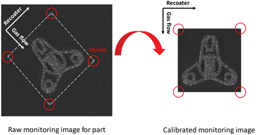
An illustration of the monitoring system setup is shown in Figure 3. To extent the optical path to fulfill focal length of camera system, a mirror was place on the process chamber. The working distance of this camera setup is around 550 mm from lens to building platform. A proximity switch is integrated into the machine and sent a layering signal during the re-coating process, when the re-coater reaches the switch. Monitoring images are taken after finish of laser exposure of each layer during LPBF process, which deliver the layer-wised surface information of the processed part. In addition, the acquired monitoring images are calibrated using the technique from (Z. Zhang 2000; zur Jacobsmühlen 2018), where a set of markers are printed around the printing objects and the position of the markers are extracted with individual objects after each printing to calculate the calibration matrix to compensate the perspective error and align the part orientation (shown in Figure 4). In this study, the calibrated image of each part has a resolution of 768 × 768 pixel.

Figure 3. Illustration of camera-based monitoring system setup.

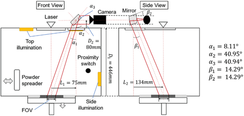
Figure 4. Raw monitoring layer images and its calibration.

3.2. Experiment design

Two different geometries with different laser parameters were designed and processed to get the monitoring images for training and test dataset. In this study, Sandvik 17–4PH stainless steel with particle size from 10 µm to 45 µm was selected. According to the property of the selected material and the engineering experience, the nominal settings of hatching distance (∆y_s), scan velocity (v_s) and laser power (P_L) were determined as reference parameter set (group 1 in Table 2). Then one of hatching distance and laser power was increased or decreased by 25% and 50%, generating different values of energy density ${\mathrm{E}}_{\mathrm{V}}=\frac{P_L}{d_s{v}_s\mathrm{\Delta }y{\hspace{0.17em}}_s}$, where $d_s\hspace{0.17em}$ is fixed laser beam diameter (shown in Table 2). The variation of ${\mathrm{E}}_{\mathrm{V}}$ can lead to different surface textures of the printed components, which have different details that need to be resolved and it can be used to enrich the dataset and test the performance of the neural networks. The geometries are shown in Figure 5. Due to stochasticity of LPBF process, micros defects, e.g. porosity and lack of fusion under 200 μm, cannot be generated manually at certain positions. Thus, Recognition of hatching distance ∆y_s which indicates the spacing of laser scanning path and has the similar size of micro defects, was the aim for the experiment. The whole print job contained in total 248 layers with layer thickness 30 μm, where the monitoring data from first 236 layers were used for training and data after the 236th layer were used for test.

Figure 5. Designed geometries for the experiment.

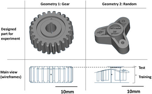
Table 2. Machine parameter configuration of experiment.

Material	Group	Geometry	Laser beam diameter ds [µm]	Scan velocity vs [mm/s]	Layer height Ds [µm]	Laser power PL [W]	Hatching Distance ∆ys [µm]	Volume Energy Ev [J/mm^3]	Comments
Sandvik 17–4PH	1	Gear	75	800	30	120	80	62.5	P0, H0, V0
	2	Gear	75	800	30	150	80	78.1	P0 + 25%, H0, V0
	3	Gear	75	800	30	180	80	93.8	P0 + 50%, H0, V0
	4	Gear	75	800	30	90	80	46.9	P0-25%, H0, V0
	5	Random	75	800	30	60	80	31.3	P0-50%, H0, V0
	6	Random	75	800	30	120	100	50.0	P0, H0 + 25%, V0
	7	Random	75	800	30	120	120	41.7	P0, H0 + 50%, V0
	8	Random	75	800	30	120	60	83.3	P0, H0-25%, V0
	9	Random	75	800	30	120	40	125	P0, H0-50%, V0

3.3. Data construction

The data construction follows the subsequent process, shown in Figure 6.

Figure 6. Data construction process.

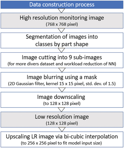
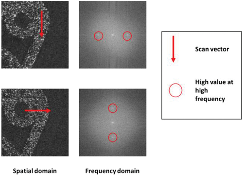
During LPBF process, powder bed image was taken by optical camera each time when a new layer was finished. Since on the one hand for each printing job a few parts with different geometries and parameter settings were printed at the same time, and on the other hand for each individual part the layer shape also varies along the build-up direction, images with different geometries and surface conditions can be collected within one printing job. However, since the goal of this study is to enhance surface textures of parts at each layer with image high frequency components (e.g. periodic strips of scan path) and help to recognize hatches, images in the dataset should have sufficient richness and generality in terms of geometries. Therefore, the collected raw images were firstly segmented after calibration into individual component images like gears, random shapes, etc. According to techniques used in (zur Jacobsmühlen 2018), each component image was further randomly cropped into 9 sub-images with the size of 256 × 256 pixels. The advantage of such method is twofold: on the one hand, in each sub-image only very simple geometries and small number of pixels are included, which offers the dataset more generality and reduces the workload for the neural networks. On the other hand, the random cropping acts as data augmentation, which enriches the dataset and reduces the possibility of overfitting for the algorithm. Thus, on cropped data, scan paths were visible on images in spatial domain and recognizable after 2D Fast Fourier Transformation (FFT) (in Figure 7).

Figure 7. Two cropped monitoring images and their Fourier transformation.

According to K. Zhang, Zuo, and L. Zhang (2018), low-resolution images can be generated by high-resolution image using downscaling and blurring. In this study, the high-resolution images were blurred by a mask, which approximates 2D Gaussian filter, with kernel 15 × 15 pixel and standard deviation of the distribution σ = 1.5, and then downscaled to 128 × 128 pixel. To adapt the input size of the model, the low-resolution image was up scaled to 256 × 256 pixel via bi-cubic interpolation. The detail of the image was removed visually on the processed images after down scaling, while high frequency components were removed in frequency domain using FFT (in Figure 8). The pair of low- and high-resolution images was used as input data for training the deep learning model. After the pre-processing, 26,950 pairs of input data for training procedure and 1017 pairs of test data, including more geometries, to evaluate performance for super-resolution model were generated.

Figure 8. Pair of low- and high-resolution images for model training and their frequency transformation.

3.4 Training details

The proposed super-resolution model was trained on a NVIDIA V100 GPU using the proposed dataset configuration. Input data for super-resolution model was divided into 80% for training and 20% as hold-out to monitor if the trained model is overfitted. Since these images are 8 bits, pixel values of high- and low-resolution images were normalized to [0,1] by dividing its maximum pixel value 255.

For evaluation of the performance of the proposed U-Net, SRCNN (C. Dong et al. 2016), SRResNet (Ledig et al. 2017), SRGAN (Ledig et al. 2017) and RUNet (Hu et al. 2019) were trained by the same configuration. In addition, MSE-, perceptual- and content-loss were applied for the training procedure. For each training procedure, the Adam optimizer was used with learning rate 0.001. The implementation is based on TensorFlow Keras.

4. Results

The experiment results are presented in this section, which contain training results of proposed U-Net model. The comparison with other network models is discussed in the second subsection while prediction failures are introduced in the last section.

4.1. Proposed U-Net model

The proposed U-Net model with MSE-, pure perceptual- and content-loss were trained for 50 epochs and reached the convergence of training losses (shown in Figure 9). PSNRs of training- and validation-set during the training procedure of the model are given with different losses as well. The results show that no overfitting occurred during the training process for any model. The model 2 with pure perceptual loss and pre-trained VGG19 led the model towards lower PSNR after several epochs, while loss continued decreasing during the training. From Table 3 it can be seen that model 1 (proposed model with MSE loss) gives the best PSNR result, while model 3 (proposed model using content loss) has the sub-optimal result.

Figure 9. Training procedure with training and hold-out loss and PSNR for proposed network with different loss functions

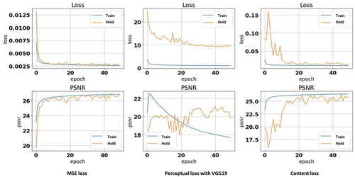
Table 3. Performance of proposed U-Net with different loss function.

Model number	1	2	3
SR method	Proposed U-Net	Proposed U-Net	Proposed U-Net
Loss function	MSE loss	Perceptual loss with VGG19	Content loss
Average PSNR of test set	28.7 dB	24.21 dB	27.24 dB

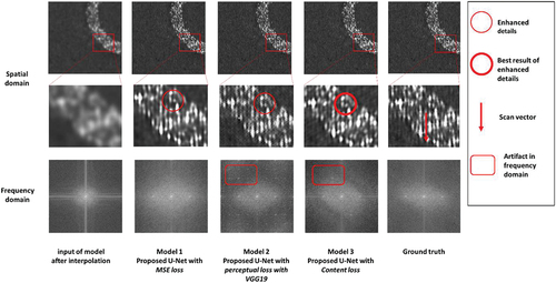
In Figure 10, the enhanced image results of the proposed U-Net with different loss functions are shown. In the upper part of the figure the complete output images are displayed. The lower part contains the partial enlarged image details and vertical laser scan paths are visible. The frequency representations are shown in the third line. From comparing the model outputs with their inputs, Model 3 (with content loss) enhanced the details of the laser exposed area and showed the visually sharp scan paths as displayed in the red circle. Model 1 with MSE loss enhanced the image globally. Model 2 resulted in an image enhanced with noise, since the pre-trained VGG19 model was not trained by LPBF monitoring data and not fully capable for single channel images. Considering their frequency representations after FFT, the proposed models can predict the high-frequency components, which were not involved in input data. However, artifacts (showed in red rounded rectangular) were generated in high-frequency section by perceptual loss and content loss as well, which can generate periodic artifacts on the images in spatial domain.

Figure 10. Enhanced image with proposed U-Net with different loss function and their frequency transformation.

4.2. Comparison with other networks

Results of comparable networks are shown in Table 4. Since model 7 (RUNet with VGG19 perceptual loss) was not capable due to overfitting, RUNet was trained by MSE loss as well (model 8). According to the comparison of results in Table 4, the proposed network (model 1 with MSE loss) shows better performance in PSNR compared to the other network structure. In addition, models using MSE loss (models 4, 5, 8) achieve the higher PSNR while models using perceptual loss and GAN-based structure (models 6,7) focused on texture level and had lower PSNR.

Table 4. Test result of Bicubic interpolation, SRCNN, SRResNet, SRGAN and RUNet.

Model number	-	4	5	6	7	8
SR method	Input	SRCNN	SRResNet	SRGAN	RUNet	RUNet
Loss function	-	MSE-loss	MSE-loss	Content loss+adversarial loss	Percep-tual loss	MSE-loss
Average PSNR of test set	23.9 dB	24.2 dB	28.4 dB	25.8 dB	4.46 dB	28.3 dB

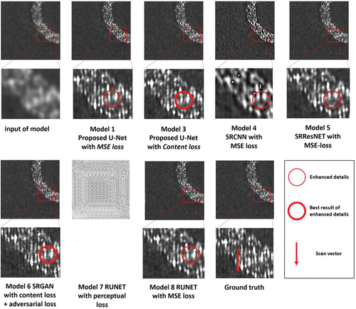
In Figure 11 the test output images of different network models are shown exemplarily. Except for SRCNN (model 4), the MSE loss-based networks (models 1, 5, 7) enhanced the high-frequency details visually on the exposed parts by reconstruction of scan paths in vertical direction. The proposed network with content loss (model 3) and SRGAN (model 6) provided visually the highest contrast detail.

Figure 11. Test result of proposed network, SRCNN, SRResNet, RUNET and SRGAN with different losses.

4.3. Prediction failure

Despite of the capability of improving the image quality, the content-loss-based (model 3) and GAN-based (model 6) SR models can also produce unplausible failure prediction. In Figure 12, for model 3 and 6, it is shown that the predicted vector orientation is different to the reality on ground truth, which are shown in the frequency domain accordingly.

Figure 12. Prediction failure by using content loss and SRGAN.

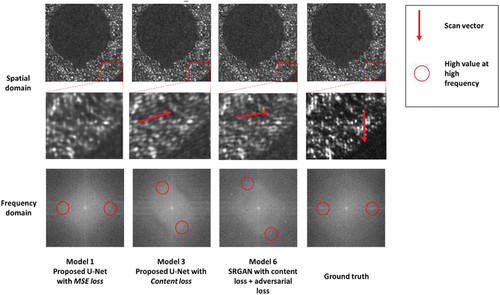
Scan vectors on the prediction result of the proposed MSE-loss-based network (model 1) are enhanced but visually not recognizable. In frequency domain values at high frequency area can still be distinguished, which is plausible to ground truth. In comparison the content loss function for proposed network (model 3) it differs by the pre-trained VGG19. As this is not specific for LPBF use cases it can map the low-resolution image into the wrong feature domain and lead to the fake feature prediction.

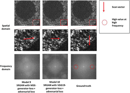
To examine the reason behind the fake prediction of SRGAN (Model 6), SRGAN was tested twice, splitting the content loss into its parts: SRGAN with pure MSE-loss for generator (Model 9) and SRGAN with pure perceptual loss for generator (Model 10). The result shows, that the change of the generator loss did not change the prediction behavior. The prediction procedure is driven by the generator-discriminator structure of GAN and fakes features. Further details can be seen in Figure 13. The dominant high values at high frequency section are hard to distinguished in predictions of Model 9 and Model 10.

Figure 13. Prediction by SRGAN with different generator loss.

4.4. Limitation

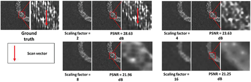
The proposed SR method shows the ability to enhance the low-resolution monitoring images by the factor of 2 and able to reconstruct the detailed features. To test the limitation of proposed method, three additional datasets were established using same high-resolution images in section 3.2, but with higher downscaling factors, which are shown in Table 5. Networks were trained using the same configuration in section 3.4. All training procedures were converged within 100 epochs. PSNRs of test datasets decreased with the increasing downscaling factor.

Table 5. Dataset for downscaling factor test.

Downscaling factor	Resolution of input image	Resolution of output image	Loss function	Amount of training set	Amount of test set	Average PSNR of test set
16	16x16 pixel	256 x 256 pixel	MSE	26950	1017	21.1 dB
8	32x32 pixel					22.4 dB
4	64x64 pixel					24.9 dB
2	128x128 pixel					28.7 dB

In Figure 14, an example of predictions using proposed network are shown using inputs with downscaling factors, 2, 4, 8 and 16. The scan vectors are recognizable from downscaling factor 4.

Figure 14. Predictions using inputs with different scaling factors.

5. Conclusion and outlook

In this study, a set of monitoring data was generated by experiments and pre-processed to fit the deep learning model training. The proposed U-Net model shows its capability to enhance the LPBF monitoring images and reconstruct details on the printed part surface by factor of 2. Proposed network structure with MSE loss shows the stable performance in PSNR indicator and frequency domain while content loss provides the possibility to draw the attention of training process to features. The prediction using content loss shows more detailed feature but can generate fake feature because the pretrained VGG19 network is not fully capable for additive manufacturing.

For future work, instead of using a pretrained VGG19 network for RGB images, a specific classifier or filter for LPBF needs to be designed and trained to map features of monitoring data properly. Besides, the current low-resolution and high-resolution image pairs cannot be fully used in the real situation since the low-resolution images are down scaled and blurred by a common kernel with the high-resolution images. To generate the real low-resolution images, a style transfer method should be considered. Furthermore, since the perceptual loss function maps the images to the feature domain and this deep-learning-based mapping procedure leads to the none-real predictions. Thus, an AM-specific feature mapping method needs to be considered.

Acknowledgments

Funded by the Deutsche Forschungsgemeinschaft (DFG, German Research Foundation) under Germany ́s Excellence Strategy – EXC-2023 Internet of Production – 390621612.

Disclosure statement

No potential conflict of interest was reported by the author(s).

Additional information

Funding

This work was supported by the Deutsche Forschungsgemeinschaft (DFG, German Research Foundation) under Germany ́s Excellence Strategy – EXC-2023 Internet of Production – 390621612.

References

- Agustsson, E., and R. Timofte. 2017. NTIRE 2017 Challenge on Single Image Super-Resolution: Dataset and Study. 2017 IEEE Conference on Computer Vision and Pattern Recognition Workshops (CVPRW). IEEE. 1122–1131. doi:10.1109/CVPRW.2017.150.
- Ali, U., Y. Mahmoodkhani, S. Imani Shahabad, R. Esmaeilizadeh, F. Liravi, E. Sheydaeian, K. Y. Huang, E. Marzbanrad, M. Vlasea, and E. Toyserkani. 2018. “On the Measurement of Relative Powder-Bed Compaction Density in Powder-Bed Additive Manufacturing Processes.” Materials & Design 155: 495–501. doi:10.1016/j.matdes.2018.06.030.
- Bee, L., S. Son, H. Kim, S. Nah, and K. M. Lee. 2017. “Enhanced Deep Residual Networks for Single Image Super-Resolution.” In 2017 IEEE Conference on Computer Vision and Pattern Recognition Workshops (CVPRW): IEEE.
- Berumen, S., F. Bechmann, S. Lindner, J.-P. Kruth, and T. Craeghs. 2010. “Quality Control of Laser- and Powder Bed-Based Additive Manufacturing (AM) Technologies.” Physics Procedia 5: 617–622. doi:10.1016/j.phpro.2010.08.089.
- Clijsters, S., T. Craeghs, S. Buls, K. Kempen, and J.-P. Kruth. 2014. “In Situ Quality Control of the Selective Laser Melting Process Using a High-Speed, Real-Time Melt Pool Monitoring System.” The International Journal of Advanced Manufacturing Technology 75 (5–8): 1089–1101. doi:10.1007/s00170-014-6214-8.
- Deng, J., W. Dong, R. Socher, L. Li-Jia, L. Kai, and L. Fei-Fei. 2009 - 2009. “ImageNet: A Large-Scale Hierarchical Image Database.” In 2009 IEEE Conference on Computer Vision and Pattern Recognition, 248–55: IEEE.
- Dong, C., C. C. Loy, H. Kaiming, and X. Tang. 2014. Learning a Deep Convolutional Network for Image Super-Resolution. Vol. 184–99. Cham: Springer. https://link.springer.com/chapter/10.1007/978-3-319-10593-2_13
- Dong, C., C. C. Loy, H. Kaiming, and X. Tang. 2016. “Image Super-Resolution Using Deep Convolutional Networks.” IEEE Transactions on Pattern Analysis and Machine Intelligence 38 (2): 295–307. doi:10.1109/tpami.2015.2439281.
- Everton, S. K., M. Hirsch, P. Stravroulakis, R. K. Leach, and A. T. Clare. 2016. “Review of in-Situ Process Monitoring and in-Situ Metrology for Metal Additive Manufacturing.” Materials & Design 95: 431–445. doi:10.1016/j.matdes.2016.01.099.
- Imani, F., A. Gaikwad, M. Montazeri, P. Rao, H. Yang, and E. Reutzel. 2018. “Layerwise in-Process Quality Monitoring in Laser Powder. Bed Fusion”.: American Society of Mechanical Engineers Digital Collection.
- Johnson, J., A. Alahi, and L. Fei-Fei. 2016. “Perceptual Losses for Real-Time Style Transfer and Super-Resolution”. In Computer Vision – ECCV 2016. B. Leibe, J. Matas, N. Sebe, and M. Welling edited by. Vol. 9906, 694–711.Lecture Notes in Computer Science 9906 Cham:Springer International Publishing.
- Ledig, C., L. Theis, F. Huszar, J. Caballero, A. Cunningham, A. Acosta, A. Aitken, et al. 2017. “Photo-Realistic Single Image Super-Resolution Using a Generative Adversarial Network.” In 2017 IEEE Conference on Computer Vision and Pattern Recognition (CVPR): IEEE.
- Marco, G., and B. M. Colosimo. 2017. “Process Defects and in Situmonitoring Methods in Metal Powder Bed Fusion: A Review.” Measurement Science and Technology 28 (4): 44005. doi:10.1088/1361-6501/aa5c4f.
- Michael, S., M. Merklein, D. Bourell, D. Dimitrov, T. Hausotte, K. Wegener, L. Overmeyer, F. Vollertsen, and G. N. Levy. 2017. “Laser Based Additive Manufacturing in Industry and Academia.” CIRP Annals 66 (2): 561–583. doi:10.1016/j.cirp.2017.05.011.
- Mohr, G. 2019. Measurement of Particle Emissions in Laser Powder Bed Fusion (L-PBF) Processes and Its Potential for in-Situ Process Monitoring. https://opus4.kobv.de/opus4-bam/frontdoor/index/index/docid/49387
- Mohr, G., S. J. Altenburg, A. Ulbricht, P. Heinrich, D. Baum, C. Maierhofer, and K. Hilgenberg. 2020. “In-Situ Defect Detection in Laser Powder Bed Fusion by Using Thermography and Optical Tomography—Comparison to Computed Tomography.” Metals 10 (1): 103. doi:10.3390/met10010103.
- Neef, A., V. Seyda, D. Herzog, C. Emmelmann, M. Schönleber, and M. Kogel-Hollacher. 2014. “Low Coherence Interferometry in Selective Laser Melting.” Physics Procedia 56: 82–89. doi:10.1016/j.phpro.2014.08.100.
- Plessis, D., Anton, I. Yadroitsev, I. Yadroitsava, and S. G. Le Roux. 2018. “X-Ray Microcomputed Tomography in Additive Manufacturing: A Review of the Current Technology and Applications.” 3D Printing and Additive Manufacturing 5 (3): 227–247. doi:10.1089/3dp.2018.0060.
- Robinson, J., I. Ashton, P. Fox, E. Jones, and C. Sutcliffe. 2018. “Determination of the Effect of Scan Strategy on Residual Stress in Laser Powder Bed Fusion Additive Manufacturing.” Additive Manufacturing 23: 13–24. doi:10.1016/j.addma.2018.07.001.
- Simonyan, K., and A. Zisserman. 2014. “Very Deep Convolutional Networks for Large-Scale Image Recognition.“ arXiv preprint arXiv:1409.1556.
- Spears, T. G., and S. A. Gold. 2016. “In-Process Sensing in Selective Laser Melting (SLM) Additive Manufacturing.” Integrating Materials and Manufacturing Innovation 5 (1): 16–40. doi:10.1186/s40192-016-0045-4.
- Spierings, A. B., K. Dawson, M. Voegtlin, F. Palm, and P. J. Uggowitzer. 2016. “Microstructure and Mechanical Properties of as-Processed Scandium-Modified Aluminium Using Selective Laser Melting.” CIRP Annals 65 (1): 213–216. doi:10.1016/j.cirp.2016.04.057.
- Tai, Y., J. Yang, X. Liu, and X. Chunyan. 2017. “Memnet: A persistent memory network for image restoration.“ In Proceedings of the IEEE international conference on computer vision (pp. 4549–4557). IEEE. doi:10.1109/ICCV.2017.486.
- Tatsuaki, F., T. Ueda, M. R. Alkahari, and A. Hosokawa. 2013. “Investigation of Laser Consolidation Process for Metal Powder by Two-Color Pyrometer and High-Speed Video Camera.” CIRP Annals - Manufacturing Technology 62 (1): 223–226. doi:10.1016/j.cirp.2013.03.032.
- Xiaodan, H., M. A. Naiel, A. Wong, M. Lamm, and P. Fieguth. 2019. “RUNet: A Robust UNet Architecture for Image Super-Resolution.” In 2019 IEEE/CVF Conference on Computer Vision and Pattern Recognition Workshops (CVPRW): IEEE.
- Zenzinger, G., J. Bamberg, A. Ladewig, T. Hess, B. Henkel, and W. Satzger. 2015. “Process monitoring of additive manufacturing by using optical tomography.“ In AIP Conference Proceedings (Vol. 1650, pp. 164–170). AIP Publishing LLC
- Zhang, Z. 2000. “A Flexible New Technique for Camera Calibration.” IEEE Transactions on Pattern Analysis and Machine Intelligence 22 (11): 1330–1334. doi:10.1109/34.888718.
- Zhang, K., W. Zuo, and L. Zhang. 2018. “Learning a Single Convolutional Super-Resolution Network for Multiple Degradations.“ Proceedings of the IEEE conference on computer vision and pattern recognition (pp. 3262–3271). IEEE. doi:10.1109/CVPR.2018.00344.
- Zhihao, W., J. Chen, and S. C. H. Hoi. 2021. “Deep Learning for Image Super-Resolution: A Survey.” IEEE Transactions on Pattern Analysis and Machine Intelligence 43 (10): 3365–3387. doi:10.1109/TPAMI.2020.2982166.
- Zur Jacobsmühlen Joschka. 2018. Image-based methods for inspection of laser beam melting processes. RWTH Aachen University. http://publications.rwth-aachen.de/record/760489