A stochastic evaluation framework to improve the robustness of manufacturing systems

ABSTRACT

This work presents a framework to assess the robustness of manufacturing systems. Robustness, which is an indicator of the system’s ability to maintain its desired performance in face of disturbances, is quantified considering the variance of manufacturing system performance indicators. According to the framework, key objectives are first explicitly defined to guide a thorough exploration of the manufacturing system structural and dynamic characteristics. Several simulation experiments, orchestrated methodically through experimental design, are run and statistically analysed through analysis of variance (ANOVA) tests, including also financial implications. The framework has been tested and validated against a case study where the robustness of the manufacturing system with regard to six aerospace product types is evaluated. The mentioned case study proved that the framework has the potential to improve the robustness of manufacturing systems, identifying the most and least disruptive dispatching policies.

KEYWORDS:

• Robustness
• manufacturing systems
• discrete event simulation
• applied statistics
• system simulation

1. Introduction

Typically, manufacturing systems are designed apriori to be able to absorb certain levels of disturbance (Klibi, Martel, and Guitouni 2010). The occurrence of these disturbances, often uncertain, could potentially entail adverse impact on the performance of the manufacturing system. Disturbances are disruptions to plans comprising a cause and an effect, resulting in a significant deviation from the expected result (Chryssolouris 2006). Disturbances to a manufacturing system can be unforeseen or unintended and have an undesirable impact on cost, time and quality. For a review of the possible disruptions, and mitigating techniques in the context of production systems and supply chains, a good overview is provided by Tobias, Lange, and Glock (2020).

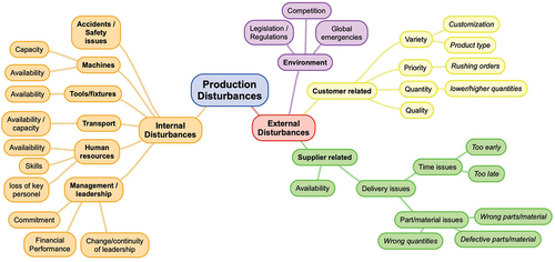
To mitigate the potential impacts of these disturbances, manufacturing systems often incorporate measures to adapt in the face of such disturbances. These could be classified as internal or external, as illustrated in Figure 1 (Saad and Gindy 1998), but this categorisation can be further expanded to reflect current trends. Internal disturbances, occurring within the boundaries of the manufacturing system, include equipment failure, faulty products, variations in processing times and transportation network failure (Adenso-Díaz, Mar-Ortiz, and Lozano 2018) amongst others. On the other hand, external disturbances occur within the wider supply chains and include typical examples like unexpected spikes in demand or suppliers’ breach of agreements, amongst others.

Figure 1. Classification of disturbances. Expanded from Saad and Gindy (1998) to include current trends.

In light of these varied sources of disturbance, a manufacturing system that can continue to preserve its performance at an acceptable level is said to be robust (Efthymiou et al. 2018). As disturbances have been classified as internal and external, robustness, that protects against such disturbances, has been classified as either passive or active (Telmoudi, Nabli, and Radhi 2008). Passive robustness is demonstrated in a manufacturing system’s ability to deal with disturbances without any modifications to the system’s control parameters (inputs). This type of robustness is often incorporated in a manufacturing system’s design phase allocating additional redundant capacities. Active robustness, on the other hand, is demonstrated when a manufacturing system responds to disturbances through modifications of its control parameters. Similar to the aforementioned classification, manufacturing systems robustness can be achieved in two approaches: proactive and reactive (Colledani et al. 2016). The proactive approach aims at establishing a sub-optimal configuration of the line to deal with future issues via overcapacity and redundancies without further changes. The reactive approach, instead, aims at acquiring the skills to react immediately to changes, such as rescheduling or taking advantage of modularity. To explain more, in order to enhance the robustness of a manufacturing system, multiple measures can be taken. One approach is redundancy (Kamalahmadi, Shekarian, and Mellat Parast 2022), which implies the availability of an additional, exact element that fulfills the same function. Stocking raw material or having an additional machine tool (such as a lathe or a milling machine) are common examples. On the other hand, functional redundancy is the existence of a different element able to perform the same function (Meyer 2016). A computer numerical control machine that can perform different operations provides functional redundancy (CNC turning or machining centres), and additive manufacturing machines (‘3D printers’) are common examples of functional redundancies enablers. Both redundancies enable routing flexibility, providing breakdown tolerance and increasing robustness.

To mitigate the potential adverse impacts of disturbances, measures to enhance robustness are usually incorporated into a manufacturing system prior to its establishment (i.e. at the design stage). This is manifest in design decisions at different planning horizons, such as facility layout and scheduling decisions. Facility layout decisions are considered strategic; hence, they impact the long-term performance of a manufacturing system and are often costly to reverse. Facility layout decisions include determining the optimal, or near optimal, location of resources such as machines and assembly lines in a manufacturing system (Drira, Pierreval, and Hajri-Gabouj 2007). Papers that review the literature in facility layout problem with respect to robustness include the work of Kulturel-Konak (2007) as well as Meller and Gau (1996) where the authors survey the literature and classify different problems and solutions related to the design of a robust and flexible facility to cope with uncertainty. Scheduling, on the other hand, falls under short-term, or operational decisions and, therefore, these decisions can be reversed relatively easily with less severe consequences than those of strategic nature. Scheduling decisions deal with allocating resources to tasks (Pinedo 2016), such as allocating jobs to machines. Scheduling decisions in a robust manufacturing system context are also important as disturbances, such as machine breakdown, might require rescheduling of an entire system’s operations to compensate for the missing resource. Sabuncuoglu and Goren (2009) provide a scheduling decision taxonomy examining the different approaches to achieve operational robustness and stability. They start defining the appropriate scheduling mode and time in different situations, giving insights about the different disturbances and respective responses.

To cope with the uncertainty that results in disturbances to production plans, rolling horizon practices are usually adopted to reduce uncertainty. Such practices include updating periodically both push-based supplying and production plans to guarantee components and raw materials availability. These practices can stress the supply chain as scheduling is constantly changed. Tolio, Urgo, and Váncza (2011) propose a robust approach to predict and react to sudden events by identifying maximum lateness as an objective function to minimize. This considers not only the average occurrences but also the worst cases to cover the complete range of possibilities. The final aim is to keep planning simple and avoid disruption propagation, introducing the financial concept of risk. Hence, the authors provide the ‘Value at risk’ (VaR) and ‘Conditional Value at Risk’ (CVaR) functions, to calculate the job tardiness as a scheduling probability distribution, establishing a significance level ($\alpha$) to determine the final loss. (Tolio, Urgo, and Váncza 2011)

To quantify robustness in manufacturing systems, an evaluation framework was introduced by Efthymiou et al. (2018) providing a mathematical definition of robustness and identifying relevant uncertain parameters. In such framework, the different scenarios against which the system has to be tested and its stability evaluated are defined based on the different input parameters that affect the system. Subsequently, simulations are run to estimate the manufacturing system performance in the mentioned scenarios. Finally, data post-processing, such as distribution fitting to identify the parameters and probability estimation to establish the robustness threshold, are performed. Building on this work, Pagone et al. (2019) evaluated robustness devising a Design of Experiments (DoE) of 18 scenarios based on a ‘one time at factor’ design of three disturbance elements: assembly time, rework time and rework occurrence, and three dispatching rules: First In First Out (FIFO), Shortest Processing Time (SPT) and Earliest Due Date (EDD). A limit is set to define the robustness of the system and the scenarios are listed and compared to understand how the disturbances and the different policies affect system stability. In addition to the aforementioned approach, a multi-level framework was developed by Stricker et al. (2015) to assess manufacturing system robustness in order to tackle its disturbances and improve capacity planning, scheduling and management decisions. Also, Adane et al. (2019) review the employment of system dynamics simulation tools in the modelling and decision-making in the context of robust manufacturing systems. A heuristic (genetic algorithm) was combined with Petri Nets in decision-making with regard to the design of robust manufacturing systems by Sharda and Banerjee (2013). Petri Nets, integrated with agent-based modelling, have also been used by Blos, da Silva, and Ming Wee (2018) for the design of disruption management plans in the context of supply chain and production systems. Tsiamas and Rahimifard (2021) developed a model-based decision-support system that can be employed in a wide array of disruption scenarios but it was mainly targeted at external disruptions caused by factors outside a manufacturer’s control (e.g. political and climate change-related disruptions). Yuchen, Zixiang, and Saldanha-da-Gama (2021) developed an optimization model that minimises the total cost addressing the assembly line balancing problem in the face of disruptions. Such model includes multi-period modelling as well as the stochastic nature of disruption rates and processing times but it is limited in its applicability only to assembly line balancing. Furthermore, Zanchettin (2022) developed a robust simulation and control-based dispatching and scheduling method in a make-to-order production environment against production time variability. This approach integrates digital twin technology and minimises the deviation from a reference production schedule but it would be challenging to apply at strategic decision level. Chen et al. (2022) improved a method previously published by Thürer et al. (2012) to increase robustness against bottlenecks and variability of resources by developing an advanced order release. Traditional dispatching rules were compared to the advanced one using discrete-event simulations to show the benefits on the system robustness. Although valuable, the proposed approach is designed to work only at an operational level and does not provide insights into the driving factors that affect robustness that only a deeper statistical analysis (e.g. ANOVA) can provide. The ability to identify the factors at the root of disruptions is part of the framework proposed in this work.

In summarising the mentioned numerous approaches to robustness in the scientific literature, there is an important (and broad enough) trait that can be used to classify them: their applicability to strategic, operational level or both (Table 1). It can be noted that the definition used to build the framework proposed in this work (i.e. the ‘stochastic’ definition) is one of the few that can be applied with maximum generality.

Table 1. Classification of robustness approaches available in the open literature based on the extent of applicability. SD: system dynamics: GA: generic algorithms; PN: petri networks; AB: agent-based; MTO: Make-To-Order.

Approach to Robustness	Strategic level	Operational level	Reference
Active		x	(Telmoudi, Nabli, and Radhi 2008)
Passive	x		(Telmoudi, Nabli, and Radhi 2008)
Pro-active		x	(Colledani et al. 2016)
Reactive	x		(Colledani et al. 2016)
Item redundancy	x		(Kamalahmadi, Shekarian, and Mellat Parast 2022)
Functional redundancy		x	(Meyer 2016)
Layout focussed	x		(Kulturel-Konak 2007; Meller and Gau 1996)
Scheduling		x	(Sabuncuoglu and Goren 2009)
Minimisation lateness	x	x	(Tolio, Urgo, and Váncza 2011)
Stochastic	x	x	(Efthymiou et al. 2018)
Multi-level		x	(Stricker et al. 2015)
SD simulation	x	x	(Adane et al. 2019)
GA and PN simulation	x		(Sharda and Banerjee 2013)
AB and PN simulation		x	Yuchen, Zixiang, and Saldanha-da-Gama (2021)
Supply chain		x	(Tsiamas and Rahimifard 2021)
Assembly line balancing		x	Rakesh et al. (2000)
Time variability in MTO		x	(Zanchettin 2022)
Optimal order release		x	(Chen et al. 2022)

Since some types of disturbances are unavoidable and difficult to predict, and since hedging against all types of disturbances is generally deemed an impossible task (Rakesh et al. 2000), manufacturing systems should incorporate measures to establish and maintain robustness. In order to achieve this, a logical prerequisite is to develop a thorough understanding of robustness, and subsequently devise methodical approaches to evaluate it. In the next section, several definitions of robustness from different perspectives are provided, followed by the robustness evaluation framework.

The main contribution to knowledge of this work lies in the methodology underpinning the mentioned framework that is able to evaluate the robustness of manufacturing systems against any type of disturbances on any chosen performance metrics, with a detailed, step-by-step, methodical approach. A collection of appropriate tools and approaches that span several disciplines comprising engineering, operational research and statistics, combined in a unified framework make this work unique to the knowledge of the authors. Finally, this paper illustrates the applicability and effectiveness of the framework with a real-world case study applied to a UK aerospace manufacturing facility. Such case study does not aim at providing a comprehensive overview of disturbances in manufacturing systems, but only to show the efficacy and effectiveness of the framework.

2. Robustness and evaluation framework

2.1. Definition of robustness

Multiple definitions and parallelisms exist around the term manufacturing systems robustness while, as Efthymiou et al. note, a comprehensive definition is absent (Efthymiou et al. 2018). Multiple authors defined manufacturing systems robustness from different standpoints. Stricker and Lanza provide different definitions and drew parallelisms between the concept of robustness and other similar terms, such as flexibility, agility, risk and resilience (Stricker and Lanza 2014). Furthermore, they provide a general definition of robustness as the system’s ability to maintain its desired service level in the face of disturbances (Stricker and Lanza 2014). Alderson and Doyle characterise a manufacturing system as robust if its performance is invariant to different sets of perturbations (Alderson and Doyle 2010). Another definition was provided by Telmoudi et al. as the aptitude of a system to preserve its specified properties against foreseen or unforeseen disturbances (Telmoudi, Nabli, and Radhi 2008). Robustness has also been defined as the ability to reach the Key Performance Indicators (KPIs) levels in face of disturbances (Colledani et al. 2016). Formally, a quantitative definition used in this work is obtained by establishing first a limit $L$ for each KPI that should not be exceeded when a function representing the manufacturing system $f$ is evaluated according to operating conditions $S$ (Equation (1)(1) $f(S)\le L,$(1) ) (Efthymiou et al. 2018). Thus, considering the stochastic nature of real systems, the robustness function $f$ is evaluated as the probability that the confidence interval half-width verifies Equation (2)(2) $F(L)=Pr(f(S)\le L),$(2) (Efthymiou et al. 2018).

(1) $f(S)\le L,$(1)

(2) $F(L)=Pr(f(S)\le L),$(2)

2.2. Framework to evaluate robustness

The framework encapsulates the methods presented by Efthymiou et al. (2018) and Pagone et al. (2019) significantly widening the extent of the analysis with a rigorous, full factorial design of the experiment and a systematic data analysis (Figure 2). The aim to quantitatively evaluate the robustness of manufacturing systems against disturbances is achieved with three consecutive phases: manufacturing system audit, experimentation and data analysis.

Figure 2. Robustness evaluation framework.

In the audit phase, the manufacturing system is first defined where its entities, parameters and their values are identified. To achieve this aim, first the system is analyzed through a thorough exploration of its structural and dynamic characteristics. Structural characteristics refer to the resources that constitute the manufacturing system and their capacities. Resources include, but are not limited to, machines (such as lathes and milling machines), operators (where their skill levels are noted) and warehouses (and their capacities). Dynamic characteristics, on the other hand, are the attributes of the manufacturing system at product level. Such characteristics include, but are not limited to, product routings and cycle and setup times. The next step within the manufacturing system audit phase is the identification of the operating conditions, potential disturbances and uncertainties. In general, this step could be perceived as the development of scenarios where different values that the dynamic characteristics can take are investigated and noted. Potential disturbances and uncertainties, both internal (such as probability of rework) and external (such as supplier delays) are also explored in this stage. A collection of certain values for different parameters (e.g. high demand, long supplier lead time, high probability of rework, etc.) constitute a scenario. The first phase of the framework is achieved mainly through close observation of the manufacturing system. In particular, field visits and structured interviews with stakeholders at different levels are required in order to develop a clear and thorough understanding and, subsequently, analyse it properly. There are, however, challenges associated with the successful implementation of this phase; mainly capturing uncertainty. To explain more, if disturbances, to a certain extent, can be predicted in nature (e.g. fluctuating demand, machine breakdown, faulty products that need rework etc…), then it is not necessarily the case with regard to the magnitude, probability of occurrence and the impact of such disturbances on the system. Furthermore, metrics affected by the disturbances and related to quality or cost (for example) may be audited and considered in the further steps without restricting the validity of the analysis.

The second phase of the framework is the experimentation that revolves around a Discrete Event Simulation (DES) model imitating the operations of the manufacturing system. The choice of a DES model might seem restricting considering that there are other useful manufacturing systems simulation approaches. Broadly speaking, simulation modelling can be divided into two categories according to the time advancement mechanism: continuous and discrete (Law 2015). Under these two broad categories, three mainstream simulation approaches lie: system dynamics, discrete-event and agent-based. There is a plethora of literature – e.g. Siebers et al. (2010); Maidstone (2012); Sumari et al. (2013); Kin et al. (2010) – that explains and compares each of these mainstream simulation approaches, their time advancement mechanisms, their capabilities of handling uncertainties, abstraction level and suitability of modelling different industrial settings, among other attributes. Therefore, considering the purpose of investigating through simulation the performance of manufacturing systems in the face of disturbances (robustness) under uncertainty, it is deemed that DES is the appropriate modelling approach to use to achieve this goal. However, it might be correctly argued that agent-based modelling can be equally appropriate; it should be noted that an agent-based approach can be considered as a special case of DES because it uses the same time advancement mechanism (Law 2015). Therefore, agent-based modelling could be profitably used in this framework as a substitute of DES when it offers a clear advantage – typically, in the investigation of complex emerging behaviour, stemming from a distributed system (Borshchev and Filippov 2004).

In the simulation model development step of the experimentation phase, the model’s aim, contents, inputs, outputs and assumptions are prepared. This is a particularly subtle task as a balance has to be carefully established between complexity (i.e. modelling many processes and accounting for a large number of disturbances) and simplicity (modelling and accounting for only key processes and disturbances with minimal impact on the model’s accuracy). In this step, data collected in the previous phase of the framework will be used to feed the simulation model. Deterministic data (e.g. layout parameters, product types, etc…) and stochastic data (probability distributions for cycle and setup times, demand profiles, etc…) will be used to build and experiment with the model. In order to effectively examine the robustness of the manufacturing system, multiple scenarios have to be investigated through simulation (e.g. high probability of product failure coupled with high cycle time and high demand). This step is different from the ‘Operating conditions, potential disturbances and uncertainties identification’ in the first phase. The difference is that in this step, an assortment of scenarios is selected to be simulated in order to reflect possible disturbances and subsequently evaluate robustness, while in the first phase a comprehensive list of scenarios is developed and are not necessarily all included in the experimentation. The selection of the assortment of scenarios is a step referred to as the Design of Experiments (DoE). The DoE for the evaluation framework is factorial DoE; meaning that, unlike the ‘one at a time’ DoE approach, the impact of the interaction between different factors is investigated through the experiments. To accomplish this step, the factors that their variation impacts the outcome of the system and the levels, which are the values that these factors can take in the experiments have to be identified. Identifying the experimental factors and the levels will then determine the number of scenarios to be examined.

Since the simulation model is stochastic, one simulation run does not provide statistical representativeness and, in turn, meaningful insight about the modelled manufacturing system. Therefore, multiple simulation replications (each containing independent random values for the stochastic parameters) drawn from probability distributions have to be performed. These simulation replications constitute samples from all possible scenarios (i.e. the entire population of scenarios). Then, after performing a number of simulation replications, the mean values for the desired outcome can provide a more representative insight into the performance of the system. To determine the minimum required number of simulation replication, the confidence interval method is employed in the robustness evaluation framework (Montgomery 2017). The confidence interval method provides a statistical means to indicate how accurate the mean of the required performance metric is being estimated (Robinson 2004). To explain more, the confidence interval ($CI$) is calculated as

(3) $CI=\bar{F}(L)\pm t_{n-1,\alpha /2}\frac{\sigma }{\sqrt{n}},$(3)

$\bar{F}(L)$ is the mean of the simulation output, $t_{n-1,\sigma /2}$ is the Student’s $t$-distribution with a degree of freedom $n-1$ and significance level $\alpha /2$, $\sigma$ is the standard deviation and $n$ is a sufficiently large number of replications. The significance level ($\alpha$) refers to the probability that the true mean (the output of the simulation model for the desired performance metric if the simulation is run for an infinite number of replications) falls outside the desired confidence interval ($1-\alpha$). The application of the confidence interval analysis serves not only with the determination of the number of simulation replications but also provides an indication about the degree of variance within the manufacturing system. To explain more, if the output of the simulation model is relatively stable (i.e. low variance observed among replications), then the number of simulation replications determined by applying the confidence interval method will be low. Alternatively, if the outcome is unstable (i.e. high variance observed among replications), then this is an indication that the manufacturing system is prone to disturbances and subsequently a higher number of simulation replications will be required to level out the cumulative mean within a sufficiently narrow confidence bounds.

The final phase of the framework, i.e. the data analysis phase, takes place after the discrete-event simulation model is developed, the scenarios to be investigated identified and several simulation replications are performed. The data analysis phase consists of two distinct steps: analysis of variance (ANOVA) and the financial performance estimation. The former, which is twofold (within individual scenarios and among different scenarios), provides a means to quantitatively examine the variance in the obtained sample means through different statistical tests. The latter provides a means to estimate the impact of different disturbances on financial metrics. Such metrics could be different economic indicators like inventory operators’ costs, among others. Similar to the simulation model, the nature of the data analysis phase depends on the nature of the manufacturing system and the disturbances being investigated. Therefore, due to the models being relatively context-dependent, each application of the framework will have its own unique features, operating inside a context-independent framework.

Finally, it should be noted that the framework can work effectively with re-entrant data flows (i.e. iteratively) at any stage of its execution providing closed-loop optimisation opportunities to the user (e.g. re-evaluation after improvement).

3. Case study

3.1. Specifications and manufacturing system audit

To validate and test the robustness evaluation framework, it has been applied to a case study with the production of six different aircraft’s heat exchangers. The presented case study does not aim at showing a complete picture of disturbances in manufacturing systems, but only illustrate the validity and usefulness of the framework in a real-world scenario.

The product routing, which is shared among the six part types, is depicted in Figure 3 showing ‘high-level’, key production steps.

Figure 3. High-level product routing.

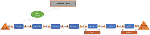
The production process begins when an order is released followed by kitting and assembly (performed by kitters and assemblers, respectively). The next stage is machining, which consists of three consecutive steps: turning with lathe one, turning with lathe two and milling. These processes are conducted by several machinists with different skill levels, which increases the variability of the process in terms of cycle time and the probability of the need to rework. After milling is completed, an inspection at an Air-Under-Water (AUW) station is conducted to test the quality of the produced part and determine whether any rework is required. If a part fails the AUW inspection, a rework is conducted until it passes the inspection.

Following the framework depicted in Figure 2, the structural characteristics of the framework can be identified as the resources used in the production of parts, which are the lathes and milling machines and the operators performing various production activities. The dynamic characteristics, however, contain the products routing, which are depicted in Figure 3 and cycle and setup times. The next step in the first phase is to identify the operating conditions, disturbances and uncertainties. The operating conditions that will be investigated are the dispatching rules which could be First In First Out (FIFO), Earliest Due Date (EDD) and Shortest Processing Time (SPT). External factors, such as demand profiles and suppliers lead time will be incorporated into the simulation model along with the uncertainties associated with their values. After examining the manufacturing system, through field visits and interviews with stakeholders of different levels directly involved in the production processes, the following key disturbances (and the uncertainties associated with them) were determined: assembly time variability, rework time variability and probability of rework.

3.2. Virtual experimentation

3.2.1. Discrete-event simulation model

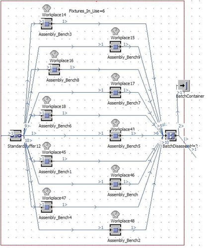
During this phase of the framework, the discrete-event model is developed to create a virtual environment, representing the manufacturing system, to investigate different scenarios with. The simulation model, which was developed in Tecnomatix Plant Simulation (a commercial discrete-event simulation platform), runs the production process depicted in Figure 3. During each simulation replication, the variability of disturbances is calculated rescaling probability distributions by the solution of small systems of equations calling an external numerical tool coded in Modern Fortran (Pagone et al. 2019). Figure 4 below depicts a snapshot of the simulation model’s Assembly processes.

Figure 4. Snapshot from the simulation model depicting the Assembly processes, one part of the entire discrete simulation model.

To incorporate the stochastic nature of the manufacturing system into the simulation model, past data (identifying uncertainties in phase 1) of processing times and probability of reworks was analysed and fitted to triangular probability distributions deemed the most suitable to the nature of the processes modelled and the relevant data available. The three parameters that the triangular distribution takes are: minimum, maximum and most likely (i.e. the mode).

3.2.2. Design of experiments

After the simulation model has been developed and validated, the next step in the experimentation phase is to systematically devise scenarios to investigate through DES based on Design of Experiments (DoE). These scenarios typically represent different operating conditions (factors) which, for the purposes of this case study, were determined to be dispatching rules. The selection of dispatching rules is case specific, meaning that any other operating conditions could be investigated. Typically, what dictates the nature of factors in a DoE experiment is the overall aim of the framework’s application, which in this case is the evaluation of the robustness of the manufacturing system under different dispatching rules. The dispatching rules included in the DoE are, as stated earlier, FIFO, EDD and SPT. The levels of disturbances that are included in the DoE are twofold: low (which reflects the normal operations with slight expected variations) and high (which reflect potential disruptive high variation). These levels of disturbances were devised based on the data collected, and close interaction with stakeholders directly involved in operating the manufacturing system. To represent these two levels of disturbances in the DoE, the low level of disturbance is represented by the mode (most likely) values observed from the collected data. The high disturbance level is determined, after observing all extreme data points and soliciting the opinions of those operating the manufacturing system, to be represented by increasing the coefficient of variation (standard deviation to mean ratio) by 20% of its original value. Due to the small number of levels (low and high disturbances) and factors (FIFO, EDD and SPT), a full factorial DoE is possible for this case study. The number 2 represents the level of disturbances (low and high), while the exponent k represents the factors (i.e. 3). Therefore, a total of 8 scenarios will be run in the simulation model as shown in Table 2 below where Scenario A refers to the ‘as-is’ scenario. Each of these eight scenarios will be run for a number replications determined through confidence interval analysis.

Table 2. Case specifications of full factorial design of experiments.

Scenario	Assembly time	Rework time	Rework
identifier	variability factor	variability factor	probability factor
A	1	1	1
B	1.2	1	1
C	1	1.2	1
D	1.2	1.2	1
E	1	1	1.2
F	1.2	1	1.2
G	1	1.2	1.2
H	1.2	1.2	1.2

3.2.3. Confidence interval analysis

The aim of the confidence interval analysis is to determine the minimum number of simulation replications for each of the scenarios presented in Table 2. Several simulation replications are required, as stated earlier, to produce meaningful output as the simulation model is stochastic and therefore the mean of several replications is more representative of the actual system. The desired confidence interval has been set at 95% since increasing it further will require many more replications and will contribute to only marginal increases (i.e. slight tightening to the confidence bounds). The KPIs of choice, as advised by managers, are related to lead times and average tardiness.

After observing the confidence bounds for the selected KPIs over several simulation replications (exemplified by Figure 5 for Scenario B, i.e. disturbance in assembly time variability under EDD dispatching rule), the number of replications has been set at 300. This is because, although the set significance level is often met well before 300 replications, it has been observed that this value offers enough margin to cover also the occurrence with more extreme output (Robinson 2004). Therefore, as a general statement, it is advised to continue performing several more replications after the desired significance level has been met. This reasoning will be further clarified with numerical evidence in Section 4 (i.e. Results and discussion).

Figure 5. Sample significant level for Scenario B under EDD dispatching rule with the increase of number of simulation replications.

3.3. Data analysis

3.3.1. ANOVA analyses

To analyze the system variability and provide reliable statistics to improve robustness, two different ANOVA have been conducted. The first one, between scenarios evaluates the effects of disturbances onto the system, while the latter, within each scenario, aims at determining the best dispatching rule to cope with the disturbances themselves. Generally speaking, ANOVA provides a more detailed understanding of a phenomenon underlying variance by decomposing the observed overall variance into contributions by sources of variation (i.e. ad-hoc defined groups) (Zhao, Shifu, and Yoshikawa 2013; Barbé, Van Moer, and Rolain 2009).

The ANOVA between scenarios grouped data according to each scenario and run a series of tests. Firstly, a normality test of groups using quantile-quantile (qq) plots was performed, followed by the fit of an ANOVA model on the data and the analysis of the residuals obtained (calculation of their skewness and kurtosis and Cook’s distance to detect possible outliers). Then, the homogeneity of variances was checked by Bartlett’s test and, since the homogeneity was never observed, Welch’s $t$-test (particularly reliable for unequal variances) was performed. A final, pairwise comparison of group means was performed by Games-Howell post-hoc test that does not assume equal variances. The subsequent ANOVA within each scenario grouped data for each KPI according to the dispatching rules, i.e. the same disturbances were dictated for the same KPI. For this reason, the previously observed problem homogeneity of variances is not present in this analysis (when performing Bartlett’s test) that followed the same procedure previously described where (appropriately) Turkey’s test substituted Games-Howell one.

Both ANOVA were implemented in R programming language.

3.3.2. Financial implication estimate

An estimate of financial implications was devised to further compare different dispatching rules (i.e. FIFO, EDD and SPT) from an economic standpoint. The most turbulent conditions (those in Scenario H) were assumed as benchmark where rework likelihood disturbance was set at maximum level over the replications (set at 300) per policy to get a robust system. The model assumptions are:

• The system is labour intensive; hence, the focus will be the reduction of working hours and their translation in monetary or alternative resources.

• The comparison is between the current system (using FIFO) and the overall most robust solution (it will be shown that it is EDD). Hence, the focus will be on comparative costs and benefits, sunk costs such fixed costs are not considered.

• Real data concerning product, production prices and costs are not available (for confidentiality reasons) so considerate assumptions are made.

• One year of production is assessed, percentages of part types produced, and part types delivered late proved to be constant across the different scenarios and can be used in the calculations.

To thoroughly compare the policies, all part types were considered with respect to tardiness and lead times, apart from average indicators. As mentioned, the analysis is comparative between the ‘as-is’ (considered as the benchmark) and the overall most robust option and it is structured on five basic elements:

1. Manual work and electric power costs;

2. Material holding costs;

3. Penalty opportunity costs advantage;

4. Cost to implement the new, more robust option;

5. Potential throughput increase and, in turn, capacity increase.

To estimate inventory costs, the economic order quantity and the economic order period model were compared (Hopp and Spearman 2008). The demand is assumed stable from the simulation model but to cope with the implemented disturbances, the fixed-order quantity model is considered more suitable for higher value items, difficult to supply and kept in low volumes in the warehouse while fixed-time period for low value items, kept in higher quantities. The combination of the two techniques enables to deal with storage capacity constraints avoiding extra-holding cost and additional storage space.

Data representing raw material types and costs were not used in the model due to confidentiality reasons, hence appropriate assumptions were made.

4. Results and discussion

4.1. Disturbances analysis and design of experiments

Disturbance analysis was carried out for the case study through collecting relevant information, selecting the disturbances and devising the experimental design to use in the DES model. The main disturbances affecting the system are internal and can be summarised in:

• Assembly time variability: variability of process times being the process an assembly one;

• Rework time variability: variability of process time to rework a product;

• Rework likelihood: variability of occurrence of a rework to happen.

This disturbance analysis was embedded in the proposed methodology to determine the analysis level of detail. The coefficients of variation were then multiplied for a factor to scale the distributions and depict new possible scenarios, devising a one-at-a-time factor design on two levels, the normal value of 1 (low disturbance) and the scaled value of 1.2 (high disturbance) as depicted in Table 3.

Table 3. Case specifications of ‘one-at-a-time’ design of experiments.

Scenario	Dispatching	Assembly time	Rework time	Rework probability	Number of
name	rule	variability factor	variability factor	factor	replications
	FIFO	1	1	1	300
Scenario A	SPT	1	1	1	300
	EDD	1	1	1	300
	FIFO	1.2	1	1	300
Scenario B	SPT	1.2	1	1	300
	EDD	1.2	1	1	300
	FIFO	1	1.2	1	300
Scenario C	SPT	1	1.2	1	300
	EDD	1	1.2	1	300
	FIFO	1.2	1.2	1	300
Scenario D	SPT	1.2	1.2	1	300
	EDD	1.2	1.2	1	300

Since the simulation model is stochastic, several replications for each dispatching rule in each scenario are required to produce indicative results. Each replication corresponds to a working year and the independence among replications is guaranteed through the selection of different random number seeds in each replication to generate process times and set up times. The maximum number of replications was initially set at 300 replications per policy to get a sample big enough to carry out the analysis considering the simulation time constraints.

4.2. Determining the number of replications

For all the lead time indicators the threshold was set to 0.01 of the confidence interval relative half-width while for the tardiness it was decided that 0.02 was enough to meet the due dates. Figure 6 below depict the minimum number of simulation replications required for each KPI to achieve the aforementioned thresholds for each of the dispatching rules.

Figure 6. Number of replications necessary to reach the target confidence interval.

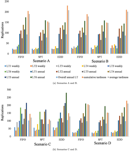
4.2.1. KPIs analysis

It is evident from Figure 6(a,b) how the benchmark Scenario A, without any disturbance, reports a lower number of observations compared to Scenario D and Scenario C with respect to lead times, highlighting an effect of these scenarios disturbances, rework time variability and rework likelihood, respectively. On the other hand, concerning tardiness KPIs, Scenario C seems to be the best one comparing the number of observations to all the others, even to the undisturbed scenario. Such result is obtained considering the confidence interval (Equation (3)(3) $CI=\bar{F}(L)\pm t_{n-1,\alpha /2}\frac{\sigma }{\sqrt{n}},$(3) ). For each sampled data, the respective confidence interval is calculated and divided for the sample mean, hence in Scenario C the standard deviation is higher compared to the basic scenario because of the disturbance (meaning wider confidence intervals) but the mean is higher as well, resulting in a tighter relative robustness. This finding indicates that this condition could be the most turbulent one and necessitates further investigation in the following analysis.

Considering, Scenario B, the number of observations for both lead times and tardiness KPIs is very similar to the basic operating conditions, stressing that assembly time variability does not have a great impact in robustness terms. To be robust against the different set of disturbances, the system has to be run for at least 280 observations with the set thresholds of 0.01 for the lead times KPIs and 0.02 for the tardiness ones. This observation number is $\gamma$ and was used in the ANOVA analyses to set the replications per policy and scenario. The indicators gathering more variability are the annual lead times as they demand more observations compared to the weekly ones across all the scenarios. Consequently, the KPIs reductions in the ANOVA analyses regarded the weekly lead times, focusing only on the annual ones for part types 1,2 and 3, overall annual LT and average tardiness.

In general, the increase in the assembly time has little impact on system tardiness but not on the different lead times consistently, while rework likelihood affects lead times robustness. The increase in the rework time variability affects on a medium scale lead times robustness compared to the assembly time increase and mostly tardiness indicators determining their higher values. The maximum number of observations to reach the threshold of 0.01 for the lead times and 0.02 for tardiness are 280 and is determined in the rework time variability scenario, this number is set as the basis to assume the system to be robust.

4.3. Full factorial design of experiments

Following the DoE analysis, an experimental design was devised to estimate the disturbances effects on the system. Considering 300 replications per policy averaged every 7 samples ($k$ set to 7), 120 points were obtained. The final dataset to perform the analysis, consequently, comprised 960 point per KPI, considering the 8 scenarios, enabling the disturbances main effects and disturbances interactions effects on the single KPI assessment. The experiments comprised the three disturbance factors on the same two levels of the experimental design, for a total of eight experiments, reported in Table 2.

The disturbances evaluated were listed along with the respective $p$-value and the percentage effect calculated according to Equation (4)(4) $\mathrm{\Delta }=\frac{KP{I}_{tot}}{\overline{KPI}}$(4) , where $KP{I}_{tot}$ is the total effect on the KPI and $\overline{KPI}$ is the mean value of the KPI across all scenarios.

(4) $\mathrm{\Delta }=\frac{KP{I}_{tot}}{\overline{KPI}}$(4)

The significance level for the $p$-value and the threshold to establish if an effect or an interaction was consistent were set to 0.05 and 5%, respectively, as shown in Table 4.

Table 4. 5% threshold values for the evaluated KPIs.

KPI	Mean across all scenarios	5% effect
Annual lead time part 1	227.20	11.36
Annual lead time part 2	194.40	9.72
Annual lead time part 3	229.10	11.46
Average lead time	211.40	10.57
Average tardiness	0.97	0.05

To examine the effects of different types of disturbances on the chosen KPIs, Table 5 summarises the effects on KPIs and the reported $p$-values.

Table 5. The effects of different types of disturbances on KPIs. When multiple disturbances are listed, their combination is considered.

Disturbance	KPI	LT1	LT2	LT3	Average	Average
		Annual	Annual	Annual	lead-time	tardiness
Assembly time	$p$-value	0.67	0.32	0.18	0.92	0.03
variability	Effect	0.11%	0.27%	−0.34%	0.02%	0.67%
Rework time	$p$-value	0%	0%	0%	0%	0%
variability	Effect	2.49%	2.51%	2.02%	2.39%	5.72%
Rework	$p$-value	0%	0%	0%	0%	0%
likelihood	Effect	16.79%	17.75%	14.12%	16.68%	38.31%
Assembly time variability	$p$-value	0.74	0.75	0.74	0.86	0.95
Rework likelihood	Effect	0.09%	−0.09%	−0.08%	−0.04%	−0.02%
Assembly time variability	$p$-value	0.98	0.95	0.95	1	0.98
Rework time variability	Effect	0.01%	0.02%	−0.02%	0%	0.01%
Rework time variability	$p$-value	0.04	0.73	0.15	0.09	0.01
Rework likelihood	Effect	0.54%	0.09%	0.36%	0.36%	0.75%
Assembly time variability	$p$-value	0.97	0.94	0.99	0.99	0.96
Rework time variability	Effect	−0.01%	0.02%	0%	0%	−0.02%
Rework likelihood

Rework likelihood resulted to have the main effect on the KPIs, rework time variability a little one while assembly time variability a negligible one. To improve robustness, the rework occurrence has to be tackled first to get the biggest advantage then the rework time variability could be object of intervention to foster performances even more.

4.4. ANOVA tests

4.4.1. ANOVA between scenarios

The proposed scenarios analysis is performed using the post-hoc results for each KPI, reporting the differences between the respective KPI means and the $p$-value as shown in Figure 7, where the first three part variants were reported as they are overwhelmingly the most frequently produced. The significance level ($\alpha$) was set to 0.05.

Figure 7. Differences between mean and $p$-value of KPIs as a comparison of scenarios.

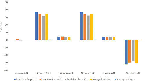
In Table 6, for each KPI and comparison the relative error was calculated to get a quantitative measurement of the detachment from the starting scenario using Equation (5)(5) $KP{I}_{re}=\frac{{\mathrm{\Delta }}_s}{{\mu }_{bs}}$(5) where ${\mathrm{\Delta }}_s$ is the difference between scenarios, and ${\mu }_{bs}$ is the mean of the KPI base scenario.

(5) $KP{I}_{re}=\frac{{\mathrm{\Delta }}_s}{{\mu }_{bs}}$(5)

Table 6. KPI relative error between scenarios.

Scenario	LT1	LT2	LT3	Average	Average
comparison	Annual	Annual	Annual	lead-time	tardiness
B - A	0.01%	0.4%	−0.27%	0.06%	0.85%
C - A	17.82%	19.84%	15.03%	18.01%	48.14%
D - A	2.14%	2.71%	1.81%	2.23%	6.34%

In Figure 7, it is noticeable that Scenario B and Scenario A are the same as the $p$-value is far higher than the significance set and the difference between the KPIs means is negligible. It can be stated that assembly time variability does not have any effect on the system. As a consequence, comparisons with Scenario B do not bring any information.

From the second row of Table 6, it is clear that Scenario C is the most turbulent as comparison against the basic operating conditions shows the highest difference concerning all the KPIs.

As far as Scenario D is concerned, from the third set of columns of Figure 7 and from Table 6 it can be observed that little changes occur compared to Scenario A for all the KPIs. Furthermore, rework time variability has little effect compared to the means of the KPIs themselves looking at Table 6 with a maximum of 2.71% and 6.34% concerning the lead times and the tardiness KPIs, respectively.

This analysis enabled a ranking of the disturbances based on their effect on the system. It could be noticed that Scenario C is the one causing the system to vary the most, therefore rework likelihood is the factor to focus on to improve robustness, system efficiency and enable the line to meet due dates promptly. From Table 6 is clear that it affects strongly all the KPIs compared to the starting scenario, especially tardiness with a 48% error.

On a second step rework time variability could be reduced as well, being related to rework occurrence and having some effect on system performances. A combined action would improve dramatically tardiness robustness and foster main lead times performances. Finally, assembly time variability resulted to have no significant effect on the KPIs.

4.4.2. ANOVA within each scenario

The presented policies analysis is performed using the post-hoc results for each KPI per scenario, reporting the differences between the respective KPI means per policy and the $p$-value. The significance level ($\alpha$) was set to 0.05. In the following sections the dispatching rules are compared, using two different types of tables, the first one reports the difference between the means for each KPI and the relevant $p$-value to give a general overview of the indicator’s behaviour. The second lists the relative errors per KPI and dispatching rule comparison with the FIFO rule, the benchmark one that is currently used. The formula used for the error is reported in Equation (6)(6) ${\epsilon }_r=\frac{{\mathrm{\Delta }}_{\mathrm{F}\mathrm{I}\mathrm{F}\mathrm{O}}}{{\mu }_{\mathrm{F}\mathrm{I}\mathrm{F}\mathrm{O}}}$(6) where ${\mathrm{\Delta }}_{\mathrm{F}\mathrm{I}\mathrm{F}\mathrm{O}}$ is the difference between the selected policy and FIFO, while ${\mu }_{\mathrm{F}\mathrm{I}\mathrm{F}\mathrm{O}}$ is the KPI mean according to FIFO policy. Only the results concerning the most turbulent condition, i.e. Scenario C, are reported.

(6) ${\epsilon }_r=\frac{{\mathrm{\Delta }}_{\mathrm{F}\mathrm{I}\mathrm{F}\mathrm{O}}}{{\mu }_{\mathrm{F}\mathrm{I}\mathrm{F}\mathrm{O}}}$(6)

If the error is higher than +5% the policy is assumed not to be able to cope with variability for the highlighted KPI. In Table 7 two examples are given per KPI type to give an estimate of the chosen threshold. If the error is negative, it means that the policy performs better than FIFO.

Table 7. Example of relative error per KPI type between the SPT and FIFO policies.

KPI	Difference	Mean	Relative error
LT2 Annual	10.38	208	4.99%
Average tardiness	0.04	0.79	4.86%

From Figure 8 and Table 8, it is noticeable that SPT performs worse than FIFO, going very close or exceeding the threshold for all the KPIs, except for average tardiness. On the other hand, EDD is better than FIFO for all the indicators except the annual lead-time of Part 3 (increase of 1.60%), returning good improvements of 2.28% and 3.01% for annual lead-time of Part 1 and annual lead-time for part 2 respectively. Similar results concerning the policies comparison were obtained for the remaining scenarios.

Figure 8. Comparison of release policy for Scenario A.

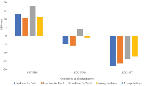
Table 8. KPI relative error of scenario C.

Policies	LT1	LT2	LT3	Average	Average
comparison	Annual	Annual	Annual	lead-time	tardiness
SPT - FIFO	5.26%	4.99%	7.96%	4.91%	2.44%
EDD - FIFO	2.28%	−3.01%	1.60%	−0.62%	1.11%

Comparing the dispatching rules across the different scenarios, it can be stated that SPT is not the policy to adopt as it usually returns worse results compared to FIFO for all the KPIs. On the other hand, EDD results to be always the best policy for the lead time for Part 1 and annual lead time for Part 2 and returns similar values in all the scenarios concerning average lead-time and average tardiness compared to FIFO as the $p$-values are high. Ultimately EDD performs worse than FIFO in each situation with a percentage ranging from 1.60% to almost 3%, not very high for annual lead-time of part 3, considering the share of part type 3 produced out of the total compared to part type 1, 2 and the fact that the average lead time gives good results as well showing a tendency to increase that has to be confirmed. In conclusion, EDD seems the policy to implement to foster the performances and improve the system robustness but a more detailed analysis is required to confirm the statement.

4.5. Financial implication estimate

Four main contributors were considered to estimate the financial implication of adopting the most robust dispatching policy (i.e. EDD): labour and electric power savings, material-holding savings, tardiness-related costs, cost to implement the new policy. Values were estimated on a yearly basis. Considering a labour cost of a machine operator of 9 GBP/hr and a cost of electric power of 0.13 GBP/kWh, the relevant savings were about GBP 49,816, when factoring-in relevant lead time and tardiness benefits. About GBP 950 were estimated to be saved in material-holding costs. Tardiness-related savings were estimated around GBP 50,000 multiplying the number of additional products delivered late by continuing to use FIFO and a penalty cost of GBP 1000 per part (considering not only customer charges but also overtime). Finally, although the implementation of EDD would not require changes on the shop-floor, 5 full days of an engineer were estimated for collecting the data, validate and verify the new policy (considering that the baseline DES model has been already implemented). Assuming a wage of 18 GBP/hr and 8 h a day of work, the cost is estimated to be GBP 720.

Combining the previously presented figures, it can be estimated that about GBP 100k can be saved in one year by switching from FIFO to the most robust policy (i.e. EDD).

5. Conclusion

A robustness evaluation framework has been developed and applied on a case study from the aerospace manufacturing sector. The application of the framework starts with a thorough definition of the manufacturing system, including the identification of the specific area of robustness that is to be evaluated. A simulation model, run methodically by experimental design is then developed and run for several replications. The outcome of the simulation model runs are then simultaneously analysed economically through a cost model and statistically through ANOVA tests.

The results, when the case study was applied to the framework, provided, with regard to operating conditions and dispatching rules, valuable practical insights. The results indicated, with regard to the impact of disturbances on the performance of the system, that assembly time variability has very little impact on performance, while rework likelihood having the most disruptive consequences on performance. On the dispatching rules side, the results demonstrated acceptable performance generated from adopting either FIFO or EDD rules, while the performance was significantly worse when an SPT rule was adopted.

Such illustrative case exemplified the usefulness of the framework to evaluate, analyze and recommend robustness improvements in manufacturing systems. The framework contributes to the scientific literature and, to the knowledge of the authors, is unique in being applicable to any type of disturbance described by any metrics using a multi-disciplinary collection of methods that formulate a detailed, pragmatic, methodical approach.

More in detail, existing, similar approaches do not address both strategic and operational disturbances or are limited to simplified representations of the manufacturing system to reduce the complexity of the mathematical problem (based on systems of differential equations) to enable the numerical solution and optimisation of the model. The proposed approach based on discrete event simulations solves this issue allowing the modeller to choose the preferred level of detail and capture the complexity of real manufacturing systems as much as desired. Although in the literature other simulation approaches can be found that avoid the mentioned numerical complexity with system dynamics, agent-based models or discrete event simulations, such methods do not present the detailed, methodical, multi-disciplinary process proposed in this work able to identify the deeper root causes of disruptions.

Further developments of the framework can be directed towards the implementation of the mentioned alternative simulation approaches (e.g. agent-based or system dynamics) that could be more suitable for peculiar manufacturing systems or robustness analyses. Furthermore, the financial implications could be further expanded and enriched with more comprehensive indicators that go beyond the computation of costs.

Disclosure statement

No potential conflict of interest was reported by the authors.

Data availability statement

Due to the nature of this research, participants of this study did not agree for their data to be shared publicly, so part of the supporting data is not available. Non-confidential data are available within the article.

References

- Adane, T. F., M. Floriana Bianchi, A. Archenti, and M. Nicolescu. 2019. “Application of System Dynamics for Analysis of Performance of Manufacturing Systems.” Journal of Manufacturing Systems 53 (September): 212–233. doi:10.1016/j.jmsy.2019.10.004.
- Adenso-Díaz, B., J. Mar-Ortiz, and S. Lozano. 2018. “Assessing Supply Chain Robustness to Links Failure.” International Journal of Production Research 56 (15): 5104–5117. doi:10.1080/00207543.2017.1419582.
- Alderson, D. L., and J. C. Doyle. 2010. “Contrasting Views of Complexity and Their Implications for Network-Centric Infrastructures.” IEEE Transactions on Systems, Man, and Cybernetics - Part A: Systems and Humans 40 (4): 839–852. doi:10.1109/TSMCA.2010.2048027.
- Barbé, K., W. Van Moer, and Y. Rolain. 2009. “Using ANOVA in a Microwave Round-Robin Comparison.” IEEE Transactions on Instrumentation and Measurement 58 (10): 3490–3498. doi:10.1109/TIM.2009.2018003.
- Blos, M. F., R. M. da Silva, and H. Ming Wee. 2018. “A Framework for Designing Supply Chain Disruptions Management Considering Productive Systems and Carrier Viewpoints.” International Journal of Production Research 56 (15): 5045–5061. doi:10.1080/00207543.2018.1442943.
- Borshchev, A., and A. Filippov. 2004. “From System Dynamics and Discrete Event to Practical Agent Based Modeling: Reasons, Techniques, Tools.” In The 22nd International Conference of the System Dynamics Society, Oxford.
- Chen, Y., H. Zhou, P. Huang, F. Chou, and S. Huang. 2022. “A Refined Order Release Method for Achieving Robustness of Non-Repetitive Dynamic Manufacturing System Performance.” Annals of Operations Research 311 (1): 65–79. doi:10.1007/s10479-019-03484-9.
- Chryssolouris, G. 2006. Manufacturing Systems: Theory and Practice. Second edi ed. New York: Springer.
- Colledani, M., D. Gyulai, L. Monostori, M. Urgo, J. Unglert, and F. Van Houten. 2016. “Design and Management of Reconfigurable Assembly Lines in the Automotive Industry.” CIRP Annals - Manufacturing Technology 65: 441–446. doi:10.1016/j.cirp.2016.04.123.
- Drira, A., H. Pierreval, and S. Hajri-Gabouj. 2007. “Facility Layout Problems : A Survey.” Annual Reviews in Control 31: 255–267. doi:10.1016/j.arcontrol.2007.04.001.
- Efthymiou, K., B. Shelbourne, M. Greenhough, and C. Turner. 2018. “Evaluating Manufacturing Systems Robustness : An Aerospace Case Study.” Procedia CIRP 72. 653–658. doi:10.1016/j.procir.2018.03.251, Elsevier B.V.
- Hopp, W. J., and M. L. Spearman. 2008. Factory Physics. 3rd ed. Long Grove, IL: Waveland Press.
- Kamalahmadi, M., M. Shekarian, and M. Mellat Parast. 2022. “The Impact of Flexibility and Redundancy on Improving Supply Chain Resilience to Disruptions.” International Journal of Production Research 60 (6): 1992–2020. doi:10.1080/00207543.2021.1883759.
- Kin, W., V. Chan, Y.J. Son, and C. M. Macal. 2010. “Agent-Based Simulation Tutorial - Simulation of Emergent Behavior and Differences Between Agent-Based Simulation and Discrete-Event Simulation.” In Proceedings of the 2010 Winter Simulation Conference, Baltimore, Maryland, USA, 135–150. IEEE.
- Klibi, W., A. Martel, and A. Guitouni. 2010. “The Design of Robust Value-Creating Supply Chain Networks: A Critical Review.” European Journal of Operational Research 203 (2): 283–293. doi:10.1016/j.ejor.2009.06.011.
- Kulturel-Konak, S. 2007. “Approaches to Uncertainties in Facility Layout Problems : Perspectives at the Beginning of the 21 St Century.” Journal of Intelligent Manufacturing 18: 273–284. doi:10.1007/s10845-007-0020-1.
- Law, A. M. 2015. Simulation Modeling and Analysis. Fifth edit ed. New York: McGraw-Hill Education.
- Maidstone, R. 2012. “Discrete Event Simulation, System Dynamics and Agent Based Simulation : Discussion and Comparison. System 1 (6): 1–6. https://scholar.google.co.uk/citations?view_op=view_citation&hl=en&user=DZsXj_8AAAAJ&citation_for_view=DZsXj_8AAAAJ:u5HHmVD_uO8C
- Meller, R. D., and K.Y. Gau. 1996. “The Facility Layout Problem: Recent and Emerging Trends and Perspectives.” Journal of Manufacturing Systems 15 (5): 351–366. doi:10.1016/0278-6125(96)84198-7.
- Meyer, M. 2016. “Redundancy Investments in Manufacturing Systems - The Role of Redundancies for Manufacturing System Robustness.” PhD diss., Jacobs University Bremen.
- Montgomery, D. C. 2017. Design and Analysis of Experiments. 9th ed. Hoboken, New Jersey: John Wiley & Sons, Inc.
- Pagone, E., K. Efthymiou, B. Mahoney, and K. Salonitis. 2019. “The Effect of Operational Policies on Production Systems Robustness: An Aerospace Case Study.” Procedia CIRP 81. 1337–1341. doi:10.1016/j.procir.2019.04.023, Elsevier B.V.
- Pinedo, M. L. 2016. Scheduling: Theory, Algorithms, and Systems. 5th ed. Berlin Heidelberg: Springer.
- Rakesh, N., R. C. Yadav, J. Sarkis, and J. C. James. 2000. “The Strategic Implications of Flexibility in Manufacturing Systems.” International Journal of Agile Management Systems 2 (3): 202–213. doi:10.1108/14654650010356112.
- Robinson, S. 2004. Simulation: The Practice of Model Development and Use. Hoboken: John Wiley & Sons.
- Saad, S. M., and N. N. Gindy. 1998. “Handling Internal and External Disturbances in Responsive Manufacturing Environment.” Production Planning & Control 9 (8): 760–770. doi:10.1080/095372898233533.
- Sabuncuoglu, I., and S. Goren. 2009. “Hedging Production Schedules Against Uncertainty in Manufacturing Environment with a Review of Robustness and Stability Research.” International Journal of Computer Integrated Manufacturing 22 (2): 138–157. doi:10.1080/09511920802209033.
- Sharda, B., and A. Banerjee. 2013. “Robust Manufacturing System Design Using Multi Objective Genetic Algorithms, Petri Nets and Bayesian Uncertainty Representation.” Journal of Manufacturing Systems 32 (2): 315–324. doi:10.1016/j.jmsy.2013.01.001.
- Siebers, P. O., C. M. Macal, J. Garnett, D. Buxton, and M. Pidd. 2010. “Discrete-Event Simulation is Dead, Long Live AgentBased Simulation!” Journal of Simulation 4 (3): 204–210. doi:10.1057/jos.2010.14.
- Stricker, N., and G. Lanza. 2014. “The Concept of Robustness in Production Systems and Its Correlation to Disturbances.” Procedia CIRP 19: 87–92. doi:10.1016/j.procir.2014.04.078.
- Stricker, N., A. Pfeiffer, E. Moser, B. Kádár, G. Lanza, and L. Monostori. 2015. “Supporting Multi-Level and Robust Production Planning and Execution.” CIRP Annals - Manufacturing Technology 64 (1): 415–418. doi:10.1016/j.cirp.2015.04.115.
- Sumari, S., R. Ibrahim, N. Hawaniah Zakaria, A. Hamijah, and A. Hamid. 2013. “Comparing Three Simulation Model Using Taxonomy : System Dynamic Simulation, Discrete Event Simulation and Agent Based Simulation.” International Journal of Management Excellence 1 (3): 4–9. doi:10.17722/ijme.v1i3.17.
- Telmoudi, A. J., L. Nabli, and M. Radhi. 2008. “Robust Control of a Manufacturing System : Flow-Quality Approach.” 2008 IEEE International Conference on Emerging Technologies and Factory Automation, Hamburg, Germany, 137–142.
- Thürer, M., M. Stevenson, C. Silva, M. J. Land, and L. D. Fredendall. 2012. “Workload Control and Order Release: A Lean Solution for Make-To-Order Companies.” Production and Operations Management 21 (5): 939–953. doi:10.1111/j.1937-5956.2011.01307.x.
- Tobias, B., A. Lange, and C. H. Glock. 2020. “Methods for Mitigating Disruptions in Complex Supply Chain Structures: A Systematic Literature Review.” International Journal of Production Research 58 (6): 1835–1856. doi:10.1080/00207543.2019.1687954.
- Tolio, T., M. Urgo, and J. Váncza. 2011. “Robust Production Control Against Propagation of Disruptions.” CIRP Annals - Manufacturing Technology 60 (1): 489–492. doi:10.1016/j.cirp.2011.03.047.
- Tsiamas, K., and S. Rahimifard. 2021. “A Simulation-Based Decision Support System to Improve the Resilience of the Food Supply Chain.” International Journal of Computer Integrated Manufacturing 34 (9): 996–1010. doi:10.1080/0951192X.2021.1946859.
- Yuchen, L., L. Zixiang, and F. Saldanha-da-Gama. 2021. “New Approaches for Rebalancing an Assembly Line with Disruptions.” International Journal of Computer Integrated Manufacturing 0 (0): 1–18.
- Zanchettin, A. M. 2022. “Robust Scheduling and Dispatching Rules for High-Mix Collaborative Manufacturing Systems.” Flexible Services and Manufacturing Journal 34 (2): 293–316. doi:10.1007/s10696-021-09406-x.
- Zhao, P., G. Shifu, and K. Yoshikawa. 2013. “An Orthogonal Experimental Study on Solid Fuel Production from Sewage Sludge by Employing Steam Explosion.” Applied Energy 112: 1213–1221. doi:10.1016/j.apenergy.2013.02.026.